Modelling dynamic portfolio risk
using risk drivers of elliptical processes
Rafael Schmidt
(Universität zu Köln)
Christian Schmieder
(Deutsche Bundesbank)
Discussion Paper
Series 2: Banking and Financial Studies
No 07/2007
Editorial Board:
Heinz
Herrmann
Thilo
Liebig
Karl-Heinz
Tödter
Deutsche Bundesbank, Wilhelm-Epstein-Strasse 14, 60431 Frankfurt am Main,
Postfach 10 06 02, 60006 Frankfurt am Main
Tel +49 69 9566-1
Telex within Germany 41227, telex from abroad 414431
Please address all orders in writing to: Deutsche Bundesbank,
Press and Public Relations Division, at the above address or via fax +49 69 9566-3077
Internet http://www.bundesbank.de
Reproduction permitted only if source is stated.
ISBN
978-
3–86558–
296
–
6
(Printversion)
ISBN
978-
3–86558–
297
–
3
(Internetversion)
Abstract
The situation of a limited availability of historical data is frequently encountered in portfolio risk estimation, especially in credit risk estimation. This makes it, for example, difficult to find temporal structures with statistical significance in the data on the single asset level. By contrast, there is often a broader availability of cross-sectional data, i.e., a large number of assets in the portfolio. This paper proposes a stochastic dynamic model which takes this situation into account. The modelling framework is based on multivariate elliptical processes which model portfolio risk via sub-portfolio specific volatility indices called portfolio risk drivers. The dynamics of the risk drivers are modelled by multiplicative error models (MEM) - as introduced by Engle (2002) - or by traditional ARMA models. The model is calibrated to Moody’s KMV Credit Monitor asset returns (also known as firm-value returns) given on a monthly basis for 756 listed European companies at 115 time points from 1996 to 2005. This database is used by financial institutions to assess the credit quality of firms. The proposed risk drivers capture the volatility structure of asset returns in different industry sectors. A characteristic temporal structure of the risk drivers, cyclical as well as a seasonal, is found across all industry sectors. In addition, each risk driver exhibits idiosyncratic developments. We also identify correlations between the risk drivers and selected macroeconomic variables. These findings may improve the estimation of risk measures such as the (portfolio) Value at Risk. The proposed methods are general and can be applied to any series of multivariate asset or equity returns in finance and insurance.
Key words: Portfolio risk modelling, Elliptical processes, Credit risk, multiplicative error model, volatility clustering, Moody’s KMV Credit Monitor database.
Non-technical summary
Over the past years, the availability of data for financial analysis in general and portfolio risk analysis in particular has substantially improved. This situation enables the use of more sophisticated methods for portfolio management and risk analysis and has attracted many scholars from the industry, academia, and banking supervision.
The present research project proposes a multidimensional stochastic dynamic model that identifies portfolio risk drivers via volatilities in two dimensions, over time and across in-dustry sectors. The identification and the need of modelling volatility dynamics in financial data goes (at least) back to the research by the Nobel laureate Robert Engle and has gained importance during the last two decades. The volatility is often referred to as the key driver of risk in a financial portfolio, and many performance measures or risk measures express the amount of risk via the volatility.
The model is applied to market-based credit risk data (monthly asset returns also known as firm-value returns) covering a limited period of time but comprising a large number of assets. The proposed method is particularly useful in the situation of a broad availability of cross-sectional data, i.e., a large number of assets in the portfolio. The data are obtained from the Moody’s KMV Credit Monitor database.
It is shown that the model is able to identify volatility patterns that remain otherwise hidden on the single-firm level. In this way, insights into the underlying factors which drive portfolio risk are possible. A characteristic temporal structure of the risk drivers, cyclical as well as a seasonal, is found across all industry sectors. In addition, each risk driver exhibits idiosyncratic developments. We also identify correlations between the risk drivers and selected macroeconomic variables. The findings may be used for the improvement and validation of Value at Risk estimates. The proposed methods are general and can be applied to any series of multivariate asset or equity returns in finance.
Nicht-technische Zusammenfassung
In den letzten Jahren hat sich die Verf¨ugbarkeit von Mikrodaten f¨ur finanzwirtschaftliche Untersuchungen, speziell im Bereich des Portfoliomanagements, deutlich verbessert. Im Zuge dessen ist das Interesse von Praktikern und Wissenschaftlern an komplexen stochasti-schen Methoden zur Anwendung im Bereich des Portfoliomanagements gewachsen. Nach wie vor besteht jedoch im Bereich der Kreditrisikoanalyse Nachholbedarf bei der Model-lierung und Validierung von Portfoliorisiken.
Die Autoren entwickeln ein mehrdimensionales stochastisches Modell, um dynamische Volatilit¨atsstrukturen zu identifizieren, welche das Portfoliorisiko treiben. Die Identifizierung und Modellierung von Volatilit¨aten in Finanzmarktzeitreihen spielt nicht zuletzt seit den bahnbrechenden Forschungsarbeiten des Nobelpreistr¨agers Robert Engle eine grundlegende Rolle f¨ur die Analyse von Portfoliorisiken. Die Volatilit¨at wird oft als der wichtigste Treiber des Portfoliorisikos bezeichnet und eine Vielzahl von bekannten Risiko- und Performance-maßen beschreibt das Risiko explizit anhand der Volatilit¨at.
Das vorgeschlagene stochastische Modell wird auf eine Zeitreihe von Kreditrisikodaten (monatliche Asset Renditen bzw. so genannte Firmwert Renditen) der Moody’s KMV
Credit Monitor Datenbank angewendet. Dieser Datensatz besitzt zwar eine beschr¨ankte
Historie, umfaßt jedoch eine große Anzahl von Firmen. Das stochastische Modell ist dabei besonders f¨ur diese Art von Datensituation geeignet.
Es zeigt sich, dass mit Hilfe des Modells Volatilit¨atsstrukturen erkannt werden k¨onnen, die ansonsten auf Einzelfirmenebene verborgen blieben. Hierbei sind besonders konjunkturbe-dingte Strukturen, unterj¨ahrige Saisonalit¨aten und branchenspezifische Charakteristiken von Interesse. Weiterhin werden Korrelationen zwischen den Risikotreibern und verschiede-nen makro¨okonomischen Indikatoren festgestellt. Die Ergebnisse k¨onnen verwendet wer-den, um die Modellierung und Sch¨atzung von Portfoliorisiken zu verbessern. Dar¨uber hin-aus eignet sich die Methode generell auch f¨ur andere finanzwirtschaftliche Fragestellungen, im Rahmen derer Portfoliorisiken modelliert und analysiert werden.
Contents
1 Introduction 1
2 Elliptical processes 3
2.1 Elliptical processes with single risk driver . . . 3
2.2 Risk-driver dynamics . . . 5
2.3 Generalized elliptical processes with multiple risk drivers . . . 6
2.4 Model Estimation . . . 7
2.4.1 Dispersion and location . . . 7
2.4.2 The risk driver . . . 8
2.5 Random number generation . . . 9
3 Analyzing and modelling portfolio credit risk 10 3.1 Data description . . . 10
3.2 Dynamics of the risk drivers . . . 12
3.2.1 Comparison between different industry sectors . . . 12
3.2.2 MEM versus ARMA model . . . 13
3.3 Risk drivers vis-`a-vis macroeconomic influences . . . 14
3.4 Dynamic VaR estimation in portfolios . . . 15
Modelling dynamic portfolio risk using risk drivers of
elliptical processes
11
Introduction
The motivation of this paper is based on a common situation in portfolio risk modelling, in particular credit risk modelling: time series data are sparse, while cross-sectional data are broadly available.2 The limitation of historical data may have various reasons, e.g., a limited collection or observation horizon, or a structural break due to a change in the collection methodology. Systematic data collection in financial institutions principally started during the last decade when sophisticated IT and database systems have been established. The database used in this study - Moody’s KMV Credit Monitor (in short: MKMV) database - is one of the most valuable sources for credit risk modelling and credit risk analysis. The database comprises credit risk relevant data of listed companies, such as credit exposures, expected default frequencies (EDFs), asset values or asset returns. Amongst others, this database has been used to calibrate the Basel II one-factor credit risk model, see Basel Committee on Banking Supervision (2006). MKMV asset returns are frequently used by financial institutions to estimate the asset correlations in structural credit risk models, cf. Lopez (2004) and Berndt et al. (2005). The data history of this database goes back to the beginning of the 1990s, but exhibits a structural break around the year 1995/1996. Thus for consistency reasons, the shorter time interval - from 1996 to 2005 - comprising only 115 monthly time observations for 756 listed European companies
is considered. We propose a high-dimensional stochastic model which takes this data
situation into account and is capable of capturing the temporal structure of portfolio risk via so-called risk drivers.
These risk drivers model the behavior of the sub-portfolio specific volatilities on an aggre-gated level. The identification and the need of modelling volatility dynamics in financial data goes (at least) back to the seminal work by Engle (1982) and Bollerslev (1986) and has gained importance during the last two decades.3 The volatility is often referred to as the key driver of risk in a financial portfolio, and many performance measures or risk measures such as the Sharpe ratio or the Value at Risk (VaR) in a Gaussian model -express the amount of risk via the volatility, cf. Jorion (2006). The general multivariate stochastic process, proposed in this paper, models the volatility using so-called risk drivers. These risk drivers enter the model as multiplicative factors and can be retrieved from the data. The stochastic process is termedelliptical processif it includes one single risk driver or generalized elliptical process if it includes multiple risk drivers, which are for example industry-specific. The risk drivers deliver information about the volatility in the portfolio which is otherwise not visible on a disaggregated single obligor level. This information is
1The first author gratefully acknowledges the hospitality and support of Deutsche Bundesbank. He would like to thank the Deutsche Forschungsgemeinschaft (DFG) for financial support. Further, the authors thank Thilo Liebig, Nick Bingham, R¨udiger Kiesel, Friedrich Schmid, Klaus D¨ullmann, Dirk Tasche, Christoph Memmel and the participants of the Second Bundesbank workshop on ’Research on financial stability’, in particular Peter Raupach, for inspiring and fruitful discussions. We are also grateful to the referees for valuable and helpful comments. Corresponding author: Rafael Schmidt, Universit¨at zu K¨oln, Seminar f¨ur Wirtschafts- und Sozialstatistik, Albertus-Magnus-Platz, D-50923 K¨oln, Germany, [email protected], Tel.: +49 221 470 2283, FAX: +49 221 470 5074.
2By cross-sectional we refer to the number of assets in the portfolio. 3For an overview see Alexander (2001) and references therein.
then incorporated into the portfolio risk estimation. Furthermore, risk managers may use the risk drivers as indicators of portfolio risk attributed to the volatility over time. An advantage of the proposed model is its fast random number generation. The model can be seen as a time-dynamic extension of the time-static model considered in Bingham et al. (2003).
The dynamics of the portfolio risk drivers are modelled by so-called multiplicative error models (MEM), as introduced by Engle (2002), and extended and applied by Chou (2005) and Engle and Gallo (2006). These dynamics capture the amount of volatility clustering inherent in the data via a GARCH-type structure. Alternative models such as nonlinear regression or trend models are also considered. A limiting argument even justifies the usage of traditional ARMA models for large portfolios.
Concerning the estimation of the multivariate dependence structure of the model, we sug-gest a simple correlation estimator which is based on ranks and is therefore robust. The estimator is called Blomqvist’s beta and is a measure of non-linear dependence that is solely determined by the copula of the multivariate distribution. A functional relationship between Blomqvist’s beta and the dispersion matrix of the generalized elliptical process shows that this measure of dependence is (asymptotically) consistent. In order to reduce the number of (correlation) parameters, we utilize the correlation structure of a one-factor model which is also the building block of the IRB portfolio model of Basel II, see Basel Committee on Banking Supervision (2006).
The set of competing multivariate volatility models can be divided into three categories. The first category consists of multivariate GARCH models and related types. Most promi-nent members are the DVEC(p,q) models (Bollerslev et al. 1988), the matrix-diagonal models (Ding 1994, Bollerslev et al. 1994), the BEKK models (Engle and Kroner 1995), the CCC model (Bollerslev 1990) or the PGARCH model (Alexander 1998). Without further restrictions, all these models estimate the volatility dynamics on the level of the univariate margins, however, for the (short horizon) risk data considered in this paper, no significant volatility structures can be found on this level. A common drawback of the unrestricted models is that the number of parameters to be estimated increases fast with increasing dimension and, thus, increases the forecast uncertainty - see also Gouri´eroux (1997) for an overview. We also mention EWMA models which are applied in practice, e.g., in the RiskMetrics proposal; see also Foster and Nelson (1996). In the univariate con-text, EWMA models correspond to IGARCH models. The second category are stochastic volatility models which model the volatility as a latent (unobserved) random source, see e.g. Tsay (2002) and references therein. They differ from our approach as we actually retrieve the risk drivers from the data. The third category of volatility models refers to the direct modelling of (univariate) portfolio returns as in McNeil and Frey (2000). This approach is useful in terms of dimensionality reduction and it certainly captures relevant volatility characteristics of the underlying assets. However, it ignores multivariate aspects which are, for example, necessary for portfolio allocation or the risk analysis of sub-portfolios. In the empirical study, the model is calibrated to Moody’s KMV Credit Monitor asset returns (also known as firm-value returns) for 756 listed European companies observed at 115 monthly time points from 1996 to 2005. A main finding is that the temporal structure of the volatility is statistically significant on the risk driver level only, whereas it is insignificant on the level of the single assets due to the limited data history. Furthermore, we observe temporal structures of the risk drivers which are similar across all industry sectors both in a seasonal and a cyclical context, with each sector’s risk driver also exhibiting idiosyncratic developments. We also find empirical correlations with selected macroeconomic variables.
These findings may be used to improve the quality of risk measurement via time-dynamic VaR models.
The paper is organized as follows. Section 2 introduces elliptical processes and the corre-sponding risk drivers. We start with a single risk driver in Section 2.1. Particular emphasis is placed on the interpretation of the risk driver and related examples of multivariate dis-tributions. Section 2.2 models the dynamics of the risk driver using a multiplicative error model (MEM) and provides possible extensions. Thereafter, Section 2.3 generalizes the models to multiple risk drivers and the subsequent sections elaborate its estimation and the corresponding random number generation. In Section 3 the model is applied to credit risk analysis. In particular, we calibrate the model to MKMV asset return data - described in Section 3.1 - and extract and model the risk drivers in Section 3.2. The following sections examine the empirical correlation of the risk drivers with selected macroeconomic variable and indicate their usage for portfolio VaR estimation. Section 4 concludes.
2
Elliptical processes
2.1 Elliptical processes with single risk driver
LetT be some countable index set representing time, i.e. setT ={. . . ,−1,0,1, . . .}.Ad -dimensional stochastic processX= (Xt)t∈T is calledelliptically contoured process(in short: elliptical process) if its marginsXt,for fixedt∈T, have the stochastic representation:
Xt=d m+RtAUt, (1) where mis a d-dimensional location vector and AA = Σ is a symmetric positive-definite
d×d dispersion matrix. The d-dimensional random vector Ut is uniformly distributed on the (d−1)-dimensional unit sphere Sd−1 := {x ∈ Rd :||x|| = 1},where || · || denotes the Euclidean norm, and Rt ≥0 is a one-dimensional random variable. The collection of random variables{Rt|t∈T} is stochastically independent of {Ut|t∈T}.Thus Xt,for fixedt∈T,possesses an elliptically contoured distribution, which is typically defined via a density function having a quadratic form as argument; for a review see Fang et al. (1990). The random variableRt,for fixedt,describes the radial part ofXtif Σ equals the identity matrix I and if the location vector m = 0. In that case, Ut denotes the angle vector, since a realization ofUtcorresponds to the angle ofXt(measured on the unit sphere). In particular, the following relationship holds
Rt=d ||(A)−1(Xt−m)|| and Ut=d
(A)−1(Xt−m)
||(A)−1(Xt−m)||. (2)
If E(R2t) < ∞, then the matrixctΣ corresponds to the variance-covariance matrix of Xt
with scaling factor ct =E(R2t)/d > 0. Thus, the variance-covariance matrix depends on the distribution of Rt which may be non-stationary.
Interpretation of Rt. Consider a portfolio comprising d assets, and let X describe the randomness of the d-dimensional asset returns. The process R = (Rt)t∈T is called the risk driver of X since it determines the degree of the overall volatility of X over time. More precisely,R is the random source which equally contributes to the volatility of each single-asset return and thus represents a driver of the overall volatility structure in the
example, volatility clustering - observed in many financial data - or seasonal volatility structures- found e.g. in high-frequency assets returns. In Section 3, we demonstrate that volatility clustering and seasonal volatilities are present in the KMV asset-return series. The main motivation of considering the risk driverRcomes from formula (2), which implies that - except for the estimation error of A and m- the distribution of R can directly be retrieved from the observations of X.
The collection of {Ut | t∈ T} is assumed to be mutually independent. This assumption appears to be reasonable in the present setting of few temporal observations but broad availability of cross-sectional data (thus, Ut is high dimensional). Besides, multivariate statistical tests for temporal correlation of the Ut will have low power in this setting.
Alternatively, Ut could be modelled as a random walk on the unit-sphere, cf. Bingham
(1972).
Examples. Elliptical processes are constructed by choosing different risk drivers R. In portfolio risk modelling, the tail behavior of the distribution of X is usually a key factor during the model-selection process. Heavy tails assign a higher probability to the (joint) occurrence of extreme events - such as extremely negative asset returns. In the following, we specify three distributions ofRtwhich yield either light tails, semi-heavy tails or heavy tails ofX.The temporal specification of R is left to the next section.
i) Heavy tails. Let Rt2/ν1 beF-distributed with ν1 and ν2 degrees of freedom, thus, Rt has density fR(x) = ν ν2/2 2 B(ν1/2, ν2/2) 2xν1−1 (ν2+x2)(ν1+ν2)/2, x >0, ν1, ν2>0
with beta-functionB.The tail decay offR(at infinity) is that of a power law, i.e.fR(x)∼
ax−b, b >0, asx→ ∞.The tail decay of the univariate margins of X
t possesses the same size, see Prop. 3.4 in Schmidt (2002). IfXtis ad-dimensional random vector, the particular choiceν1 =dyields a d-dimensionalStudent’st-distributionwithν2 degrees of freedom for
Xt.
ii) Semi-heavy tails. LetRt possess the Bessel-type density
fR(x) =c x ν−1 (1 +x2)ν/4−λ/2Kλ−ν/2(α 1 +x2), withc= α ν/221−d/2 Γ(ν/2)Kλ(α), x >0, λ∈R, ν, α >0,
whereKλ denotes the modified Bessel-function of the third kind with indexλ(see Magnus et al. (1966), pp. 65). The tail decay of fR (at infinity) is exponential of order one, i.e.
fR(x)∼axbexp(−cx), c >0,asx→ ∞,see Abramowitz and Stegun (1964), p.364, for the asymptotic expansion ofKλ for large arguments. The tail decay of the univariate margins ofXt is of the same size. IfXtis a d-dimensional random vector, the choiceν =d yields a
d-dimensionalgeneralized hyperbolic distributionforXt.We also refer to Barndorff-Nielsen and Blæsild (1981) who discuss semi-heavy tails of the univariate generalized hyperbolic distribution.
iii)Light tails. LetRt beχ-distributed with ν degrees of freedom, having density
fR(x) =
1
2(ν/2−1)Γ(ν/2)e
Note thatR2t isχ2-distributed withν degrees of freedom. The tail decay offR(at infinity) is exponential of order two, i.e. fR(x) ∼axbexp(−cx2), c >0, as x → ∞. The tail decay of the univariate margins of Xt possesses the same size. If Xt is a d-dimensional random vector, then the particular choiceν=d yields amultivariate normal distributionforXt. 2.2 Risk-driver dynamics
The risk driver R is a nonnegative valued stochastic process. Once the location m and
the dispersion Σ are estimated (cf. Section 2.4), R can be extracted using formula (2). The temporal structure ofR can be of any type, e.g., it may include deterministic trends, seasonal components, autoregressive components as well as volatility clustering. The fol-lowing model is useful if X exhibits volatility clustering; it takes the nonnegativity of R into account.
MEM dynamics. The risk driver R is decomposed into a conditionally deterministic scale factor - evolving according to a GARCH-type equation - and a positive innovation term. This type of model is known as multiplicative error model (MEM) and has been introduced in Engle (2002), see also Engle and Gallo (2006).
Let Ft = σ{Rs, s ≤ t} denote the information of the process R up to time t. Then Rt takes the form
Rt=μtεt withμt∈ Ft−1, εt⊥ Ft−1, andεt≥0. (3) The{εt}are independent and identically distributed (iid) with unit mean and varianceσ2, and the evolution ofμt depends on an unknown parameter vectorθ,i.e.μt=μt(θ).These conditions imply thatE(Rt| Ft−1) =μt and V ar(Rt| Ft−1) =σ2μ2t.The evolution of μt is modelled by some GARCH-type structure, which may also include asymmetric effects. For example, consider the GARCH(p, q)-type structure
μt=ω+ p i=1 αiRt−i+ q j=1 βjμt−j, p, q∈N, ω >0, αi, βj ≥0∀i, j. (4) The unconditional mean ofRtis then given byE(Rt) =ω/(1−αi−βj) for allt∈T. The choice of the distribution ofεt essentially determines the (un)conditional distribution of Xt. The example distributions stated in Section 2.1 yield a variety of possible distri-butions forεt.Initially, one should concentrate onRt being conditionally χ-distributed or
Rt2/dbeing conditionally F-distributed, which yield a d-dimensional normal or Student’s t-distribution forXt|Ft−1,respectively.
Boosting the dimension. Let Xt be d-dimensional and Rt(d) be the related risk driver, indexed by dimension d. Suppose that - conditional on Ft−1 - the risk driver R(td) is χ -distributed with d degrees of freedom. In case the dimensiond is very large, which means that the number of assets in the portfolio is very large, the following Fisher approximation eases the statistical estimation. Note that the MEM model is not yet implemented in statistical packages. The Fisher approximation yields
R(td)−
d−1/2−→d Rt(∞) ∼N(0,1/2) asd→ ∞.
Thus for large portfolios, the risk driver can be approximated by a non-centered normal distribution, whose negative values occur with negligible likelihood. A rule of thumb for a
sufficiently good approximation is d ≥ 40, see e.g. Severo and Zelen (1960) for empirical results and alternative approximations. An advantage of the approximation is that the innovations{εt} - in the MEM model centered byd−1/2 - need not to be nonnegative anymore. Hence, traditional ARMA models represent a possible alternative for the risk driver dynamics. Our empirical study shows that for large portfolios the MEM model and the ARMA model yield similar results.
If - conditional on Ft−1 - the risk driver (R(td))2/d is F-distributed with ν1 = d and ν2 degrees of freedom, then the following approximation holds
R√(td) 2
d
R˜(d)
t for larged,
where ˜R(td) has a noncentral Student’s t-distribution withν2 degrees of freedom and cen-trality parameterd−1/2.
2.3 Generalized elliptical processes with multiple risk drivers
The elliptical process defined so far is driven by a single risk driver. This process is applicable if thedasset returns are equally distributed - except for a different dispersion or location. However, if we consider a portfolio consisting of assets which belong to different industries or geographical regions, the assumption of equally distributed returns may be violated. We therefore define generalized elliptical processes, which allow for different risk drivers in different sub-portfolios and which include elliptical processes as a special case. Ad-dimensional stochastic processX= (Xt)t∈T is calledgeneralized elliptical process(with
ksectors) if its margins Xt,for fixedt∈T, have the following stochastic representation:
Xt=d m+ (R∗t,1Vt,1, R∗t,2Vt,2, . . . , R∗t,kVt,k) (5) with random vectorsVt,1 = (Vt,1, . . . , Vt,j1),Vt,2 = (Vt,j1+1, . . . , Vt,j2), . . . ,Vt,k= (Vt,jk−1+1,
. . . , Vt,d) such that Vt = (Vt,1, . . . ,Vt,k) = AUt and Ut is uniformly distributed on the (d−1)-dimensional unit sphere Sd−1. In formula (5), the vector of vectors is under-stood as a d-dimensional vector, which is a slight abuse of notation. The collection of
{Vt | t ∈ T} is assumed to be mutually independent. Moreover, the random variables
{R∗t,i |t ∈ T, i = 1, . . . , k} are stochastically independent of {Vt |t ∈ T}. The temporal and contemporaneous (across the sectorsi) dependence structure between the risk drivers
Rt,i∗ can be of any type. For example, the contemporeneous dependence structure may take the form
R∗t,i =fi(Rt), i= 1, . . . , k, (6) for some nonnegative increasing functionsfi and random variableRt; similar to the model by Daul et al. (2003). The interpretation of this model is that the risk driversR∗t,i are com-pletely correlated across the sectors, but there impact per sector is of different magnitude. This approach allows, e.g., to model a different tail distribution per sectors.
Given the sector i∈ {1, . . . , k},the following holds:
||(Bi)−1(Xt,i−mi)||=d ||R∗t,iVt,i||=d Rt,i, i= 1, . . . , k, (7) where BiBi = Σ(ii), Σ(ii) is the i-th partition-matrix of Σ, Xt,i = (Xt,ji−1+1, . . . , Xt,ji), and mi is the i-th partition-vector of m, corresponding to sector i. Further, Rt,i denotes
the radial variable or risk driver of the elliptical process Xt,i = (Xt,ji−1+1, . . . , Xt,ji).The relationship betweenRt,i and R∗t,i is
Rt,i=d Bt,i·Rt,i∗ , (8) where (Bt,21, . . . , B2t,k) ∼ Dk(j1/2,(j2 −j1)/2, . . . ,(jk−jk−1)/2) is Dirichlet distributed. Moreover, the collection{Bt,i}is stochastically independent of{R∗t,i}.The proof of formula (8) is analogue to the proof of Theorem 2.6 in Fang et al. (1990), p. 33; see also Chapter 1.4 in this reference.
2.4 Model Estimation
A two-stage estimation is utilized in order to estimate the distribution of X. First, we estimate the (time invariant) parametersmand Σ,and, second, we identify the distribution of the risk driversRt,i, i= 1, . . . , k.
2.4.1 Dispersion and location
In the situation of only few temporal observations but a broad availability of cross-sectional data, the large number of parameters in the dispersion matrix Σ would yield an over-specification of the model. One way to reduce the number of parameters is the consideration of factor models, which is frequently done in portfolio risk modelling, see e.g. the internal model proposed by the Basel Committee on Banking Supervision (2006). Let us first assume that X is an elliptical process with single risk driver R, representing the asset returns of a portfolio withk sectors (or sub-portfolios). A simple one-factor model is
(Xt,j−mj)/Σjj =d ωjZt+
1−ω2jεt,j for j= 1, . . . , d, t∈T, (9) where theωj areequalifXj belongs to the same sector. Here, we assume that the (d+ 1)-dimensional vector (Zt, εt,1, . . . , εt,d)has unit dispersionI,zero location, and belongs to the same family of elliptical distributions as Xt. The correlation entries of the corresponding dispersion matrix Σ take the form ρij = Σij/ΣiiΣjj = ωiωj if i = j. Note that this parameter reduction implies that the ρij coincide if i and j, respectively, belong to the same sector. Estimators of ρij - within this factor model - have been discussed in the literature, see e.g. Gordy (2000) and references therein. They are either based on ML-procedures or Pearson’s sample covariance. However, ifXis a generalized elliptical process with multiple risk drivers, these estimators may not be suitable as they are not necessarily (asymptotically) consistent. An example is given in table 1, where we estimate ρij of a generalized elliptical process by Pearson’s sample correlation.
Because of these findings, we provide an alternative estimator for the correlation param-eters, which is (asymptotically) consistent. First, we make the following observation: Let
Xt,iandXt,j be thei-th andj-th margin ofXtbelonging to a generalized elliptical process
X.IfP (Xt,j = ˜xt,j) = 0 for all j= 1, . . . , d, then
P (Xt,i<x˜t,i, Xt,j <x˜t,j) = P R∗t,kiVt,i<0, R∗t,kjVt,j <0 (10) = P (Vt,i<0, Vt,j <0) = P (Zt,i <0, Zt,j <0),
where ˜xt,i=mi is the median of Xt,i and Zt∼Nd(0,Σ).For the last equality, we utilized the observations of example iii) in Section 2.1. Thus, the orthant probabilities of (Xt,i, Xt,j) are invariant with respect to the risk driver R. However, there exists a well-known rela-tionship between the orthant probabilities of a d-dimensional normal distribution and the correlation parametersρij = Σij/ΣiiΣjj:
4P(Xt,i <x˜t,i, Xt,j <x˜t,j)−1 = 4P (Zt,i <0, Zt,j <0)−1 = 2 arcsin(ρij)/π. (11) The left-hand side of equation (11) corresponds to the population version of Blomqvist’s beta - denoted byβij - which is a rank-based dependence measure introduced in Blomqvist (1950). The sample version of Blomqvist’s βij between the i-th and j-th margin of X is defined by ˆ βij = 2 n n t=1 1 {Uˆt,i(n)≤1/2,Uˆt,j(n)≤1/2}+1{Uˆt,i(n)>1/2,Uˆt,j(n)>1/2} −1,
where ˆUt,i(n)= n1(rank of Xt,i in X1,i, . . . , Xn,i); for related results on asymptotic normality and efficiency we refer to Schmid and Schmidt (2006). Thus for a generalized elliptical process, an asymptotically consistent and robust estimator ofρij is given by
ˆ
ρij = sin(πβˆij/2). (12)
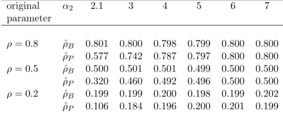
The correlation parameters ofXwithin one sector and between two sectors are then derived as the average of the ˆρij which belong to the one sector and the two sectors, respectively. The positive definiteness of the resulting dispersion matrix - if it is not already given - can be obtained by using techniques proposed e.g. in Rousseeuw and Molenberghs (1993). Table 1 illustrates the magnitude of the bias ifρij is estimated using Pearson’s sample cor-relation. Though the bias is usually small it may become large if one marginal distribution is light tailed while another marginal distribution is heavy tailed.
The location vectormand the dispersion parameters Σjj, respectively, are e.g. estimated by the sample median and the (trimmed) sample variance; these estimators are consistent if the risk drivers are ergodic. Further parameter restrictions could be imposed on the (volatility) parameters Σjj.We set ˆΣij := ˆρij
ˆ
ΣiiΣˆjj ifi=j.
Approximate realizations of the risk drivers Rt,i are now obtained using formula (7). In particular,
ˆ
Rt,i:=||( ˆBi)−1
Xt,i−mˆi||, i= 1, . . . , k (13) where ˆBiBˆi= ˆΣ(ii).Suitable stochastic processes may now be identified for the time series
ˆ
Ri = ( ˆRt,i)t∈T.The estimation of an MEM model - given in Section 2.2 - is discussed next.
2.4.2 The risk driver
Let (Rt)t=1,...,ndenote the (approximate) observations of the risk driverR.In order to ease the presentation, we assume that R is the (single) risk driver of ad-dimensional elliptical
process. Let R evolve according to the MEM model given in formula (3). Suppose that
Rt|Ft−1 is χ-distributed with ν > 0 degrees of freedom yielding a d-dimensional normal
distribution for Xt|Ft−1 if ν = d. This choice is closely related to the error distribution
Table 1: Estimated correlation parameter ρ using Blomqvist’s ˆβ as in formula (12) - this estimator is denoted by ˆρB- or using Pearson’s sample correlation ˆρP.The underlying data have been generated from a bivariate generalized elliptical process - as given in formula (5) - with Xt,1 (andXt,2) being t-distributed random variables with α1 = 7 (and α2) degrees of freedom - which are independently drawn across time. The sample length is one million.
original α2 2.1 3 4 5 6 7 parameter ρ= 0.8 ρˆB 0.801 0.800 0.798 0.799 0.800 0.800 ˆ ρP 0.577 0.742 0.787 0.797 0.800 0.800 ρ= 0.5 ρˆB 0.500 0.501 0.501 0.499 0.500 0.500 ˆ ρP 0.320 0.460 0.492 0.496 0.500 0.500 ρ= 0.2 ρˆB 0.199 0.199 0.200 0.198 0.199 0.202 ˆ ρP 0.106 0.184 0.196 0.200 0.201 0.199
Note that Pearson’s correlationρis not well defined forα2≤2.
the error term, i.e. εt|Ft−1 ∼ Gamma(φ, φ), φ > 0. Note that the χ2-distribution - not theχ-distribution - is a special case of theGamma-distribution. Since our primary focus is rather on multivariate modelling, we adopt the χ-distribution for R which yields the multivariate normal distribution as a special case for X.More precisely, we assume that
c·εt| Ft−1 ∼χ(ν) =⇒ Rt| Ft−1 ∼(μt/c)·χ(ν), ν >0, (14) with c=√2Γ{(ν+ 1)/2}/Γ(ν/2).The scaling of εt by c ensures the identifiability of the model, i.e.E(εt|Ft−1) = 1. Note that for ν =d, Xt|Ft−1 possesses a multivariate normal distributions.
Under assumption (14), the contribution of a generic observation rt to the log-likelihood functiont is t= lnLt= 1−ν 2 ln 2−ln Γ ν 2 +νlnc−νlnμt+ (ν−1) lnrt− c μt 2r2 t 2 . Using this formula, one can calculate the contribution of rt to the score, the Hessian, and the first order conditions for the ML estimation of the MEM model.
In case the densities ofRt|Ft−1, t∈T, belong to the same exponential family
f(rt|Ft−1) = exp[ν{rtϑt−b(ϑt)}+d(rt, ν)],
the MEM model is a member of the family of Generalized Linear Autoregressive Moving Average (GLARMA) models as pointed by Cipollini et al. (2006); for more background on this family we refer to Benjamin et al. (2003) and references therein.
2.5 Random number generation
An advantage of generalized elliptical processes is their feasible simulation even in very high dimensions. This is because the simulation reduces more or less to the simulation of
the risk drivers and, thus, eases the curse of dimensionality. A simulation algorithm for generating paths of generalized elliptical processes is given next. Assume that the location vector mand the dispersion matrix Σ are known (or estimated, respectively). Note that the generation of sample paths from a single risk driver is a univariate problem. In this case, the distribution of the risk drivers R and R∗ in formula (8) coincides. The case of multiple risk drivers is more involved. For the time being assume that the dynamics of the risk drivers Ri and R∗i - as specified in (8) - are given as well as the related generation algorithms.
Algorithm of generating pseudo-random paths of generalized elliptical pro-cesses:
Step 1 Calculate Σ =AA, e.g., using Cholesky decomposition. Step 2 Sample a path of lengthnfrom (R∗t,1, . . . , R∗t,k).
Step 3 Sample d times n independent random numbers Zt,1, . . . , Zt,d, t = 1, . . . , n,from a univariate standard-normal distribution N(0,1). Step 4 Set Zt= (Zt,1, . . . , Zt,d) for t= 1, . . . , n.
Step 5 Set Ut=||Zt||−1·Zt fort= 1, . . . , n. Step 6 Set
Vt= (Vt,1, . . . ,Vt,k) =AUt
with Vt,1 = (Vt,1, . . . , Vt,j1), Vt,2 = (Vt,j1+1, . . . , Vt,j2), . . . , Vt,k = (Vt,jk−1+1, . . . , Vt,d).The partition corresponds to the sector partition. Step 7 ReturnXt=m+ (R∗t,1Vt,1, R∗t,2Vt,2, . . . , R∗t,kVt,k).
In the case of multiple risk drivers Rt,i,one needs to derive the (conditional) distribution ofR∗t,i.First, the distribution of (Rt,1, . . . , Rt,k) is identified using the estimation procedure elaborated in Section 2.4.1. Thus, given the informationFt−1,the distributions ofRt,i and
Bt,i in formula (8) are known. Taking the logarithm on both sides of formula (8) shows that the extraction of the distribution ofRt,i∗ is a deconvolution problem which is typically considered in signal and image processing. The distribution ofRt,i∗ may either be retrieved by explicit or numerical deconvolution, see Haykin (2000) for more background and related references.
3
Analyzing and modelling portfolio credit risk
In the present section, the above theoretical framework of generalized elliptical processes is applied to the risk analysis and risk modelling of a credit portfolio.
3.1 Data description
The empirical analysis is based on data from Moody’s KMV Credit Monitor (in short: MKMV) and covers the period from February 1996 to August 2005. MKMV utilizes a structural Merton-type credit risk model (Merton 1974) that has been refined using em-pirical evidence and is commonly used among practitioners in order to assess a firm’s creditworthiness. MKMV provides, for example, so-called expected default frequencies(in short: EDFs) which refer to the firms’ probability of default and, thus, to its
creditwor-thiness.4 The EDF is calculated as the likelihood that the firm’s asset value falls below a given default threshold. The original Merton model (Merton 1974) treats the firm’s equity as a call option on the firms asset value. These asset values form the basis of the forthcom-ing analysis. We start with an analysis of the time dynamics of the related risk drivers. Afterwards, these risk-driver dynamics are used for credit Value at Risk (VaR) estimation. The data set comprises of credit risk data of 756 European non-financial firms with publicly traded equity, amongst others, it comprises asset values, asset returns, EDFs and exposures (the firms’ total liabilities).5 From February 1996 to August 2005, there are 115 monthly observations available. We have particularly chosen this time horizon since the MKMV methodology was adjusted by the end of 1995. Thus, a consideration of asset values before and after this structural break may cause inconsistencies. The chosen time period covers up-and downturns in the financial markets e.g. induced by the Asian crises (around 1997/98) and the September 11, 2001 event. The firms are assigned individually to six industry sectors as defined by MKMV. These industry sectors are Basic and Construction Industry (BasCon), Consumer Cyclical (ConCy), Consumer Non-Cyclical (ConNC), Capital goods (Cap), Energy and Utilities (EnU) and Telecommunication and Media (Tel). Descriptive statistics of the database are shown in table 2.6
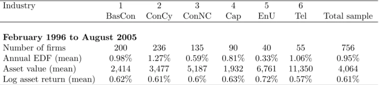
Table 2: Descriptive statistics of the data set
Asset values are measured in million euros and corresponding log returns are calculated on a monthly basis. The total sample values are averaged over all firms in the sample. BasCon refers to Basic and Construction Industry, ConCy to Consumer Cyclical, ConNC to Consumer Non-Cyclical, Cap to Capital goods, EnU to Energy and Utilities and Tel to Telecommunication and Media.
Industry 1 2 3 4 5 6
BasCon ConCy ConNC Cap EnU Tel Total sample
February 1996 to August 2005
Number of firms 200 236 135 90 40 55 756
Annual EDF (mean) 0.98% 1.27% 0.59% 0.81% 0.33% 1.06% 0.95%
Asset value (mean) 2,414 3,477 5,187 1,932 6,761 11,350 4,064
Log asset return (mean) 0.62% 0.61% 0.6% 0.63% 0.72% 0.57% 0.61%
The largest industry sectors are ConCy and BasCon comprising 31% and 26% of the total number of firms in the portfolio. The second largest sectors are ConNC and Cap with 18% and 12% of the total portfolio. The third group consists of Tel and EnU with a portfolio size of 7% and 4%. It is shown below that the sector size has an impact on the level of the risk driver. The mean EDFs of the sectors range from 0.33% in the EnU sector to 1.27% in the ConCy sector. The largest firms in the sample are contained in Tel, which exhibit on average a five times higher asset value than Cap firms (11.4bn Euros vis-a-vis 1.9bn Euros). The average asset returns over the time horizon February 1996 to August 2005
-4For further information about the MKMV methodology see, for example, Crouhy et al. (2000) and references therein.
5We assume that the distribution of the firms’ total liabilities represents the exposure distribution of a hypothetic credit portfolio.
6The raw MKMV database has been modified in two aspects. First, all asset returns have been trans-formed into Euro currency; Before 1998, Deutsche Mark (DEM) has been used as a reference currency. Second, only time series without missing or erroneous asset values, EDFs and exposures are considered.
are around 0.62% in all industry sectors.
3.2 Dynamics of the risk drivers
We start with analyzing the time dynamics of the risk drivers.
3.2.1 Comparison between different industry sectors
Figure 1 compares the time evolution of the risk driversRt,i by utilizing formula (13) -for various pairs of industry sectors, namely the risk driver -for the Basic and Construction sector (BasCon) together with the risk driver from a sector with
i) large sector size (industry sector 2: ConCy), ii) middle sector size (industry sector 4: Cap), and iii) small sector size (industry sector 6: Tel).
1996 1998 2000 2002 2004
51
5
Risk driver R of industry 1 (BasCon) Risk driver R of industry 2 (ConCy)
1996 1998 2000 2002 2004
51
5
Risk driver R of industry 1 (BasCon) Risk driver R of industry 4 (Cap)
1996 1998 2000 2002 2004
51
5
Risk driver R of industry 1 (BasCon) Risk driver R of industry 6 (Tel)
Figure 1: Risk-driver dynamics of MKMV asset returns for industries 1, 2, 4, and 6. We observe a positive correlation between the sector size and the level of the risk driver, for example, the risk driver exhibits a higher nominal level for the BasCon sector compared to the Tel sector. This outcome is expected, as it implies that the total risk in a sub-portfolio increases with the number of firms. Second, we find that the risk drivers tend to exhibit peaks at 12-month time intervals, particularly for the BasCon and for the Cap sector. This can be explained as follows. The MKMV asset values are based on the market value of the firms’ equity and the book-value of the firms’ liabilities. In most cases, MKMV updates the balance sheet data of European firms once every 12 months. For example, for the BasCon this usually happens in April, May or June. Thus, the volatility of the asset values tends to increase around this time and is causally related to the development
of the sector-specific risk drivers in these months. The update of the firms’ liabilities is particularly important for asset-rich firms, such as firms in the BasCon sector, and for firms which exhibit substantial balance sheet reorganization.
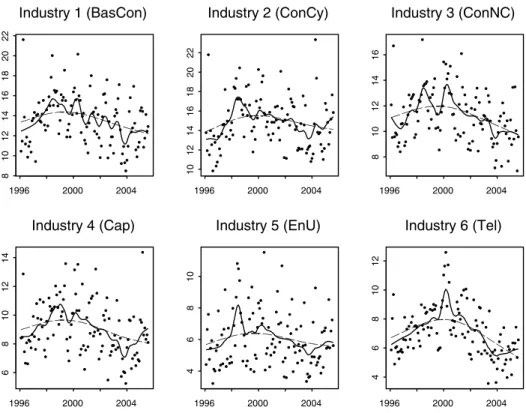
Moreover, all risk drivers show a characteristic long-term pattern or cyclical trend, which becomes apparent in figure 2, where we use a different scaling. The level of the risk drivers increases until 2000, followed by a decrease of the same magnitude until the end of the observation period. This pattern is particularly pronounced for the Tel sector; by contrast, there is a less characteristic 12-month seasonality. The reason is that most firms in the Tel sector have undergone a dynamic development and a substantial increase of their equity basis during the observation period, and the volatility of their equity value has already been on a high level. This implies that the balance sheet updates had a lower impact on the risk driver in the Tel sector. By contrast, the EnU sector shows a modest overall cyclical behavior in the risk driver.
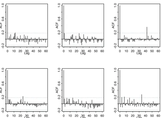
In summary: The risk drivers of all industries show temporal dependencies which are also confirmed by the autocorrelation functions given in figure 3. We point out that a main motivation of considering risk drivers was the finding of those autocorrelations on the aggregate risk-driver level. By contrast, no significant autocorrelations of the asset returns and the squared asset return were found on the single (disaggregated) firm level, cf. figure 4.
3.2.2 MEM versus ARMA model
Following our exposition in Section 2.2, we estimate an MEM and an ARMA model for the risk driver in each industry sector and compare both. The ARMA model is motivated by the large number of firms in each sector and the findings of Section 2.2. We identify the simplest MEM model by considering a GARCH(1,0)-type structure in equation (4), and compare it to the corresponding ARMA model, namely the AR(1) model. The innovation terms are assumed to be normally distributed, which is justified below. The respective models are denoted by MEM(lag1) and AR(lag1). Additionally we fit two more autoregressive structures: in the first case we regress on lag 12 (in short: AR(lag12)) and in the second case we regress on lags 1 and 12 (in short: AR(lag1; lag12)). The motivation for the latter two models is the observed 12-month seasonality of the risk drivers, described in the previous section. The estimated parameters (except the intercept) are provided in table 3. The residuals of the estimated MEM(lag1) and AR(lag1) model are shown in figures 5 and 6.
From table 3 and figures 5 and 6 we conclude:
i) The estimated parameters (or loadings) of the MEM(lag1) and the AR(lag1) model are close to each other. Moreover, the QQ-plots of the corresponding residuals possess a very similar structure. In particular they show that the normal innovations are a reasonable choice for the MEM and the AR model in this setting. The forecast quality of the AR(lag1) model is illustrated in figure 7. We remark that the QQ-plots of the (original) risk-driver realizations are highly skewed, which again justifies the usage of MEM or AR models.
ii) One reason that the results of the MEM and the AR model are close to each other is the large number of firms in each industry sector and the limiting argument given in Section 2.2.
iii) The industry sectors 1 and 4 show a large AR-parameter (or loading) at lag 12 which is in line with the findings in figure 3. See also the related discussion in Section 3.2.1.
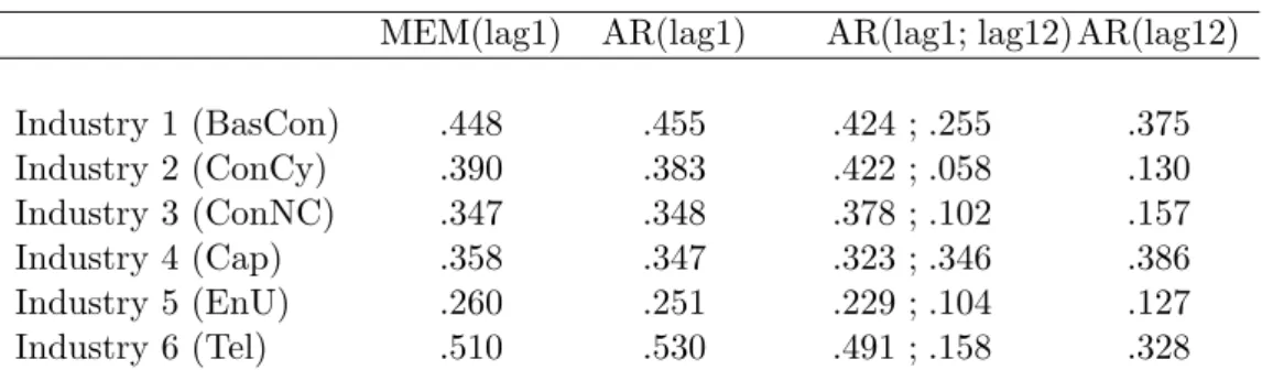
Table 3: Parameter estimates (except the intercept) of the risk driver following an MEM or ARMA model per industry sector.
MEM(lag1) AR(lag1) AR(lag1; lag12) AR(lag12)
Industry 1 (BasCon) .448 .455 .424 ; .255 .375 Industry 2 (ConCy) .390 .383 .422 ; .058 .130 Industry 3 (ConNC) .347 .348 .378 ; .102 .157 Industry 4 (Cap) .358 .347 .323 ; .346 .386 Industry 5 (EnU) .260 .251 .229 ; .104 .127 Industry 6 (Tel) .510 .530 .491 ; .158 .328
All parameters are statistically significantly different from zero at a confidence level of 1%.
3.3 Risk drivers vis-`a-vis macroeconomic influences
We analyze possible correlations between the sector-specific risk drivers and selected macroe-conomic variables.7 German macroeconomic variables are utilized as the majority of firms in the data sample are based in Germany. We consider the following six macroeconomic variables: The seasonally adjusted unemployment rate,8the gross domestic product (GDP), an index for the industry production (Ind Product), the money-market rates for three-month funds (InterestRate), the development of order bookings in the industry (Order-Bookings) and the inflation rate (CPI).9 The (sample) correlations between the macroe-conomic variables and the risk drivers are presented in table 4. The three macroemacroe-conomic variables which exhibit the highest correlation with the risk drivers are the interest rate, the unemployment rate and the GDP. For those variables, the highest correlation is found for the Tel sector, the ConNC sector and the Cap sector. The results for the Tel sector (industry 6) confirm the fact that the business of Tel firms is affected by the cyclical be-havior of the economy. This effect is particularly revealed by the strong correlation with the interest rate and the unemployment rate. The ConNC sector (industry 3) is known to be sensitive towards changes of consumer price levels, which is reflected in the correlation with both the CPI and the interest rate. Also the correlation with the unemployment rate - which has an impact on the consumption behavior - is in line with our expectations. The fact that the interest rate exhibits the highest correlation with all risk drivers demon-strates the importance of this economic variable for monetary policy. For the unemploy-ment rate, the correlations are negative, which implies that a higher unemployunemploy-ment rate comes along with a lower level of the risk driver. The GDP shows a moderate correlation with the risk drivers ranging from 7% to 10%. Figures 8 and 9 illustrate the co-movement between the risk drivers and the interest rate and unemployment rate, respectively. In sum, the previous results show that the cyclical behavior of the economy has an impact on the (temporal) development of the risk drivers in most industries.
7Statistical influences of macroeconomic variables on credit risk have been investigated by some authors, see e.g. Allen and Saunders (2003) and references therein.
8The unemployment rate and the GDP are used with a lag of six months in order to incorporate the time lag where the cyclical effects become evident.
9Robustness studies show that the corresponding macroeconomic variables of France and the UK produce similar results.
Table 4: Sample correlation of selected macroeconomic variables with the industry-specific risk drivers. ’Unemploy’ refers to the unemployment rate, ’GDP’ to the gross domes-tic product, ’Ind Product’ to the industry production, ’InterestRate’ to the three-month money market rate, ’OrderBookings’ to the index of order bookings in the industry, and ’CPI’ to the development of the price level.
Risk driver Unemploy GDP Ind Product InterestRate OrderBookings CPI
Industry1 (BasCon) -16.7% 8.8% 1.0% 21.9% 1.3% -4.5% Industry2 (ConCy) -22.3% 7.6% 15.5% 17.7% -9.6% 0.6% Industry3 (ConNC) -23.9% 10.4% 0.6% 34.7% -12.7% 12.3% Industry4 (Cap) -14.5% 9.7% 7.4% 24.0% -12.0% 0.8% Industry5 (EnU) -13.3% 7.4% 8.3% 17.2% -12.8% 5.0% Industry6 (Tel) -47.1% 7.0% -0.4% 51.7% 1.5% 4.1%
The correlations for Unemploy, GDP, and InterestRate are all significantly different from zero at 1% level.
3.4 Dynamic VaR estimation in portfolios
The Value at Risk (VaR) of a portfolio - comprising d assets - is the current standard risk measure in practice and in the regulatory framework (Basel Committee on Banking Supervision 2006). In this framework, the dynamic VaR of a credit portfolio is calculated from the portfolio loss distributionL given by
Lt= d
j=1
wt,jψt,j1{Xt,j≤Kj}, t∈T, (15)
where wt,j denotes the relative exposure of obligor j at time t ∈ T which is defined as the ratio of the book value of liabilities of obligor j with respect to the aggregated book value of liabilities in the portfolio; obtained from the MKMV database. A justification for the latter definition is given in Duellmann et al. (2006), p.15. Further, ψt,j refers to the loss severity at default, which we assume to be constant at 45%, Kj is the obligor-specific default threshold, andX= (Xt)t∈T denotes the process of asset returns. The loss severity of 45% corresponds to the value defined in the IRB approach (Basel Committee on Banking Supervision 2006) for corporate exposures. Assume that the asset-return vector evolves according to a generalized elliptical process where the innovations of the MEM model are
χ-distributed. The seasonal components of the risk drivers are modelled by splines having 3 degrees of freedom. The VaR at some confidence level is then obtained by sampling from
L- as stated in formula (15) - and using the algorithm given in Section 2.5. The results are presented in figure 10 for each industry sector. As expected, the dynamic VaR is largely determined by the temporal structure of the risk drivers. The characteristic shape of the portfolio VaR across all industries in figure 10 is mainly caused by the higher stock market and asset volatilities around the year 2000, induced by the European stock market rally during this time. This shape is particularly pronounced for the Telecommunication and Media industry (Tel), cf. also Section 3.2.1 where we analyze the related risk driver. Analytical formulas for the VaR may also be obtained in special cases. For example, assume that the time dynamics of the return vector of d stock prices follows an elliptical process
X= (Xt)t∈T.Then the VaR of the corresponding portfolio can be expressed in closed form since the margins of the process are elliptically contoured. The corresponding formulas are