Abstract— This paper is concerned with the development of new adaptive nonlinear estimators which incorporate adaptive estimation techniques for system noise statistics with the robust H technique. These include Extended H Filter (EHF), State Dependent HFilter (SDHF) and Unscented H Filter (UHF). The new filters are aimed at compensating the nonlinear dynamics as well as the system modeling errors by adaptively estimating the noise statistics and unknown parameters. For comparison purposes, this adaptive technique has also being applied to the Kalman-based filter which include extended Kalman filter (EKF), state dependent Kalman filter (SDKF) and Unscented Kalman filter (UKF). The performance of the proposed estimators is demonstrated using a two-state Van der Pol oscillator as a simulation example.
I. INTRODUCTION
Filter tuning which is usually performed manually by a trial and error method can be relatively difficult as it is not simple to designate the right noise covariance matrices Q,
R [1]. Although robust estimation approaches could handle uncertainties from modeling errors and system noises, the mean square error (MSE) of the output increases for H filter [2].
As a remedy, a significant body of research has been committed to deal with this issue through adaptive filtering. Different schemes of traditional adaptive approaches for noise covariance estimation have been derived in a variety of methods; Bayesian [2, 3], maximum likelihood (ML)[4, 5], covariance matching [6, 7], and correlation techniques [8-11]. Other schemes that fall under off-line category that are available to estimate the noise statistics include subspace method [12, 13] and time series approach [14]. The Bayesian adaptive filter recursively obtain the a posteriori probability distribution function of the states and a vector of unknowns [15] while maximum likelihood method attempt to compute the unknown covariances by maximizing a likelihood function such as joint, marginal and conditional estimates, [5]. Both of these developments, however, are very computationally demanding. On the other hand, covariance matching techniques generate the consistency between the covariances of the state estimate residuals and their theoretical covariances by increasing or decreasing the covariance of the state noises [7]. Meanwhile in the correlation method, the output of the system is being correlated either directly or after a known linear operation on
it [8] using autocorrelation function of the output or the autocorrelation function of the innovation. The common disadvantage of all these on-line estimation is that they have been designed for the linear systems only.
In this paper, the Jazwinski [7] approach for adaptive estimation is used to improve the performance of nonlinear filters. The system modeling errors and errors due to the neglected nonlinearities from linearization can be compensated by adaptively estimating the noise statistics and unknown parameters using the adaptive filters.
The remainder of this paper is structured as follows: Section II presents a brief formulation of robust-based H filter. Section III describes an adaptive scheme that can find Q and R in real time even for nonlinear dynamics and observations, building on the ideas of Jazwinski. The comparison between the proposed filters is performed by simulation studies in Section IV. A general conclusion ends the paper.
II. ROBUST-BASED HFILTERS FORMULATION The following discrete-time nonlinear equations are adopted:
1 ( , , )
k k k k
x f x u k w (1)
( , )
k k k
y h x k v (2)
where n
k
x is the state vector, m k
y is the
observation vector. and
are process noise and measurement noise. A. Extended H filter (EHF)
Suppose the standard nonlinear discrete-time system as in equation (1)-(2). Following is a complete solution to the discrete Hfiltering [16]:
1
ˆk ( , , )ˆk k
x f x u k
(3)
1 ˆ
T
k k k k k
P F P F Q
(4)
ˆ
ˆk k k
z L x (5)
1ˆ
T T
k k k k k k k
K P H H P H R (6)
1 1 1
ˆk ˆk k k k kˆ x x K y H x
(7)
( ) ~ (0, ( ))
w k N Q k v k( ) ~ (0, ( ))N R k
Robust Adaptive Estimators for Nonlinear Systems
H. F. Wahab1,2 and R. Katebi1
1Industrial Control Centre, Department of Electrical and Electronic Engineering, University of Strathclyde, G1 1QE, Glasgow, UK.
2Department of Electrical, Electronic & System Engineering, Universiti Kebangsaan Malaysia, 43600 UKM Bangi Selangor, Malaysia
1
1 1 1 , 1
k
T T
k k k k k e k k
k H
P P P H L R P
L
(8)
where Fk and Hk denotes the Jacobian matrices of the
nonlinear functions f and h. Lk Iwith I is an identity
matrix of appropriate dimension. The matrix Re k, is defined
as
, 2 1
ˆ 0
0
k T T
k
e k k k k
k H R
R P H L
L I
(9)
The purpose of this filter is to find the estimation of zkusing the measurements of yksuch [17]:
0 2 1
1 1
0
2
0 2 2
2 2
2 , ,
0 0 0 0
sup ˆ
k j j
k k
x w v l
j j
P j Q j R
e
x x w v
(10)where
0is a given scalar.In order to adjust the filter performance, two weighting positive scalars Q and R, chosen by the designer and can be select practically as the covariance matrices of the process and measurement noises need to be tuned. The
act as a tuning parameter to control the tradeoff between Hperformance and minimum variance performance where the extended H filter reduces to the extended Kalman filter
when
. Previously proposed by [18, 19] for discrete-time linear system, a method to adjust
to its minimum is adopted [17] where1 1 1 2
1 1 0
T
k k k k
P P H R H
I (11)
The above terms yields
1
2 1 1
1
max T
k k k
eig P H R H
(12)
where the maximum eigenvalue of the matrix A1
represented by max
eig A( )1
. Therefore,
can be opt as
1
2 1 1
1
max T
k k k
eig P H R H
(13)
where is a scalar larger than one.
B. State Dependent H filter (SDHF)
Aiming to combine the advantages of both State dependent filter (SDF) and EHF, SDHF employs a state-dependent model where the equation can be represented by state-dependent coefficient (SDC) form as
1 ( ) ( )
k k k k k k
x A x x B x u w (14)
( )
k y k k k
y C x x v
(15) respectively, where ( ), ( )A x B x and C xy( )are the state dependent matrices. Defining
k z k
z C x (16)
z
C I where I is an identity matrix of appropriate dimension. This filter then employs the Hdesign technique
to estimate the system state and given by
1
ˆk ( )ˆk k ( )ˆk k
x A x x B x u
(17)
1 ( )ˆ ( )ˆ ˆ
T
k k k k k
P A x P A x Q
(18)
1ˆ ( )T ( ) ( )T
k k y k y k k y k k
K P C x C x P C x R (19)
1 1 1
ˆk ˆk k k y( )ˆ ˆk x x K y C x x
(20)
1
1 1 1 , 1
( )
( )T T y k
k k k y k z e k k
z C x
P P P C x C R P
C
(21)
where
, 2 1
ˆ 0 ( )
( ) 0
y T T
k
e k k y z
z C x R
R P C x C
C I
(22)
Similar method to EHF should be used to find the value of
.
C. Unscented H filter (UHF)
UHF integrates the advantages of both UKF and EHF. The algorithms of this filter are given by
( ) *( )
1 1 , 1,...,2
i i
k k
x x x i n
(23)
where:
*( )
1 *( )
1
( ) , 1,...,
, 1,...,
i T
k i
T n i
k i
x nP i n
x nP i n
Time update:
( ) ( ) ( )
1 1
( , , )
i i i
k
k k k
x f x u t (24)
2 ( ) 1
1 2
n i
k k
i
x x
n
(25)
2( ) ( )
1 ˆ
2
n T
i i
k k k k k k
i i
P x x x x Q
n
(26)Measurement update:
( )i ( )i , k
k k
y h x t (27)
2 ( ) 1
1 2
n i
k k
i
y y
n
(28)
2( ) ( )
1 2
n T
i i
y k k k k
i i
P y y y y
n
2( ) ( )
0
1 2
n T
i i
xy k k k k
i
P x x y y
n
(30)Approximating the measurement covariance,Py H P Hk k1 Tk
and cross-correlation, Pxy P Hk1 kT using the statistical linear error propagation [20], the filtered estimates and the remaining UHF equations can be rewritten as
1
k k xy y k k
xxP R P y y (31)
1
1 1 1 ,
1
T xy
k k xy k e k T
k
P
P P P P R
P
(32)
where
, 2
ˆ T
y xy
e k
xy y
R P P
R
P I P
(33)
Using the equation (13) in EHF and approximate cross-correlation covariance 1 T
xy k k
P P H
, the value of
can be derive [17]:
12 1 1 1 1
1 1 1
max eig Pk P P Rk xy Pk Pxy T
(34)
III. NOISE ADAPTIVE ESTIMATOR FORMULATION The estimators presented in the following section are nonlinear adaptive algorithms, which are revised from the linear adaptive algorithm. This section presents the incorporation of the proposed adaptive filtering algorithms with the robust-based filters presented earlier for more enhanced nonlinear filtering algorithms. The objective of the integrated adaptive nonlinear filters is to take into consideration the erroneous time-varying noise statistics of dynamical systems, as well as to compensate the nonlinearity effects neglected by linearization.
Generally in different conditions, Q and R are changing. These noise covariances reflect the uncertainties or discrepancies between the assumed dynamic model and the actual re-entry phenomena. Therefore, determining the suitable values of R and Q plays an important role to obtain a converged filter [21]. The residuals of the Kalman-based filter should be a zero-mean white noise process if it is based on a fully and ideally tuned model. If the residuals are not white noise, the filter does not operate optimally, and this implies the poor design. A good way to verify whether the filter needs tuning is to monitor the residuals.
The work presented herein is motivated by Jazwinski [7, 22] who treated the case of a scalar Gaussian measurement noise with a single predicted residual processed by an
adaptive filter. A scheme for updating Q which appears to
have such adaptive features is presented here. The predicted residuals are defined to be
( ) ( ) ( ) ( ) , 0
r k l y k l y k l y k l (35)
By use of the Kalman filter relations, this equation may be written as
1
ˆ
( ) ( ) ( , ) ( ) ( )
( ) l ( , ) ( 1) ( )
i
r k l H k l F k l k x k x k
H k l F k l k i w k i v k l
(36)It follows directly that
1
( ) ( ) ( ) ( , )
( ) ( 1) ( )
( ) ( , ) ( )
( , ) ( ) ( )
T T
l
i
T T
E r k l r k m H k l F k l k
P k F k i H k m
H k l F k l k i Q k i l
F k m k i H k m R k l
(37)To generate consistency between actual covariance (residuals) and their theoretical covariances (statistics):
2 2
1 1
k k
r r (38)
Assuming the process noise covariance by a scalar parameter q and expresslyQ qI , equation (37) and (38) will yield:
2
1 1 1 1 1 1
T T
k k k k k k k
r H P H qH H R (39)
for the case where one residual is used. Then, q may be recursively formed according to:
2 2
1 1
1 1
1
0
if 0 0 otherwise
k k
T
k k
r r q
q H H
q
(40)
The estimator of equation (40) is of little statistical significance since it is based on a single residual. However, by employing a sliding window to compute the sample mean for N predicted residuals; the problem of using a single residual is overcome. Jazwinski (Jazwinski, 1969) demonstrates that for the subsequent sample mean:
1 1/ 2 1
1 N
k r
l k l
r m
N R
(41) and attain the following estimator by maximizing
( )mr :
2 2 0
if 0
0 otherwise
r r
N
m m q
q S
q
(42)
where
2
1 1
1 1 1 1
1
0 ,
...
T
r N k k k N
T T T
N N N N
m q S F P F S N
S S S S S S S
(43)
, 1 1/ 2
1
1 1/ 2 , 1
2
1 1/ 2
1
1 1 ,
1 1
,
1 1
, N
N k l k l k
l k l
N
N k l k l k
l k l
N
k N
l k N
S H F
N R
S H F
N R
S H
N R
(44)
The length N of the moving window employed to update q has to be choose wisely. The algorithm will place more emphasis on fitting the incoming data than fitting the previous data and it might never converge, if the window size is too small. On the other hand, if the window size is too large, then the algorithm will fail to fit promptly to new situations. In this study, deciding the right window length is done manually. The estimate of the plant noise variance to be used in the adaptive filter is then
ˆ
N N
Q q I (45)
This algorithm takes care of the problem of filter divergence and stiffness observed when the filter becomes overconfident and the impact of incoming observations is very limited. The Jazwinski algorithm detects such behaviour and action is taken in order to modify the sensitivity of the filter by inflating the system noise variance in a suitable manner. We can also obtain the following estimator for covariance R where:
2 2 0
if 0
0 otherwise
r r
m m q
q S
r
(46)
The results of Jazwinski [7] approach from the adaptive estimation field will be embedded to improve the existing algorithms with nonlinear filters presented in section II and III. Using the integrated filters, the system modeling errors and errors due to the neglected nonlinearities from linearization can be compensated by adaptively estimating the noise statistics and unknown parameters
Theoretically, an adaptive filter can estimate both the system and the measurement errors. However, it is not easy to distinguish between errors in Q and R; thus, making adaptive filtering algorithms that attempt to update both the system and the measurement noises are not robust. Since the measurement noise statistics are relatively recognized compared to the system model error, the adaptive estimation of the process noise covariance Q is considered in this paper. Equations (41) - (45) are integrated with the robust-based filter presented in section II and kalman-based filter (because of limited spaces, these algorithms are not shown here) where newadaptive nonlinear filters are proposed and named as Adaptive Extended Hfilter (AEHF), Adaptive State Dependent Hfilter (ASDHF), and Unscented H
filter (AUHF), Adaptive Extended Kalman filter (AEKF),
Adaptive State Dependent Kalman Filter (ASDKF) and Adaptive Unscented Kalman filter (AUKF).
IV. NUMERICAL SIMULATION
To exemplify the performance improvement of the proposed adaptive robust and Kalman-based filter techniques over the usual standard filters, the Van der Pol oscillator is considered to investigate the performance of the filters and also to compare the robustness of the estimator due to noise errors using MATLAB/Simulink facilities.
Consider the following discrete-time model of the Van der Pol Oscillator:
1, 2,
1, 1
2
2, 1, 1, 2,
2, 1 ( 9 ) 1
k k
k
k
k k k k
k
x x
x
w
x x x x
x
(47)
where
0.05is the sampling time and
2. Let the output ykbe given by1,
k k k
y x v
(48) The Jacobian for the process and measurement are defined as:
2
1, 2, 1
1
(2 9 1 1
1 0 k
k k
k F
x x x
H
(49)
while state dependent coefficient (SDC) are as follow:
1, 2, 1
( ) , ( ) 0
9 1
( ) 1 0 , ( ) 0
k k
h
A x B x
x x
C x D x
(50)
Process noise with a covariance of 102I and measurement
noise with a covariance of 0.05Iis added to the system states and measurements, respectively. The initial state is chosen xo
3 1
T. The initial state estimate is chosen as
ˆo 0 6T
x and the initial state covariance matrix Po and the value of Qˆ and Rˆare chosen as 5 ,0.000001I I and 0.05, respectively In order to validate the effect of new adaptive filters in the case of which process and measurement noises are not really known, incorrect values noise covariance are introduced to these methods to examine their potential to extract the real values. The adaptive filter with estimator equation (41) - (45) are simulated on a noisy measurement. The length of the sliding window of the adaptive noise algorithms was set to 20 time steps. To confirm these results, Monte Carlo simulations with 50 runs are executed. The mean square error (MSE) are defined as follows:
( )
21
1 NMC ˆ
j
k k
j MC
MSE x x
N
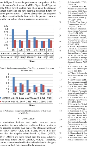
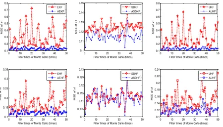
where NMCis the number of Monte Carlo simulations. Figure 1-Figure 2 shows the performance comparison of the filters in terms of their mean of MSEs. Figure 3 and Figure 4 plot the MSEs for 50 random runs when using the standard nonlinear filters and the new adaptive nonlinear filters for incorrect process noise. It shows clearly that the proposed new adaptive method is the best choice for practical cases in which the real values of noise variances are unknown.
V. CONCLUSION
The simulations indicate that under incorrect noise information, the new adaptive nonlinear filters provide a more accurate estimate than that of the standard nonlinear filters (EKF, SDKF, UKF, EHF, SDHF, UHF). It is also shown that the adaptive robust-based Hfilters (AEHF, ASDHF, AUHF) are more robust than the usual adaptive kalman-based filters (AEKF, ASDKF, AUKF). Therefore, less noise contaminated residuals can be obtained to design a more accurate fault detection and isolation system.
REFERENCES
[1] A. H. Jazwinski. (1970). Stochastic Processes and Filtering Theory. 64.
[2] C. G. Hilborn and D. G. Lainiotis, "Optimal Estimation in the Presence of Unknown Parameters," Systems Science and Cybernetics, IEEE Transactions on, vol. 5, pp. 38-43, 1969. [3] D. L. Alspach, et al., "A Bayesian solution to the problem of
state estimation in an unknown noise environment†,"
International Journal of Control, vol. 19, pp. 265-287, 1974/02/01 1974.
[4] T. Bohlin, "Four Cases of Identification of Changing Systems,"
Computational Methods for Modeling of Nonlinear Systems, vol. 126, p. 441, 1976.
[5] R. Kashyap, "Maximum likelihood identification of stochastic linear systems," Automatic Control, IEEE Transactions on, vol. 15, pp. 25-34, 1970.
[6] K. Myers and B. Tapley, "Adaptive sequential estimation with unknown noise statistics," Automatic Control, IEEE Transactions on, vol. 21, pp. 520-523, 1976.
[7] A. H. Jazwinski, "Adaptive filtering," Automatica, vol. 5, pp. 475-485, 1969.
[8] R. Mehra, "Approaches to adaptive filtering," Automatic Control, IEEE Transactions on, vol. 17, pp. 693-698, 1972. [9] R. Mehra, "On the identification of variances and adaptive
Kalman filtering," Automatic Control, IEEE Transactions on,
vol. 15, pp. 175-184, 1970.
[10] B. Carew and P. Belanger, "Identification of optimum filter steady-state gain for systems with unknown noise covariances,"
Automatic Control, IEEE Transactions on, vol. 18, pp. 582-587, 1973.
[11] B. J. Odelson, et al., "A new autocovariance least-squares method for estimating noise covariances," Automatica, vol. 42, pp. 303-308, 2006.
[12] M. Viberg, "Subspace-based methods for the identification of linear time-invariant systems," Automatica, vol. 31, pp. 1835-1851, 1995.
[13] P. Van Overschee and B. De Moor, "A unifying theorem for three subspace system identification algorithms," in American Control Conference, 1994, 1994, pp. 1645-1649 vol.2. [14] G. E. P. Box, et al., Time series analysis: forecasting and
control vol. 734: Wiley, 2011.
[15] B. J. Odelson, "Estimating disturbance covariances from data for improved control performance," UNIVERSITY OF
WISCONSIN, 2003.
[16] G. A. Einicke and L. B. White, "Robust extended Kalman filtering," Signal Processing, IEEE Transactions on, vol. 47, pp. 2596-2599, 1999.
[17] W. Li and Y. Jia, "H-infinity filtering for a class of nonlinear discrete-time systems based on unscented transform," Signal Processing, vol. 90, pp. 3301-3307, 2010.
[18] S. Xuemin and D. Li, "A dynamic system approach to speech enhancement using the H<sub>∞</sub> filtering algorithm," Speech and Audio Processing, IEEE Transactions on, vol. 7, pp. 391-399, 1999.
[19] D. Labarre, et al., "Dual H∞ Algorithms for Signal Processing- Application to Speech Enhancement," Signal Processing, IEEE Transactions on, vol. 55, pp. 5195-5208, 2007.
[20] G. Sibley, et al., "The iterated sigma point kalman filter with applications to long range stereo," in Proceedings of Robotics: Science and Systems, 2006, pp. 263-270.
[21] A. Mohamed and K. Schwarz, "Adaptive Kalman filtering for INS/GPS," Journal of Geodesy, vol. 73, pp. 193-203, 1999. [22] A. Jazwinski and A. Bailie, "Adaptive filtering Interim report,"
NASA Technical Reports (March 1, 1967)1967.
EKF SDKF UKF EHF SDHF UHF
Standard 2.5732 1.602 2.0304 1.2238 1.361 0.58 Adaptive 0.9552 1.3037 0.489 0.92 1.2501 0.457
0 0.5 1 1.5 2 2.5 3
M
ea
n
of
M
SE
s
Filters
EKF SDKF UKF EHF SDHF UHF
Standard 0.296 0.124 0.2869 0.1679 0.1113 0.146 Adaptive 0.1286 0.1146 0.1288 0.1215 0.1116 0.1199
0 0.05 0.1 0.15 0.2 0.25 0.3 0.35
M
ea
n
of
M
SE
s
[image:5.595.54.313.184.549.2]Filters
Figure 1. Performance comparison of the filters in terms of their mean of MSEs for x1
Figure 3. MSE for state x1across 50 random runs
Figure 4. MSE for state x2 across 50 random runs
0 10 20 30 40 50
0.1 0.2 0.3 0.4 0.5 0.6 0.7 0.8
Filter times of Monte Carlo (times)
M
S
E
o
f
x
1
EKF AEKF
0 10 20 30 40 50
0.1 0.11 0.12 0.13 0.14 0.15
Filter times of Monte Carlo (times)
M
S
E
o
f
x
1
SDKF ASDKF
0 10 20 30 40 50
0.1 0.2 0.3 0.4 0.5 0.6 0.7 0.8
Filter times of Monte Carlo (times)
M
S
E
o
f
x
1
UKF AUKF
0 10 20 30 40 50
0.1 0.15 0.2 0.25 0.3 0.35
Filter times of Monte Carlo (times)
M
S
E
o
f
x
1
EHF AEHF
0 10 20 30 40 50
0.1 0.105 0.11 0.115 0.12 0.125 0.13
Filter times of Monte Carlo (times)
M
S
E
o
f
x
1
SDHF ASDHF
0 10 20 30 40 50
0.1 0.12 0.14 0.16 0.18 0.2 0.22 0.24
Filter times of Monte Carlo (times)
M
S
E
o
f
x
1
UHF AUHF
0 10 20 30 40 50
0 1 2 3 4 5 6 7
Filter times of Monte Carlo (times)
M
S
E
o
f
x
2
EKF AEKF
0 10 20 30 40 50
0.8 1 1.2 1.4 1.6 1.8 2 2.2
Filter times of Monte Carlo (times)
M
S
E
o
f
x
2
SDKF ASDKF
0 10 20 30 40 50
0 1 2 3 4 5 6
Filter times of Monte Carlo (times)
M
S
E
o
f
x
2
UKF AUKF
0 10 20 30 40 50
0.5 1 1.5 2 2.5 3
Filter times of Monte Carlo (times)
M
S
E
o
f
x
2
EHF AEHF
0 10 20 30 40 50
0.8 1 1.2 1.4 1.6 1.8 2
Filter times of Monte Carlo (times)
M
S
E
o
f
x
2
SDHF ASDHF
0 10 20 30 40 50
0.2 0.4 0.6 0.8 1 1.2 1.4 1.6
Filter times of Monte Carlo (times)
M
S
E
o
f
x
2