Abstract robust coarse spaces for systems of PDEs via generalized eigenproblems in the overlaps

Numer. Math.

DOI 10.1007/s00211-013-0576-y

Numerische

Mathematik

Abstract robust coarse spaces for systems of PDEs via

generalized eigenproblems in the overlaps

N. Spillane · V. Dolean · P. Hauret · F. Nataf· C. Pechstein · R. Scheichl

Received: 31 October 2011 / Revised: 17 December 2012 © Springer-Verlag Berlin Heidelberg 2013

Abstract Coarse spaces are instrumental in obtaining scalability for domain

decom-position methods for partial differential equations (PDEs). However, it is known that most popular choices of coarse spaces perform rather weakly in the presence of hetero-geneities in the PDE coefficients, especially for systems of PDEs. Here, we introduce in a variational setting a new coarse space that is robust even when there are such heterogeneities. We achieve this by solving local generalized eigenvalue problems in

N. Spillane (

B

Laboratoire Jacques-Louis Lions, CNRS UMR 7598, Université Pierre et Marie Curie, 75005 Paris, France e-mail: [email protected]

F. Nataf

e-mail: [email protected] V. Dolean

Laboratoire J.-A.. Dieudonné, CNRS UMR 7351,

Université de Nice-Sophia Antipolis, 06108 Nice Cedex 02, France e-mail: [email protected]

P. Hauret

Centre de Technologie de Ladoux, Manufacture des Pneumatiques Michelin, 63040 Clermont-Ferrand Cedex 09, France

e-mail: [email protected] C. Pechstein

Institute of Computational Mathematics, Johannes Kepler University, Altenberger Str. 69, 4040 Linz, Austria

e-mail: [email protected] R. Scheichl

the overlaps of subdomains that isolate the terms responsible for slow convergence. We prove a general theoretical result that rigorously establishes the robustness of the new coarse space and give some numerical examples on two and three dimensional heterogeneous PDEs and systems of PDEs that confirm this property.

Keywords Coarse spaces·Overlapping Schwarz method·Two-level methods· Generalized eigenvectors·Problems with large coefficient variation

Mathematics Subject Classification (2000) 65F10·65N22·65N30·65N55

1 Introduction

The effort to achieve scalability in domain decomposition methods has led to the design of so called two-level methods. Each of these methods is characterized by two ingredients: a coarse space and a formulation of how this coarse space is incorporated into the domain decomposition method. We will work in the already extensively studied framework of the overlapping additive Schwarz preconditioner [29,31], and focus on the definition of a suitable coarse space with the aim to achieve robustness with respect to heterogeneities in any of the coefficients in the PDEs. Heterogeneous problems arise in many applications, such as subsurface flow or linear elasticity. One way to avoid long stagnation in Schwarz methods is to build the subdomains in such a way that the variations in the coefficients are small or nonexistent inside each subdomain. In this context, classical coarse spaces based on these subdomain partitions are known to be robust, see e.g. [5,6,9,10,21]. In many cases, this is not feasible and so recently, for scalar elliptic problems, these results have been extended to operator dependent coarse spaces and to coefficients that are not resolved by the subdomain partition, see e.g. [7,8,12,14–16,24,27,28], as well as [32] and the references therein.

A very useful tool for building coarse spaces for which the corresponding two-level method is robust, regardless of the partition into subdomains and of the coefficient distribution, is the solution of local generalized eigenvalue problems. They allow to select suitable coarse vectors that satisfy certain local stability estimates and guarantee that the selected coarse vectors are orthogonal. This idea was first used in the pioneer-ing work [2] within the multigrid community and the same ideas were incorporated into the spectral Algebraic Multigrid Method [3,13]. In the framework of two level additive Schwarz methods, [14,16,27] identify the bottleneck for proving a conver-gence bound which is independent of the jumps in the coefficients to be the so called stable decomposition property. For the scalar elliptic (Darcy) problem, [14] succes-fully proposes to solve local generalized eigenvalue problems on overlapping coarse patches that identify the modes that must be put into the coarse space in order for the stable splitting property to hold. The local coarse spaces are then ‘glued together’ via a partition of unity to obtain a global coarse space.

use multiscale partition of unity functions to eliminate some of the ‘bad’ eigenmodes a priori. While very effective in the scalar elliptic case, this may prove tricky in cases where there are several PDEs with several jumping coefficients. In the same context of the scalar elliptic equation, [7,8] propose a different generalized eigenvalue problem, associated with the Dirichlet-to-Neumann map, which is posed only on the boundary of each subdomain. In this aproach, the interior degrees of freedom in each subdo-main are eliminated leaving only those that are shared with neighbouring subdosubdo-mains, reducing the problem of finding the components that locally slow down convergence to eigenproblems on the interfaces. Introduced first in [8,22], this approach was rig-orously analysed in [7]. The proof relies on uniform (in the coefficients) weighted Poincare inequalities [25]. While this allows full robustness for the small overlap case (cf. [7]), in a completely general setting it has two drawbacks: (i) for larger overlap some assumptions are needed on the coefficient distribution in the overlaps and (ii) the arguments cannot be generalized easily to the case of systems of PDEs. It is in fact not essential to construct the orthogonal local coarse bases via generalized eigenproblems. In [28], an abstract Bramble-Hilbert lemma is proved that opens up the possibility for a whole range of other local functionals to achieve stability.

In this article, we propose a coarse space construction based on Generalized

Eigen-problems in the Overlap (which we will refer to as the GenEO coarse space). The

method was first and briefly introduced in [30] by the same authors and we give here a detailed proof of the previously stated convergence result along with some numerical results. The coarse space construction applies to systems of PDEs discretized by finite elements with only a few extra assumptions. It only relies on having access to element stiffness matrices and the connectivity graph between elements. The subdomain par-tition is carried out using Metis. Overlap is added based on the connectivity graph and the coarse space is constructed automatically solving a generalized eigenproblem on each subdomain. In our analysis, we identify that in the small overlap case the abstract Schwarz framework allows to reduce the stability condition to an energy bound in the overlap, and thus the second matrix in the pencil of our generalized eigenvalue problem is a matrix that has zero blocks corresponding to the interior of the subdomain at hand. The resulting generalized eigenvalue problems are closely related, but different to the ones proposed in [12]. Therefore the analysis and the final estimate are also different. In particular, the approach in [12] focuses on the generous overlap case. It requires a hexahedral coarse mesh and a procedure for computing multiscale partitions of unity subordinate to this coarse mesh. While it is clear that this is not a fundamental requirement in [12], and that their method could also be extended to the small overlap case and to more general coarse meshes, the same could be said about the GenEO coarse space. For implementational convenience we choose simple partition of unity operators that are sufficient in the small overlap case, but for larger overlap we could also use multiscale partitions of unity. Secondly (as in [12]), the requirement that the overlapping subdomains coincide with the supports of the coarse space partition of unity is not essential (cf. [27] in the case of our approach). Which of the two approaches is better in practice in terms of stability versus coarse space size is still the object of ongoing research. The recent work of [33] is a first step.

abstract variational setting that unfortunately does not allow for finite element spaces, since [12, Assumption A4(c)] cannot be satisfied in that case. In order for the proof to go through for classical finite element spaces, a stable interpolation operator with a constant independent of the coefficients would be needed. In many cases (elasticity for instance), such a stable interpolator does not yet exist to our knowledge. We over-came this problem by introducing partition of unity operators that work directly on the degrees of freedom instead of partition of unity functions. From a practical point of view, thanks to the partition of unity operators, the right hand side of the generalized eigenproblems can be constructed fully automatically from element stiffness matrices and diagonal weighting matrices. We only require access to some topological infor-mation to build a suitable partition of unity, as well as to the element stiffness matrices (as in AMGe methods, cf. [3]). This is reasonable in standard FE packages such as FreeFEM++ [17].

The rest of this article is organized as follows. In Sect.2 we define the problem that we solve and introduce the two-level additive Schwarz framework along with some elements of generalized eigenvalue problem theory. In Sect.3 we define the abstract procedure to construct our coarse space and give the main convergence result (Theorem3.22).

Section4gives detailed guidelines on how to implement the two-level Schwarz pre-conditioner with the GenEO coarse space in a finite element code. Finally in Sect.5we test our method for Darcy and linear elasticity and make sure that it indeed converges robustly even for highly varying coefficients in two and three dimensions.

2 Preliminaries and notations

2.1 Problem description

Given a Hilbert space V , a symmetric and coercive bilinear form a:V×V →Rand an element f in the dual space V, we consider the abstract variational problem: Find

v∈V such that

a(v, w)= f, w, for all w∈V, (2.1)

where·,·denotes the duality pairing. This variational problem is associated with an elliptic boundary value problem (BVP) on a given domainΩ ⊂Rd(d =2 or 3) with suitable boundary conditions posed in a suitable space V of functions onΩ.

We consider a discretization of the variational problem (2.1) with finite elements based on a meshThofΩ:

Ω =_τ∈Thτ.

Let Vh ⊂V denote the chosen conforming space of finite element functions. In the

case where a(·,·)is a bilinear form derived from a system of PDEs, Vhis a space of vector functions. The discretization of (2.1) then reads: Findvh ∈Vhsuch that

Let{φk}n_k=1be a basis for Vhwith n:=dim(Vh), then from (2.2) we can derive a linear system

Av = f, (2.3)

where the coefficients of the stiffness matrix A∈Rn×n_{and the load vector f ∈R}n_are given by Ak_,l =a(φl, φk)and fk = f, φk, where k, l =1, . . . ,n, and v is the vector of coefficients corresponding to the unknown finite element functionvhin (2.2).

The basis{φk}n_k=1 can be quite arbitrary but it should fulfil a unisolvence prop-erty, such that the basis functions supported on each element τ ∈ Th are linearly independent when restricted toτ. This is the case for standard finite element bases.

The only significant assumption we make on the problem is that the stiffness matrix

A is assembled from positive semi-definite element stiffness matrices.

Assumption 2.1 Let Vh(τ) = {v|τ : v ∈ Vh}. We assume that there exist positive semi-definite bilinear forms a_τ :Vh(τ)×Vh(τ)→R, for allτ ∈Th, such that

a(v, w)= τ∈Th

a_τ(v|_τ, w|_τ), for all v, w∈Vh.

Remark 2.2 If the variational problem is obtained from integrating local forms on the

domain then this is not a problem at all. For instance in the case of the Darcy equation we can write for allv, w∈ H₀1(Ω):

a(v, w)=

Ω

κ∇v· ∇w= τ∈Th

τ

κ∇v· ∇w= τ∈Th

a_τ(v|_τ, w|_τ).

2.2 Additive Schwarz setting

In order to automatically construct a robust two-level Schwarz preconditioner for (2.3), we first partition our domainΩ into a set of non-overlapping subdomains{Ω_j}N_j=1 resolved byThusing for example a graph partitioner such as METIS [18] or SCOTCH [4]. Each subdomainΩ_j is then extended to a domainΩj by adding one or several layers of mesh elements in the sense of Definition2.3, thus creating an overlapping decomposition{Ωj}N_j=1ofΩ.

Definition 2.3 Given a subdomain D ⊂Ω which is resolved byTh, the extension of Dby one layer of elements is

D=Int

⎛

⎝

{k:supp(φk)∩D=∅}

supp(φk)

⎞ ⎠

The proof of the following lemma is a direct consequence of Definition2.3.

Lemma 2.4 For every degree of freedom k, with 1≤k≤n, there is a subdomainΩj,

with 1≤ j ≤N , such that supp(φk)⊂Ωj.

Now, for each j =1, . . . ,N , let

Vh(Ωj):= {v|Ωj :v∈Vh}

denote the space of restrictions of functions in VhtoΩj. Furthermore, let

Vh,0(Ωj):= {v|Ωj :v∈Vh, supp(v)⊂Ωj}

denote the space of finite element functions supported inΩj. By definition, the exten-sion by zero of a functionv ∈Vh,0(Ωj)toΩ lies again in Vh. We denote the corre-sponding extension operator by

R_j :Vh,0(Ωj)→Vh. (2.4)

Lemma2.4guarantees that Vh=N_j=1R_jVh,0(Ωj). The adjoint of Rj

Rj :Vh →Vh,0(Ωj),

called the restriction operator, is defined byRjg, v = g,Rjv, forv∈ Vh,0(Ωj),

g ∈V_h. However, for the sake of simplicity, we will often leave out the action of R_j and view Vh,0(Ωj)as a subspace of Vh.

The final ingredient is a coarse space VH ⊂ Vh which will be defined later. Let

R_H :VH →Vhdenote the natural embedding and RHits adjoint. Then the two-level additive Schwarz preconditioner (in matrix form) reads

M−_AS1_,2=RT_HA−_H1RH + N

j₌1

RT_jA−_j1Rj, AH:=RHARTH and Aj:=RjARTj, (2.5)

where Rj, RH are the matrix representations of Rj and RH with respect to the basis {φk}nk₌1and the chosen basis of the coarse space VH. As usual for standard elliptic

BVPs, Aj corresponds to the original (global) system matrix restricted to subdomain

Ωj with Dirichlet conditions on the artificial boundary∂Ωj\∂Ω. To simplify the notation, if D is the union of elements ofThand

Vh(D):= {v|D:v ∈Vh},

we write, for anyv, w∈Vh(D),

aD(v, w):=

τ∈D

a_τ(v|_τ, w|_τ) and |v|a_,D =

where the latter is the energy seminorm. The definition of aD(·,·)extends naturally tov, w ∈ Vh(D), for any D ⊂D ⊂Ω which simplifies notations. On each of the local spaces Vh,0(Ωj)the bilinear form aΩj(·,·)is positive definite since

a_Ωj(v, w)=a(R_jv,R_jw), for allv, w∈Vh,0(Ωj),

and because a(·,·)is coercive on V . For the same reason, the matrix Aj in (2.5) is invertible. Hence,| · |a_,Ωj becomes a norm on Vh,0(Ωj)and so we write

va,Ωj =

a_Ωj(v, v), for allv∈Vh,0(Ωj).

If D=Ω, we omit the domain from the subscript and write · ainstead of · a_,Ω. We use here the abstract framework for additive Schwarz (see [31, Chapter 2]). In the following we summarize the most important ingredients.

Definition 2.5 We define k0=max_τ∈Th

#{Ωj :1≤ j ≤N, τ ⊂Ωj}

.

This means that each point inΩ belongs to at most k0of the subdomainsΩj.

Lemma 2.6 With k0as in Definition2.5, the largest eigenvalue of M−_AS1_,2A satisfies

λmax

M−_AS1_,2A

≤ k0+1.

Proof See, e.g., [11, Section 4].

Definition 2.7 (Stable decomposition) Given a coarse space VH ⊂ Vh, local sub-spaces{Vh,0(Ωj)}1≤j≤N and a constant C0, a C0-stable decomposition ofv ∈Vhis a family of functions{zj}0≤j≤Nthat satisfies

v= N

j=0

zj, with z0∈VH, zj ∈Vh,0(Ωj), for j≥1, (2.6)

and

z02a+ N

j=1

_zj2

a,j ≤C

2

0v2a . (2.7)

Theorem 2.8 If everyv∈ Vhadmits a C0-stable decomposition (with uniform C0),

then the smallest eigenvalue of M−_AS1_,2A satisfies

λmi n(M−AS1_,2A) ≥ C− 2 0 .

Therefore, the condition number of the two-level Schwarz preconditioner (2.5) can be

bounded by

Proof The statement is a direct consequence of [31, Lemma 2.5] and Lemma2.6.

In the following, we will construct a C0-stable decomposition in a specific

frame-work, but prior to that we will provide in an abstract setting, a sufficient and simplified condition of stability.

Lemma 2.9 Using the notations introduced in Definition2.7, if there exists a constant

C1such that

zj2a,Ωj ≤C1|v|

2

a,Ωj for all j =1, . . . ,N, (2.8)

then the decomposition (2.6) is C0-stable with C₀2=2+C1k0(2k0+1)where k0is

given in Definition2.5.

Proof From (2.8) and Definition2.5we get successively

N

j=1

_zj2

a,j ≤C1

N

j=1

|v|2

a,j ≤C1k0v

2

a. (2.9)

We also have:

z02a=

v−

N

j=1

zj 2 a

≤2v2_a+2

N

j=1

zj 2 a , (2.10)

and from Definition2.5and (2.9) we get

N

j=1

zj 2 a ≤k0

N

j=1

zj

2

a,j ≤C1k

2 0v

2

a. (2.11)

Using (2.11) in (2.10) yields

z02a≤2(1+C1k20)v2a. (2.12)

By adding (2.9) and (2.12) we get (2.7) with C₀2=2+C1k0(2k0+1).

Whenz02acan be bounded directly in terms ofv2a(independently of the coeffi-cient variation), this lemma is superfluous and leads to a suboptimal quadratic depen-dence on k0. In general, however, it is not possible to provide such a uniform bound

2.3 Abstract generalized eigenproblems

In order to construct the coarse space we will use generalized eigenvalue problems in each subdomain. Since several variations of generalized eigenvalue problems exist in the literature (particularly concerning the interpretation of the ‘infinite eigenvalue’), we state the definition that we use.

Definition 2.10 (Generalized eigenvalue problem) Let V be a finite-dimensional

Hilbert space, leta :V×V→ Randb : V ×V → Rbe two symmetric bilinear forms. Then the generalized eigenvalues associated with the so called ‘pencil’(a,b)

are the following valuesλ ∈ R∪ {+∞}: eitherλ ∈ Rand there exists p ∈ V\{0}

such that

a(p, v)=λb(p, v), for allv∈V, (2.13)

orλ= +∞and there exists p∈V\{0}such that

b(p, v)=0, for allv∈V, and a(p, v)=0, for a certain v∈V.

In both cases p is called a generalized eigenvector associated with the eigenvalueλ. The definition above allows for infinite eigenvalues. This results from the fact that if(+∞,p)is an eigenpair for the pencil(a,b)then(0,p)is an eigenpair for the pencil(b,a)and there is no reason to discriminate between both formulations. In cases where the bilinear formb is positive definite, the problem can be simplified

and crucial properties on the eigenvalues and eigenvectors arise. In particular, it leads quite naturally to optimal projectors onto subspaces of the functional space, as the next lemma shows in an abstract setting.

Lemma 2.11 Leta be positive semi-definite and˜ b positive definite, and let the eigen-˜

pairs{(pk, λk)}kdim=1(V)of the generalized eigenvalue problem (2.13) be ordered such

that

0≤λ1≤. . .≤λdim(V) and b(pk,pl)=δkl, for any 1≤k,l ≤dim(V).

Then, for any integer 1≤m<dim(V), the projection

Πmv:= m

k=1

b(v,pk)pk

isa-orthogonal, and thus

|Πmv|a≤ |v|a and |v−Πmv|a≤ |v|a, for allv∈V. (2.14)

Additionally, if m is such thatλm+1>0, we have the stability estimate

v−Πmv2_b ≤ 1

λm+1|v−

Proof Due to the additional assumptions ona andb, the generalized eigenvalue

prob-lem can be simplified to a standard eigenvalue probprob-lem, for which the existence of eigenvectors{pk}dim_k=1(V) with associated non-negative real eigenvalues{λk}dim_k=1(V) is guaranteed by standard spectral theory. Moreover,{pk}dim_k=1(V)can be chosen such that it is a basis ofV fulfilling the orthogonality conditions:

a(pk,pl)=b(pk,pl)=0 ∀k=l, |pk|2_b=1 and |pk|2a=λk.

Now letv∈V be fixed. From the b-orthonormality of the basis we get

v=

dim(V) k=1

b(v,pk)pk.

For any index set I ⊂ {1, ...,dim(V)}, thea-orthogonality implies

k∈I

b(v,pk)pk

2 a

=

k∈I

b(v,pk)2|pk|2a.

Thus

|v|2

a= |Πmv|2a+ |v−Πmv|2a. and (2.14) follows directly. Finally,

v−Πmv2_b=

dim(V) k=m+1

b(v,pk)pk

2

b

=

dim(V) k=m+1

b(v,pk)2 (by theb−orthonormality of pk)

=

dim(V) k=m+1

b(v,pk)2 1

λk|

pk|_a2 (sinceλk = |pk|2a)

≤ 1

λm+1 dim(V) k=m+1

b(v,pk)2|pk|2a (sinceλ1≤. . .≤λdim(V))

= _λ1 m+1|v−

Πmv|2a (by thea−orthogonality of pk).

space and the local subspaces. It is in fact the central part in all the approaches that relie on solving eigenvalue problems, cf. Lemma 3.2 in the pioneering work [2] where b is the l2(euclidean) inner product or Eq. (2.8) in [12] where b is a particular bilinear form

defined there. The particular form of b is one of the defining elements that characterizes each of these methods and for GenEO it will be introduced in the next section.

3 Algebraic construction of a robust coarse space and its analysis

In this section we introduce the coarse space and give a bound on the condition number of the two-level additive Schwarz method with this coarse space along with a rigorous proof of this result. The proof will consist in proving the existence of a stable splitting for any function in Vhin the sense of Definition2.7.

3.1 The coarse space

The GenEO coarse space is constructed as follows. In each subdomain we pose a suitable generalized eigenproblem and select a number of low frequency eigenfunc-tions. These local functions are converted into global coarse basis functions using a partition of unity operator. As mentioned before, the eigenproblems are restricted to the overlapping zone, which is introduced in the next definition. Following this def-inition, we will then define the partition of unity operator, which will appear both in the eigenproblems themselves and in the construction of the coarse basis functions.

Definition 3.1 (Overlapping zone) For each subdomainΩj (1≤ j ≤N ), the over-lapping zone is given by

Ω◦j = {x∈Ωj : ∃j= j such that x ∈Ωj}.

We will also require the set of degrees of freedom associated with Vh(Ωj), as well as those associated with Vh_,0(Ωj), for 1≤ j ≤N .

Definition 3.2 Given a subdomain D that is a union of elements fromTh, let

dof(D):= {k=1, . . . ,n :supp(φk)∩D= ∅}

denote the set of degrees of freedom that are “active” in D, including those associated with the boundary. Similarly, we denote by

dof(D):= {k: 1≤k≤n and supp(φk)⊂D}

the set of internal degrees of freedom in D.

Remark 3.3 Since the basis functionsφk of Vhfulfil a unisolvence property on each

element they also fulfil a unisolvence property on each subdomain Ωj, in other words the functions{φk|_Ωj}_k∈dof(Ωj)(resp.{φk|_Ωj}k_∈dof_(Ωj)) are linearly independent.

Now we can introduce the partition of unity operators. Recall that, for anyv∈Vh, we writev=nk₌1vkφk.

Definition 3.4 (Partition of unity) For each degree of freedom k ∈ dof(Ω):= {1,

. . . ,n}, let{μj,k :k∈dof(Ωj), 1≤ j≤ N}be a family of weights such that

μj,k≥1 and

{j;k∈dof(Ωj)}

1

μj,k = 1.

Then, for 1≤ j ≤N , the local partition of unity operatorΞj :Vh(Ωj)→Vh,0(Ωj) is defined by

Ξj(v) :=

k∈dof(Ωj)

1

μj,kv

kφk|_Ωj, for allv∈Vh(Ωj).

Remark 3.5 A possible choice for the weights in Definition3.4is to use the multiplicity

of each degree of freedom: for any degree of freedom k∈dof(Ω), letμkdenote the number of subdomains for which k is an internal degree of freedom, i.e.

μk:=#{j : 1≤ j ≤ N and k∈dof(Ωj)}

and then use the equal weightsμj,k:=μk, for any j =1, . . . ,N with k ∈dof(Ωj).

Lemma 3.6 The operators Ξj from Definition3.4form a partition of unity in the

following sense:

N

j=1

R_j Ξj(v|Ωj) = v, for allv∈Vh. (3.1)

Moreover,

Ξj(v)|Ωj\Ω◦j =v|Ωj\Ωj◦, forallv∈Vh(Ωj) and 1≤ j≤ N. (3.2)

Proof Property (3.1) follows directly from the definition. To show (3.2), let v ∈

Vh(Ωj)and recall that by definition

Ξj(v)|_Ωj\Ω◦j =

k∈dof(Ωj)

1

μj,kv

kφk|_Ωj\Ω◦

j .

Now note that ifμj,k >1, thenφk|_Ωj\Ω◦

j = 0, because k ∈ dof(Ω

j)for j = j. Hence,

Ξj(v)|Ωj\Ω◦j =

k∈dof(Ωj)s.t. μj,k=1

vkφk|_Ωj\Ω◦j =

k_∈dof_(Ωj\Ω◦j)

vkφk|_Ωj\Ω◦j ,

Next we define the local generalized eigenproblems for the GenEO coarse space.

Definition 3.7 (Generalized eigenproblems in the overlaps) For each j=1, . . . ,N ,

we define the following generalized eigenvalue problem

a_Ωj(p, v)=λbj(p, v), for all v∈Vh(Ωj). (3.3)

where bj(p, v):=a_Ω◦_j(Ξj(p), Ξj(v)), for all p, v∈Vh(Ωj).

Remark 3.8 Although the form of the bilinear forms bj(·,·)seems somewhat artificial,

we will see below that it actually arises naturally in the analysis. It is clear that the actual eigenvalues and eigenvectors will depend on the choice of the partition of unity in Definition3.4.

The GenEO coarse space is now constructed (locally) as the span of a suitable subset of the eigenfunctions in (3.3). Finally, to obtain a global coarse space we apply the partition of unity operators.

Definition 3.9 (GenEO coarse space) For each j = 1, . . . ,N , let(p_kj)m_k=j₁be the eigenfunctions of the eigenproblem (3.3) in Definition3.7corresponding to the mj smallest eigenvalues. Then,

VH:=span{RjΞj(pkj):k=1, . . . ,mj; j =1, . . . ,N},

where Ξj are the partition of unity operators from Definition3.4 and R_j are the extension operators defined in (2.4).

Consequently, we can also make explicit the final component in Definition2.5of the matrix form M−_AS1_,2of the additive Schwarz preconditioner, namely the prolongation matrix RT_H. The columns of the rectangular matrix RT_H ∈Rn×dim(VH)_{are simply the}

vector representations of the functions{R_jΞj(p_kj):k=1, . . . ,mj; j =1, . . . ,N} with respect to the finite element basis{φk}n_k=1. Clearly dim(VH)=Nj=1mj and a strategy for selecting mjwill be given below. This completes the definition of M−_AS1_,2.

3.2 Analysis of the preconditioner

To confirm the robustness of the above coarse space and to bound the condition number of M−_AS1_,2A via Theorem2.8we will now show that there is a stable splitting for each

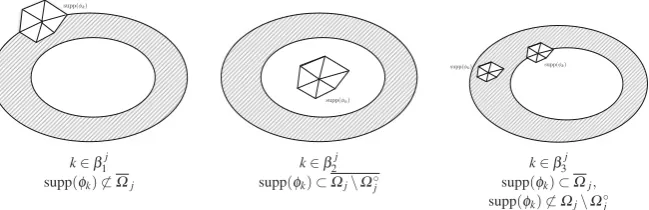
Fig. 1 Three types of finite element basis functions on each subdomainΩj. The hashed surface is the overlapΩ◦_j

Definition 3.10 We partition the set dof(Ωj)of degrees of freedom in Vh(Ωj)into three sets (see also Fig.1):

βj

1:=dof(Ωj)\dof(Ωj) (the DOFs on the boundary ofΩj),

βj

2:=dof(Ωj\Ω◦j) (the interior DOFs inΩj\Ω◦j),

βj

3:=dof(Ωj)\dof(Ωj\Ω◦j) (the DOFs in the overlap, incl. the inner boundary). From these index sets we define subsets of functions of Vh(Ωj)

Bj

1:=span

φk|_Ωj

k∈β₁j , B j

2:=span

φk|_Ωj

k∈β₂j and B j

3:=span

φk|_Ωj

k∈β₃j,

such that

Vh(Ωj)=B₁j⊕B₂j ⊕B₃j.

The following simple properties will be used frequently in the following.

Lemma 3.11 For any 1≤ j ≤N , the following properties are true

1. supp(v)⊂Ω◦_j, for allv∈B₁j,

2. B₁j =Ker(Ξj),

3. B₂j = {v∈Vh(Ωj):v|Ω◦_j =0},

4. a_Ωj is coercive onB₂j.

Proof 1. For any basis functionφk with k ∈ β1j, Lemma2.4implies that there is

another subdomainΩj with supp(φk)⊂Ωj, and so supp(φk)∩(Ωj\Ω◦_j)= ∅. 2. Letv∈Vh(Ωj). Then

v∈Ker(Ξj)⇔vk=0, for all k ∈dof(Ωj)⇔v=

k∈β₁j

3. It is clear from the definition of B₂j that B₂j ⊂ {v ∈ Vh(Ωj) : v|Ω◦_j = 0}. Conversely, ifv|_Ω◦

j = 0, then from the unisolvence property, vk = 0, for all k∈dof(Ω◦_j)=β₁j ∪β₃j, and therefore{v∈Vh(Ωj):v|Ω◦_j =0} ⊂B2j also.

4. The previous property implies thatB₂j ⊂Vh,0(Ωj)and so

a_Ωj(v, w)=a(R_jv,R_jw) for allv, w∈B₂j.

The coercivity of a_Ωj(·,·)onB

j

2follows from the coercivity of a(·,·).

To carry out a robustness analysis we need to make the following two assumptions.

Assumption 3.12 For any 1≤ j≤ N , a_Ωj is coercive onB

j

1. Assumption 3.13 For any 1≤ j≤ N , a_Ω◦

j is coercive onB

j

3.

Note that by the first property in Lemma3.11, Assumption3.12is equivalent to assuming that, for any 1≤ j ≤N , a_Ω◦

j is coercive onB

j

1.

Remark 3.14 Assumptions3.12 and3.13 are not too restrictive. If all the element

stiffness matrices are positive definite, then a_Ωj and aΩ◦j are positive definite on the

whole of Vh(Ωj). For the Darcy equation or linear elasticity, the element stiffness matrices are not positive definite. However, any functionv∈B₁jsatisfiesvk =0, for

k ∈β₁j, and any functionv ∈ B₃j vanishes on the boundary ofΩj (i.e.vk =0, for

k∈β₁j). Therefore, in the Darcy case and in the case of standard H1-conforming finite elements, Assumptions3.12and3.13hold if each of the setsβ₁j andβ₃j contains at least one DOF. To make the assumptions hold for linear elasticity, the setsβ₁jandβ₃j need to contain enough DOFs to fix the rigid body modes inΩ◦_j, i.e., at least 3(d−1) DOFs. Hence, for standard H1_{-conforming finite elements, it is sufficient to have d}

non-collinear points (with associated DOFs for all components of the vector function) that lie on the outer boundary∂Ωj, respectively inΩ◦_j\∂Ωj.

The final technical hurdle to construct a stable splitting is that we cannot apply the abstract Lemma 2.11 to the specific eigenproblems used in the con-struction of the GenEO coarse space VH directly, because the bilinear forms

bj(·,·):=a_Ω◦_j(Ξj(·), Ξj(·))from Definition3.3are not necessarily positive definite on all of Vh(Ωj)×Vh(Ωj), for all 1≤ j≤ N . To complete the analysis we thus need to define a suitable subspaceVj ⊂Vh(Ωj)such that bjis positive definite onVj×Vj.

Definition 3.15 Let the spacesVj andWj be defined by

Vj:={v∈Vh(Ωj):aΩj(v, w)=0, for allw∈Wj} where Wj:=B

j

1⊕B

j

2. Lemma 3.16 Under Assumption3.12,

Proof Since a_Ωj is coercive on B

j

1 (cf. Assumption 3.12) and on B

j

2 (cf.

Lemma3.11(4)) and since functions inB₁j andB₂j have disjoint supports, we also have that a_Ωj is coercive onWj. It follows from the definition ofVj(via some simple

linear algebra) thatVj ∩Wj = {0}and that dim(Vj)= dim(Vh(Ωj))−dim(Wj).

Remark 3.17 While this lemma shows thatVj andB3j contain the same degrees of

freedom, it does not imply thatVj =B₃j. Indeed having chosen values for the degrees of freedom in β₃j, the corresponding function in Vj is the discrete PDE-harmonic extension to the whole ofΩjwhile the corresponding function inB3jis the extension

by zero. The discrete harmonic extension intoΩj\Ω◦j is always well defined because of the coercivity of a_ΩjonB

j

2(cf. Lemma3.11(4)). The fact that the discrete harmonic

extension ontoB₁j is well defined is a consequence of Assumption3.12. The role of Assumption3.13becomes clear in the next lemma.

Lemma 3.18 Under Assumptions3.12and3.13, for j =1, ...,N , the bilinear form

bj(·,·):=aΩ◦_j(Ξj(·), Ξj(·))is positive definite onVj ×Vj.

Proof Letv∈Vj such thatbj(v, v)=0. We need to show that necessarilyv=0.

There exists a unique decompositionv =v1+v2+v3, such thatvi ∈ B_ij. The second property in Lemma3.11states thatB₁j =Ker(Ξj), and so

Ξj(v1)=0.

From the definition ofΞjit is obvious thatΞj|_Bj

2 :B

j

2 →B

j

2is the identity, and so

Ξj(v2)∈B₂j and in particular from the third property in Lemma3.11

supp(Ξj(v2))∩Ω◦j = ∅. From these two remarks and the definition of bj it follows that

bj(v, v)=a_Ω◦_j(Ξj(v3), Ξj(v3)). (3.4)

Moreover, from the definition of Ξj it is also obvious thatΞj|_Bj

3 : B

j

3 → B

j

3

is a bijection, and so Ξj(v3) ∈ B3j. Now, (3.4) and Assumption 3.13 imply that

Ξj(v3)= 0. The fact thatΞj|_Bj

3

is a bijection in turn implies thatv3 = 0, and so

v∈Wj. From Lemma3.16, we know thatVj∩Wj = {0}, and sov=0 which ends

the proof.

We can now apply Lemma2.11to the restriction of the GenEO eigenproblems to

Lemma 3.19 For each j =1, ...,N , consider the generalized eigenproblem (3.3) in

Definition3.7.

(i) There are dim(Vj)finite eigenvalues 0 ≤ λ1j ≤ λ

j

2 ≤ . . . ≤ λ

j

dim(Vj) < ∞ (counted according to multiplicity) with corresponding eigenvectors denoted by

{p_kj}dim_k=1(Vj) and normalized to form an orthonormal basis ofVj with respect to

bj(·,·).

(ii) There are dim(Wj)infinite eigenvaluesλ_dimj _(V

j)+1 = . . . =λ

j

dim(Vh(Ωj)) = ∞

with associated eigenvectors denoted by{p_kj}_dimdim(₍V_Vh(Ωj))

j)+1 forming a basis of

Wj.

Proof Since Vh(Ωj)=Vj⊕Wj (cf. Lemma3.16) and aΩj(v, w)=bj(v, w)=0,

for all v ∈ Vj andw ∈ Wj, the eigenproblem (3.3) can be decoupled into two eigenproblems: one onVj and one onWj.

Since, according to Lemma3.18, bj(·,·)is coercive onVj ×Vj, we can apply Lemma2.11withV→Vj,a→aΩj, andb→bj to analyse the restriction of (3.3)

toVj. This completes the proof of (i).

For the restriction of (3.3) toWj, we prove that all vectors inWjare eigenvectors associated with the eigenvalue+∞in the sense of Definition2.10. Letv∈Wj. Then

Ξj(v)|_Ω◦_j =0 and so in particular

a_Ω◦

j(Ξj(v), Ξj(w))=0 for allv, w∈Wj. (3.5)

Moreover, we have already seen in the proof of Lemma3.16that a_Ωj is coercive on

Wj, and so

aΩj(v, v)=0 for allv∈Wj\{0}. (3.6)

Due to (3.5) and (3.6), anyv∈Wj is indeed an eigenvector to the eigenvalue+∞in the sense of Definition2.10. We can use any set of linearly independent vectors inWj to form a basis, e.g.{p_kj}dim(Vh(Ωj))

k=dim(Vj)+1= {φk|Ωj}k∈β1j∪β

j

2

.

We are now ready to define the crucial projection operators onto the local compo-nents of the GenEO coarse space that satisfy suitable stability estimates.

Lemma 3.20 (Local stability estimate) Let j ∈ {1, ...,N}and let{(p_kj, λ_kj)}dim_k=1(Vh(Ωj))

be as defined in Lemma3.19. Suppose that mj ∈ {1, . . . ,dim(Vh(Ωj))−1}such that

0< λ_mj

j+1<∞. Then, the local projection operator

Πj mjv:=

mj

k=1

a_Ω◦

j(Ξj(v), Ξj(p

j k))p

satisfies

|Πj

mjv|a,Ωj ≤ |v|a,Ωj and |v−Π

j

mjv|a,Ωj ≤ |v|a,Ωj, for allv∈Vh(Ωj),

(3.7)

as well as the stability estimate

Ξj(v−Πmjjv) 2

a,Ω◦_j ≤ 1

λj mj+1

v−Πj

mjv 2

a,Ωj

, for allv∈Vh(Ωj). (3.8)

Proof The condition λ_mj _j+1 < ∞, ensures that mj ≤ dim(Vj), soΠmjj maps to

Vj. Therefore, for allv ∈ Vj, the estimates in (3.7) and (3.8) can be deduced from Lemma2.11again, withV→Vj,a→aΩj,b→bj, and m→mj.

To prove the result for allv∈Vh(Ωj), we use again the fact that Vh(Ωj)=Vj⊕Wj and that aΩj(v, w)=0, for allv∈Vjandw∈Wj. Letv=vV+vW ∈Vh(Ωj)with

vV ∈ Vj andvW ∈Wj. ThenΠmjjv =Π

j

mjvV and so (3.7) follows due to the aΩj

-orthogonality ofVjandWj. Estimate (3.8) follows similarly fromΞj(vW)|Ω◦_j =0.

Lemma 3.21 (Stable decomposition) Letv ∈ Vh and suppose the definitions and

notations of Lemma3.20hold. Then, the decomposition

z0:=

N

j=1

Ξj(Πmjjv|Ωj), zj:=Ξj(v|Ωj −Π

j

mjv|Ωj), for j=1, . . . ,N,

is C0-stable with

C₀2=2+k0(2k0+1) max

1≤j≤N

⎛

⎝1+ 1

λj mj+1

⎞ ⎠_.

Proof By definitionzj2_a,Ωj=|Ξj(v−Πmjjv|Ωj)|

2

a_,Ω◦_j+|Ξj(v−Π j mjv|Ωj)|

2

a_,Ωj\Ω◦j.

However, due to property (3.2) in Lemma3.6,Ξj is the identity for restrictions of functions toΩj\Ω◦j, and so

zj2a_,Ωj=Ξj(v−Π

j mjv|Ωj)

2

a,Ω◦_j + v−Π j mjv|Ωj

2

a,Ωj\Ω◦j .

Now we can apply Lemma3.20to get

zj2a,Ωj&≤ ⎛

⎝1+ 1

λj mj+1

⎞

⎠ _v−Πj mjv|Ωj

2

a,Ωj ≤ ⎛

⎝1+ 1

λj mj+1

⎞ ⎠_|v|2

a,Ωj,

With this stable decomposition we can now state our main result on the convergence of the two-level Schwarz preconditioner with the new GenEO coarse space. It follows immediately from Theorem2.8and Lemma3.21.

Theorem 3.22 (Bound on the condition number) Let Assumptions2.1,3.12, and3.13

hold. Suppose that the coarse space VH is given by Definition3.9and M−_AS1_,2is as

defined in (2.5).

Then we can bound the condition number for the two-level Schwarz method by

κ(M−_AS1_,2A) ≤ (1+k0)

2+k0(2k0+1) max 1≤j≤N

1+ 1

λj mj+1

,

where k0is given in Definition2.5.

The only parameters that need to be chosen in our coarse space are the numbers mj of eigenmodes on each subdomainΩj, 1≤ j ≤N , to be included in the coarse space. We suggest the following choice which recovers the condition number estimate for problems with no strong coefficient variation.

Corollary 3.23 For any j , 1≤ j ≤ N , let

mj := min

m:λ_mj₊₁> δj

Hj

, (3.9)

whereδj is a measure of the width of the overlapΩ◦_j and Hj =diam(Ωj). Then

κ(M−_AS1_,2A) ≤ (1+k0)

2+k0(2k0+1) max 1_≤j_≤N

1+ Hj

δj

.

Note that the number of subdomains and the coefficient variations do not appear in this bound on the condition number. This means that we have established rigorously that the algorithm is robust with respect to these two parameters. We will confirm this with some numerical tests in Sect.5. The size of the coarse space induced by the criterion does however depend on the geometry of the coefficient variation in the overlaps and the choice of the partition of unity. In fact, for some problems it may happen that even for a very small criterion the number of eigenmodes which are selected is very large. This is the case for instance in the context of linear elasticity when one of the materials is almost incompressible (i.e. its Poisson ration approaches 1/2), because then the bilinear form a_Ω◦

j(Ξj(·), Ξj(·)) on the right hand side of

eigenproblem (3.3) has very high energy.

4 Implementation

demonstrate below, our algorithm requires only abstract information of the problem in form of the element stiffness matrices and no further information on the mesh, the finite element spaces, or any coefficients. Indeed, for running the algorithm we need

(i) the list dof(τ)of degrees of freedom associated with each elementτ ∈Th, (ii) the element stiffness matrix Aτ = (a_τ(φl, φk))k,l∈dof(τ) associated with each

elementτ ∈Th.

Unless the overlapping subdomain partition is available a priori, we additionally need

(iii) the numberof layers which determine the amount of overlap.

Before going into details, we note that as for the classical two-level overlapping Schwarz method (see, e.g. [31, Sect. 3]), our algorithm can be parallelized straightfor-wardly. In particular, the solution of the eigenproblems in the preprocessing step and the subdomain solves during each PCG iteration can be performed fully in parallel.

4.1 Preprocessing

We need the overlapping partitionΩ = Nj=1Ωj in form of the list of elements associated with each subdomainΩj. To obtain this, we first create the connectivity graph of the elements (using the lists dof(τ)from (i)) and partition it into disjoint sets of elements which make up the non-overlapping subdomainsΩ_j using for instance METIS [18] or SCOTCH [4]. Then, for each (global) DOF k, we build the list

elem(k)= {τ ∈Th:k∈dof(τ)}

of elements where DOF k is active. This list realizes supp(φk)without knowing the basis functionφk itself. In a second step we addlayers to each non-overlapping subdomainΩ_j according to Definition2.3, which finally results in a list of elements per (overlapping) subdomainΩj. From this, we construct

dof(Ωj)=

τ⊂ ¯Ωj

dof(τ)

(cf. Definition3.2). Then we can compute the set of internal degrees of freedom in

Ωj

dof(Ωj)=

⎧ ⎨

⎩k∈dof(Ωj):

τ∈elem(k)

τ ⊂ ¯Ωj

⎫ ⎬ ⎭

4.2 The eigenproblems

For each subdomainΩj, j =1, . . . ,N we use a local renumbering of the degrees of freedom dof(Ωj)of Vh(Ωj). By assembling the element stiffness matrices for these DOFs over the elementsτ ⊂ ¯Ωj, we get the subdomain ”Neumann” matrixAj. This is the matrix formulation of a_Ωj(·,·): Vh(Ωj)×Vh(Ωj)→ R. For the same renumbering of DOFs, we assemble only over the elementsτ ⊂ ¯Ω◦_j in the overlap and obtain matrixA◦_j associated with the bilinear form a_Ω◦

j(·,·): Vh(Ωj)→ Vh(Ωj).

Note thatAj andA◦_j have the same format, butA◦_j usually contains a block of zeros corresponding to the degrees of freedom that are in the part of Ωj which is not overlapped by other subdomains.

From Definition3.4, we see immediately that the action of the operatorΞj can be coded by a diagonal matrix Xj, where the diagonal entry corresponding to DOF k is equal to 1/μj,k.

With these notations, the eigenproblem given in Definition 3.7 reads: Find the eigenvectors p_kj ∈R#dof(Ωj)_{and eigenvalues}λj

k ∈R∪ {+∞}that satisfy

Ajp_kj =λ_kjXjA◦jXjp_kj. (4.1)

To get the coarse basis functions, we need to solve these eigenproblems (at least we need sufficiently many eigenpairs corresponding to low frequent modes) and to then select mj of these eigenfunctions for our coarse space. With the criterion suggested in (3.9), we need measuresδj and Hj for the width of the overlapping zone and the subdomain diameter, respectively. If the mesh can be assumed to be quasi-uniform, we may replace the ratioδj/Hj by the number of layers of extension we applied in subdomainΩjdivided by the number of layersΩjcontains in total (which is available via the connectivity graph).

4.3 The preconditioner

Having selected the eigenvectors p_kj, the coarse basis functions are given by the vectors

RT_jXjp_kj, where the matrixRT_j maps the renumbered DOFs to the global DOFs and fills the rest of the vector with zeros. The columns of the matrix RT_H are exactly the vectors

RT_jXjp j

k, where j =1, . . . ,N , k =1, . . . ,mj. The coarse matrix AH =RHARTH can be efficiently assembled subdomain-wise by using the fact that the coarse basis functions corresponding to two subdomains only interact when the subdomains over-lap. Thus, in a parallel regime, we basically only need next-neighbor communication. As for the ‘one level’ part of the preconditioner we have made the list dof(Ωj) of internal degrees of freedom for subdomainΩjavailable in the preprocessing step. Then Rjis simply a Boolean matrix which renumbers local vectors into global vectors and the matrix counterpart Aj of aΩj(·,·):Vh,0(Ωj)×Vh,0(Ωj)→Ris computed

Clearly, once the information above is stored and the matrices Aj are factorized, each application of M−_AS1_,2(within the PCG) can be carried out efficiently.

4.4 An alternative way of solving the eigenproblems

The size of the (algebraic) eigenproblem (4.1) to be solved in each subdomain can be reduced. By rearranging the local DOFs dof(Ωj)with respect to the setsβ₁j (the boundary),β₂j (the overlap), andβ₃j (the interior) (cf. Definition3.10), the matrices

Aj and Bj:=XjA◦jXj take the following block form

Aj =

⎛ ⎜ ⎜ ⎝

A11_j 0 A13_j

0 A22_j A23_j

(A13_j )T (A23_j )T A33_j

⎞ ⎟ ⎟

⎠, Bj =

⎛

⎝00 00 00

0 0 B33

j

⎞ ⎠_,

whereAkl_j =a_Ωj(φm, φn)_n∈βj k,m∈β

j l

. The two zero blocks inAj are due the fact that

the supports of functions inB₁j andB₂j are always disjoint. SinceA11_j is the matrix version of the bilinear form a_Ω◦

j(·,·):B

j

1 ×B

j

1 → R, and since Assumption3.12

states that a_Ω◦

j(·,·)is coercive onB1, it follows that the blockA

11

j is positive definite and thus invertible. Similarly, A22_j is positive definite due to Lemma3.11(4). This means that the Schur complement Sj =A33_j −A13_j [A11_j ]−1A13_j −A23_j [A22_j ]−1A23_j is well defined and we can reduce eigenproblem (4.1) to an eigenproblem for the Schur complement

Sjp_kj,3=λ_kjB33j p j,3

k . (4.2)

The two remaining blocks in pjcan then be computed from

p_kj,1= −

A11_j

₋1

A13_j p_kj,3,

p_kj,2= −

A22_j

₋1

A23_j p_kj,3

5 Numerical results

We have introduced an algorithm for a wide range of problems. In this section we test its efficiency on the dimensional Darcy equation and on the two- and three-dimensional linear elasticity equations with heterogeneous coefficients. We have used FreeFem++ [17] to define the test cases and build all the finite element data. Throughout we have used standard piecewise linear (P1) finite elements. The eigenvalue problems

were solved using LAPACK [1]. For the remainder (including the subdomain solves and the coarse solve) we have used Matlab. Throughout this section we compare three methods.

1. The first one is the one-level additive Schwarz method (referred to as AS), defined by the preconditioner M−_AS1_,1= Nj₌1RTjA−

1

j Rj.

2. The second one (referred to as ZEM for Zero Energy Modes) is the two-level method given by (2.5) with the coarse space VH:=span{RT_jΞj(q_kj)}j_,k where the q_kj span the kernel of the subdomain operator. For the Darcy equation these are the constant functions and for elasticity the rigid body modes. In the floating subdomains that do not touch the Dirichlet boundary, this basically coincides with choosing mj =dim(ker(aΩj))in our GenEO method.

3. The third method (referred to as GenEO) is the two-level method introduced here, with the number mj, for j = 1, . . . ,N , chosen according to (3.9) (except for one test where we will explicitly state this). The partition of unity operators are chosen to be the ones in Remark3.5where the weights are the multiplicities of each degree of freedom.

For each of these methods we use the Preconditioned Conjugate Gradient (PCG) solver. As a stopping criterion we applyv− ¯v_∞<10−6¯v_∞wherev¯is the solution of (2.2) obtained via a direct solver on the global problem (unless otherwise stated). Of course this criterion is not practical but in this context we have chosen it to ensure a fair comparison.

In the tables below, we provide the number of PCG iterations needed to reach convergence. We have also computed condition number estimates for each of the pre-conditioned matrices using the Rayleigh-Ritz procedure [26] on the Krylov subspaces within PCG. We do not give any detail on the maximal and minimal eigenvalue. How-ever, we can report that adding/enriching the coarse space leads to larger minimal eigenvalues, whereas the maximal eigenvalue depends only on the geometry. This is in agreement with Lemma2.6and Theorem2.8. Finally, we also display the dimension of the coarse space VH in each case.

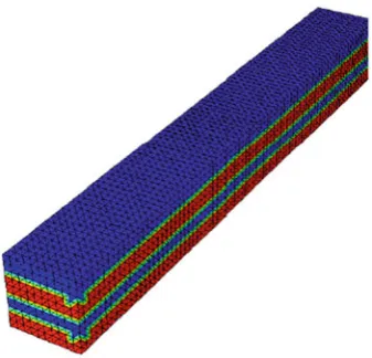
For both three-dimensional scalability test (Sects.5.1and5.2), we use the domain

Fig. 2 Partition ofΩinto L=8 subdomains—regular (left) and Metis (right)

Fig. 3 Coefficient distribution

(four alternating layers)

5.1 The Darcy equation

On the domainΩ ⊂R3given above, we solve the following problem: Findv∈ H1(Ω)

such that

− ∇ ·(κ∇v)=0 in Ω, (5.1)

v =0 on∂ΩD = {(x,y,z)∈∂Ω : x =0}andκ∇v·n =0 on the rest of∂Ω, where n is the outward unit normal. The coefficient distribution alternates between two different constant valuesκ1 andκ2of κ on four horizontal layers (as shown in

Fig.3).

sub-Table 1 3D Darcy: number of PCG iterations (it), condition number (cond) and coarse space dimension

(dim) vs. jump inκforκ1=1,=1 added layers, L=8 regular subdomains

κ2 AS ZEM GenEO

it cond it cond dim it cond dim

1 16 229 11 6.3 8 11 8.4 7

102 27 230 19 22 8 13 8.4 14

104 29 230 23 210 8 15 8.4 14

106 26 230 22 230 8 11 8.4 14

domain is then extended by=1 layers in order to create the overlapping partition. Table1shows the iteration counts and condition numbers for fixed valueκ1=1 and

variousκ2. As expected, for our algorithm the condition number and the number of

PCG iterations are robust with respect to the jumpκ2/κ1. Furthermore, forκ2=κ1,

the algorithm automatically selects seven eigenmodes (one per floating subdomain) to build the coarse space, this leads essentially to the same choice as for the ZEM method except for the subdomain in which the Dirichlet boundary condition is active, where GenEO does not select any coarse mode. In both cases 11 iterations are needed to reach convergence.

The second test that we conduct is the scalability with regard to the problem size and the number of subdomains. For simplicity, we make the problem parameter L vary. Recall that increasing L elongates the bar-shaped domain and at the same time increases the number of subdomains which equals L. Thus, the global number of degrees of freedom is also proportional to L. Table2gives the results for different problem sizes (we display the number of subdomains and the total number of degrees of freedom) and for regular and irregular partitions. For regular partitions we use (3.9); for irregular partitions, the choice of mj becomes more tricky since there may be additional ’bad’ eigenmodes close to the ratioδj/Hjthat are due to the irregularity of the subdomains and not due to any coefficient variation. In particular, the ratioδj/Hj which is constant for regular partitions, as L gets increased, may differ significantly for two ‘Metis’ decompositions into L and Lsubdomains with L =L. In the regular case, (3.9) leads to mj =2 andλ3=0.5. Thus, in order for the bound on the condition

number given by Theorem3.22to be at least as strict in the irregular (’Metis’) case we set

mj := min

#

m:λ_mj₊₁>0.5

$

, (5.2)

in each subdomain in Table2. We note that the condition numbers in both the regular and irregular subdomain cases are stable and consistently low.

Table 2 3D Darcy: number of PCG iterations (it), condition number (cond) and coarse space dimension

(dim) vs. problem size forκ1=1,κ2=106,=1 added layers, L (sub) subdomains

sub glob DOF AS ZEM GenEO

it cond it cond dim it cond dim Regular

4 4,840 14 51 15 51 4 10 8.4 6

8 9,680 26 230 22 230 8 11 8.4 14

16 19,360 51 980 36 970 16 13 8.4 30

32 38,720 103 4,000 61 3,900 32 13 8.4 62

Metis with criterion given by (5.2)

4 4,840 21 67 18 63 4 9 3.0 19

8 9,680 36 290 29 280 8 9 3.0 40

16 19,360 65 1,200 45 1,200 16 11 3.1 81

32 38,720 123 4,900 79 4,700 32 11 3.1 171

Table 3 3D Darcy: number of PCG iterations (it), condition number (cond) and coarse space dimension

(dim) vs. numberof layers added to each domain, for L=8 regular subdomains,κ1=1 andκ2=106

AS ZEM GenEO

it cond it cond dim it cond dim

1 26 230 22 230 8 11 8.4 14

2 22 150 18 150 8 9 5.4 14

3 16 110 15 110 8 9 4.0 14

4 15 92 13 92 8 7 3.3 14

5.2 The linear elasticity equations

For the second family of tests the equations are the following. Find u=(u1,u2,u3)T∈

H1(Ω)3such that

−div(σ(u))=f, inΩ,

u=(0,0,0)Ton∂ΩD = {(x,y,z)∈∂Ω : x =0}andσ (u)·n=0 on the rest of

∂Ω, where the stress tensorσ (u), the Lamé coefficientsλandμand the right hand side are given by

%

σi j(u)=2μεi j(u)+λδi jdiv(u), εi j(u)= 1₂

∂ui ∂xj +

∂uj ∂xi

,f=(0,0,g)T,

μ= E

2(1+ν), λ=

Eν (1+ν)(1−2ν).

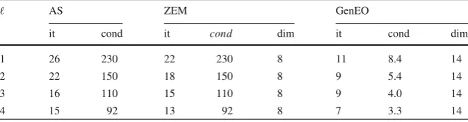
Table 4 3D Elasticity: number of PCG iterations (it), condition number (cond), and coarse space dimension

(dim) vs. number of regular subdomains, for=1 added layers, g=10,(E1, ν1)=(2×1011,0.3)and

(E2, ν2)=(2×107,0.45)

L glob DOF AS ZEM GenEO

it cond it cond dim it cond dim

4 14,520 79 2.4×103 54 2.9×102 24 16 10 46

8 29,040 177 1.3×104 87 1.0×103 48 16 10 102 16 58,080 378 1.5×105 145 1.4×103 96 16 10 214

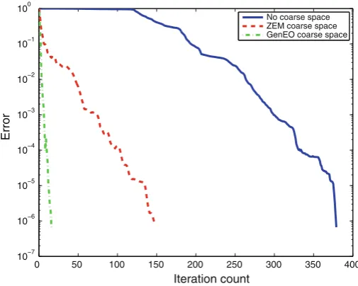
0 50 100 150 200 250 300 350 400

10−7 10−6 10−5 10−4 10−3 10−2 10−1 100

Iteration count

Error

No coarse space ZEM coarse space GenEO coarse space

Fig. 4 3D Elasticity: Relative error vs. iteration count for L=16 regular subdomains

in Fig. 3. Table 4 displays iteration counts, condition numbers, and coarse space dimensions for various partitions into regular subdomains (the parameter choices are given below the table). Note that for GenEO, we need only 16 PCG iterations in all cases. As an example, Fig.4shows the convergence profile for the case whereΩ is split into 16 regular subdomains.

5.3 The two-dimensional linear elasticity equations

IsoValue -1.05053e+10 5.28263e+09 1.58079e+10 2.63332e+10 3.68584e+10 4.73837e+10 5.79089e+10 6.84342e+10 7.89595e+10 8.94847e+10

1.0001e+11

1.10535e+11

1.21061e+11 1.31586e+11

1.42111e+11 1.52636e+11

1.63162e+11

1.73687e+11 1.84212e+11

2.10525e+11

E

Fig. 5 2D Elasticity: coefficient distribution (left)—Metis decomposition into 64 subdomains (right)

Table 5 2D Elasticity: number of PCG iterations (it) and coarse space dimension (dim) vs. number of

Metis subdomains for fixed problem size

sub glob DOF AS ZEM GenEO

it it dim it dim

4 13,122 90 94 12 36 36

16 13,122 169 179 48 39 112

25 13,122 222 157 75 40 166

64 13,122 317 196 192 39 343

on the two regions (indicated by the two different colors) we take the parameters

(E1, ν1)=(2×1011,0.3)and(E2, ν2)=(2×107,0.45).

This time, we keep the problem size fixed, but we make the number of subdo-mains vary. In all cases, we use a Metis partition and extend the non-overlapping subdomains by=2 layers. As shown in Fig.5(right) for a decomposition into 64 subdomains there are many floating subdomains. Table5shows the iteration counts and coarse space dimensions for different Metis partitions (the chosen parameters are given below the table). From the iteration counts we see that the GenEO method is scalable.