Theses Thesis/Dissertation Collections
11-16-2010
Laplacian eigenmaps manifold learning and
anomaly detection methods for spectral images
Marcela Munoz RealesFollow this and additional works at:http://scholarworks.rit.edu/theses
This Thesis is brought to you for free and open access by the Thesis/Dissertation Collections at RIT Scholar Works. It has been accepted for inclusion in Theses by an authorized administrator of RIT Scholar Works. For more information, please [email protected].
Recommended Citation
Laplacian Eigenmaps Manifold Learning
and Anomaly Detection Methods for
Spectral Images
by
Marcela Munoz Reales
A Thesis Submitted in Partial Fulfillment of the Requirements for the Degree of Master of Science
in Applied and Computational Mathematics
Supervised by
Professor Dr. William Basener School of Mathematical Sciences
College of Science
Rochester Institute of Technology Rochester, New York
November 16, 2010
Approved by:
Dr. William Basener, Professor
Thesis Advisor, School of Mathematical Sciences
Dr. David Messinger, Associate Professor
Dr. Bernard Brooks, Associate Professor
Committee Member, School of Mathematical Sciences
Dr. Anthony Harkin, Associate Professor
Rochester Institute of Technology College of Science
Title:
Laplacian Eigenmaps Manifold Learning and Anomaly Detection Methods for Spectral Images
I, Marcela Munoz Reales, hereby grant permission to the Wallace Memorial
Library to reproduce my thesis in whole or part.
Marcela Munoz Reales
Abstract
Laplacian Eigenmaps Manifold Learning and Anomaly Detection Methods for Spectral Images
Marcela Munoz Reales
Supervising Professor: Dr. William Basener
Spectral images provide a large amount of spectral information about a scene,
but sometimes when studying images, we are interested in specific components.
It is a difficult problem to separate the relevant information or what we call
in-teresting from the background of a spectral image, even more so if our target
objects are unknown. Anomaly detection is a process by which algorithms are
designed to separate the anomalous (different) points from the background of
an image. The data is complex and lives in a high dimension, manifold
learn-ing algorithms are used to analyze data that lives in a high dimensional space,
but that can be represented as a lower dimensional manifold embedded in the
high dimensional space. Laplacian Eigenmaps is a manifold learning algorithm
that applies spectral graph theory methods to perform a non-linear
approach to reduce the dimension of the data and separate anomalous pixels in
Contents
Abstract . . . iv
1 Introduction . . . 1
2 Imaging Processing . . . 3
2.1 Classification . . . 6
2.2 Anomaly Detection . . . 7
2.3 Target Detection . . . 8
3 Graph Theory . . . 9
3.1 Example . . . 9
4 Algorithms for Anomaly Detection . . . 11
4.1 PCA . . . 11
4.2 RX . . . 12
4.3 TAD . . . 13
5 Manifold Learning Algorithms . . . 15
5.1 Isomap . . . 17
5.2 Locally Linear Embedding . . . 17
5.3 Laplacian Eigenmaps . . . 18
6 Images . . . 19
7.1 Definitions . . . 24
7.2 Properties of the Laplacian . . . 25
7.3 Algorithm . . . 28
7.4 Output . . . 31
7.5 Social Network with Anomaly example . . . 33
7.5.1 Results . . . 34
8 Laplacian Eigenmaps for Anomaly Detection in Spectral Images Experiments . . . 36
8.1 Example: Simple Chip, Simple Chip with Anomaly . . . 38
8.1.1 Results . . . 39
8.2 Simple Chip with 3 Anomalies . . . 45
8.2.1 Results . . . 45
8.3 Laplacian Anomaly Image . . . 49
8.3.1 Results . . . 50
9 Conclusions . . . 55
10 Future Work . . . 57
A PRO GraphSpectracircle . . . 59
A laplacianprojection.pro . . . 65
List of Figures
2.1 Data cube structure. The figure shows the spectral cube for an
image (middle), a view as a set of spectra per each pixel (left),
or as a single image for each single spectral channel (right)[1] . 4
6.1 Spectral response of WorldView2 panchromatic and
multispec-tral imager . . . 20
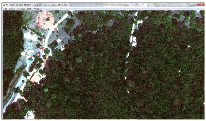
6.2 World View 2 Image . . . 20
7.1 Social Network with anomaly results . . . 34
8.1 Simple Chip and spectral profile for two pixels . . . 38
8.2 Simple Chip with Anomaly and spectral profile for anomalous pixel . . . 39
8.3 Spectrum of the graph for the Simple Chip 8.1, and Simple Chip with Anomaly 8.2 . . . 40
8.4 Left, projection of the spectra of the pixels on spectral bands 1 (blue) and 4 (red). Right, projection onto eigenvectors 0 and 1 of the Laplacian for Simple Chip 8.1 . . . 41
8.5 Left, projection of the spectra of the pixels on spectral bands 1 (blue) and 4 (red). Right, projection onto eigenvectors 0 and 1 of the Laplacian for Simple Chip with Anomaly 8.2 . . . 42
8.7 Left, grayscale projection results for Simple Chip with Anomaly
eigenvector 1. Right, Eigenvector Profiles for the anomaly and
the pixel next to it . . . 44
8.8 Simple Chip with 3 Anomalies . . . 45
8.9 Spectrum of Simple Chip with 1 anomaly vs. Spectrum of
Sim-ple Chip with 3 Anomalies . . . 46
8.10 Left, projection of the spectra of the pixels on spectral bands 1
(blue) and 4 (red). Right,projection onto eigenvectors 0 and 1
of the Laplacian for Simple Chip with 3 Anomalies 8.8 . . . 47
8.11 Left, grayscale projection results for Simple Chip with 3
Anoma-lies eigenvector 1. Right, Eigenvector Profile for background
pixel . . . 47
8.12 Left, grayscale projection results for Simple Chip with Anomaly
eigenvector 1. Right, Eigenvector Profiles for the anomaly and
the pixel next to it . . . 48
8.13 WorldView-2 image, Laplacian Anomaly Image 50x50 Chip
lo-cation shown on red box . . . 49
8.14 Laplacian Anomaly Image- 50x50 Chip . . . 50
8.15 Left, projection of the spectra of the pixels on spectral bands 1
(blue) and 4 (red). Right,projection onto eigenvectors 0 and 1
of the Laplacian for Laplacian Anomaly Image 8.14 . . . 51
8.16 Left, grayscale projection results for Laplacian Anomaly Image
eigenvector 1. Right, Eigenvector Profile for 3 background pixels 52
8.17 Left, grayscale projection results for Laplacian Anomaly Image
eigenvector 1. Right, Eigenvector Profiles for the anomalous
(different) pixels . . . 53
8.18 n-d visualizer for bands 1,2,3, and a selected class (red) that
includes the most distant points (left). Projection of the results
Chapter 1
Introduction
Spectral images are digital images that contain measurements of wavelengths
of light so that a spectrum is provided for each pixel instead of the usual red,
green and blue. They contain complex high dimensional data that is difficult to
study in its original form. Imaging processing methods are used in the study
of the information provided by spectral images. The three most important uses
of image processing are clustering and classification, anomaly detection, and
target detection. We are interested in the problem of anomaly detection.
There are several mathematical tools that can be used to extract information
from spectral data. Statistical models using principal component analysis (PCA)
and Reed-Xiaoli anomaly detector can be applied to analyze the background
in-formation and create a ranking of anomalous pixels in spectral images. PCA is a
by embedding the data into a linear subspace. RX (Reed-Xiaoli anomaly
de-tector) is the most popular anomaly detection algorithm, it uses the covariance
matrix and the distance to the mean to locate anomalies. Spectral graph theory
methods can be used to study spectra variations, and detect anomalies; images
can be modeled as sets of connected components where pixels are vertices with
edges connecting them under specific conditions. TAD (Topological Anomaly
Detection algorithm) creates a graph using the pixel’s spectra as vertices that
are connected if they are spectrally similar.
Manifold learning algorithms are used to analyze data that lives in a high
dimensional space, but that can be represented as a lower dimensional manifold
embedded in the high dimensional space. Laplacian Eigenmaps is a manifold
learning algorithm that uses spectral graph theory concepts to represent spectral
data as a graph, using the pixels’ spectra as vertices that are connected if their
spectra are similar; one can construct a Laplacian matrix from the degree of the
vertices and perform an eigen-decomposition to aid in the search for pixels that
have anomalous spectra.
We present an approach that uses a Laplacian Eigenmaps algorithm for anomaly
Chapter 2
Imaging Processing
Remote sensing tools were designed to capture information about objects
with-out coming into direct contact with them. Remote sensing instruments can be
used in many applications such as to help in the study of crops, characterization
of soils, and mineral exploration [1].
Multi-spectral images are a type of image used in remote sensing. They can
provide information undetectable by the human eye, capturing images in four
or more wavelengths of light, and stored in a file with one band for each
wave-length. As remote sensing progressed, hyperspectral imagery was introduced.
Hyperspectral images have many narrow bands that provide data from across
the electromagnetic spectrum. Each pixel of the image contains many spectral
bands that allow material identification.
Materials have a reflectance spectrum that characterizes them; this is called
would remain unchanged under changing circumstances. But in reality, the
re-flectance spectrum of most materials exhibits variability caused by errors in the
sensor, atmospheric and environmental changes, and variation in the amount
of light absorbed or reflected by the material [2]. It is also worth noting that
man-made material show less spectral variability than objects of the natural
[image:14.612.102.503.284.405.2]en-vironment such as grass, soil, etc.
Figure 2.1: Data cube structure. The figure shows the spectral cube for an image (middle), a view as a set of spectra per each pixel (left), or as a single image for each single spectral channel (right)[1]
Spectral data generated by spectral imagery contains three-dimensional
spatial-spatial-spectral measurements, which can be visualized with what is called the
spectral cube [1]. The x and y (spatial) dimensions of the data cube for each
pixel are the two-dimensional image that the human eye can see, the z
dimen-sion contains spectral information captured by the few hundred bands of the
information comes from the spectral data.
The three most important uses of image processing are:
unmixing/clustering/classification, anomaly detection, and target detection.
Spec-tral unmixing and classification algorithms seek to separate each pixel’s
spec-trum by identifying the endmember spectra for the image and their proportion
in the pixel [3]. Anomaly detection aims to separate the anomalous points from
the background of an image. Target detection is similar to anomaly detection
but with the difference that the objects of interest have known characteristics.
Two desirable characteristics of target and anomaly detection algorithms, other
than being computationally efficient, are high probability of detection and, low
probability of false alarm (low false-alarm-rate).
The first approach of many imaging process algorithms is dimension
reduc-tion. The objective of dimension reduction is to represent the signal in a
mini-mal way that saves the necessary information to perform a successful unmixing
2.1
Classification
Classification is the process of identifying the largest components of the image,
and organizing the pixels according to the endmember component they belong
to.
The spectrum of a mixed pixel contains a mixture of materials, either as a
result of low spatial resolution, or a pixel that is composed of a homogeneous
mixture of materials. Spectral unmixing yields the endmembers and the
pro-portion of each in the pixel, this can be used for clustering and classification.
Endmembers are natural or man-made materials that are part of the image, for
example, grass, water, or different types of concrete [3]. The largest endmember
components of the image can be classified, since they are part of the majority
of pixels, and interpretation of the scene can be done by analyzing the clusters
2.2
Anomaly Detection
Anomaly detection is the process of identifying pixels in an image whose
spec-tra is very dissimilar from the specspec-tra of the background of the image. Anomaly
detection algorithms look for a small number of objects in a scene, for this
rea-son, classification methods are not typically used, because most of the time the
image provides little information about objects of interest or they are not clearly
resolved [1]. In other words, large components of the image are only used in
anomaly detection algorithms as a point of reference to identify anomalous
pix-els.
Anomaly Detection can be more effective when comparing a pixel in an
im-age to its immediate vicinity. One of the most important uses is to recognize
man-made structures or objects from natural surroundings, a car or a house in
the middle of the forest. It can also be used to increase the probability of
2.3
Target Detection
Target detection is the process of identifying pixels in an image whose spectra
matches a known target spectrum or nature. General applications try to identify
small groups of objects with known shape or spectrum in an image. Target
de-tection is widely used for agricultural applications to look for crop infestation.
It can also be used in conjunction with anomaly detection, this is done, by
ex-tracting a set of materials that are anomalous or different, and then verify if the
Chapter 3
Graph Theory
Definitions from [4].
Definition 1. A simple graphGis a finite nonempty set of objects calledvertices
denoted by V(G), together with a set of unordered pairs of distinct vertices of
Gcalled edgesdenoted by E(G).
Definition 2. The degree of a vertex v in a graph G is the number of edges of
Gincident withv, denoted bydv.
Definition 3. A graphGis connected if and only if there exists a path between every pair of verticesu andv in G. Otherwise the graph is disconnected.
Definition 4. A component of a graph G is a subgraph induced by the vertices
of G.
3.1
Example
Consider the following graph Gdefine by vertex and edge sets
G:
a b
c
d
e f
g
Gis disconnected with 2 components.
We can list the degree values for the vertices ofGin a degree table as follows,
Vertex a b c d e f g
Chapter 4
Algorithms for Anomaly Detection
4.1
PCA
Principal Component Analysis (PCA) is a linear dimensionality reduction method;
its approach is to embed high dimensional data into a linear subspace while
pre-serving the most variance in the data possible. It does an orthogonal linear
trans-formation in which the variance of the data is maximal. PCA provides a linear
mapping onto the d principal eigenvectors of the covariance matrix, which is
solved by the dprincipal eigenvalues λ. The low dimensional representation is
4.2
RX
The Reed-Xiaoli anomaly detector commonly known as RX or RXD is a
popu-lar anomaly detection algorithm. It searches for objects in the minor
eigenval-ues. Using every pixel of the image, the meanµand the covariance matrixΓare
computed, and the Mahalanobis distance from the mean to each pixel are used
to detect anomalies. For a test pixelx using the RX algorithm we get:
RX(x) = (x−µ)Γ−1(x−µ)
Which is equal to the number of standard deviations away from the mean of the
data as a multivariate normal distribution [6]
Local RX anomaly detection algorithm compares anomalous pixels to their
immediate vicinity’s background rather than the entire image. This is achieved
by a dual window with a smaller window within a larger outer one, and
com-puting the mean and covariance using the pixels in the larger window, the pixels
in the smaller one are not included in the computation [6].
In Envi, the ENVI RX Anomaly Detection Tool uses the RX algorithm to find
pixels are brighter than the background pixels.
4.3
TAD
Messinger, Basener and Ientilucci proposed an anomaly detection algorithm for
spectral imagery called Topological Anomaly Detection (TAD). Their approach
is to treat the spectral data in their k-dimensional space; without doing a
dimen-sion reduction. The topology of the data is analyzed and points are separated
into background and anomalies. TAD uses combinatorial topology which refers
to studying the structure of the non-parametric space where the objects of
inter-est live using combinatorial methods.
The algorithm creates a graph using a subset of the image’s pixels spectra
with data points x1, x2, ..., xn from the spectral image as the vertices, adding
an edge from xi to xj if pixel xi is spectrally similar to xj. A subset is used
for computational efficiency. The large component of the graph is assumed to
be the background, and smaller components that contain small percentages of
the pixels in the image are ranked according to their distance to the background
Compared to other statistical methods, TAD has the advantage that
measure-ments are taken by calculating the distances between neighboring data points,
instead of the distance to the mean of the total data, which aids in the successful
Chapter 5
Manifold Learning Algorithms
Complex data sets are hard to study in their original form. Manifold
Learn-ing algorithms were developed to analyze data that lives in a high dimensional
space, with the belief that the data can be represented in a lower dimensional
manifold of dimensionalityd, embedded in a high dimensional space of
dimen-sionalityD, such that d < D[7]
.
Definitions from [7]
Definition 5. A homeomorphism is a continuous function whose inverse is also
a continuous function.
Definition 6. A d-dimensional manifold M is a set that is locally homeomorphic
with Rd. For each x ∈ M, there is an open neighborhood around x, Nx, and
a homeomorphism f : Nx → Rd. The neighborhoods are denoted coordinate
patches, and the map is denoted a coordinate chart. The image of the coordinate charts is called the parameter space.
Definition 7. A manifold is considered a smooth (differentiable) manifold, if
An embedding of a manifold M into Rd is a smooth (differentiable)
5.1
Isomap
Isometric feature mapping (Isomap) [7] is a well-known manifold learning
al-gorithm. Its approach is to find the geodesic distances between neighboring data
points using shortest-path distances. Then it uses the Multidimensional Scaling
(MDS) method, which given a matrix of dissimilarity D ∈ Rn×nconstructs a
set of points such that their Euclidean distances match the ones in D, to find
points in a low-dimensional Euclidean space that match the nearest neighbors
geodesic distances found in the first step.
Isomap is a good method to study large data sets, since it gives an estimate
of the dimensionality of the underlying manifold.
5.2
Locally Linear Embedding
LLE [7] is another manifold learning algorithm that was introduced around the
same time as Isomap. The scheme of LLE is to think about a manifold as a
col-lection of coordinate patches that overlap. With a manifold that is sufficiently
linear. By finding the linear patches and describing their geometry, one can find
a mapping to Rd that preserves their geometry and is almost linear.
5.3
Laplacian Eigenmaps
Laplacian Eigenmaps [7] is a manifold learning algorithm that makes use of
spectral graph theory to represent the data as a graph, with nodes connected
by edges if they are near or of similar nature. It uses an approximation to the
manifold structure by the adjacency matrix computed from the data points and
their distances in the manifold. A weighted Laplacian matrix is created from the
adjacency matrix, with weights given by the heat kernel of the Laplace Beltrami
operator in the heat equation. By doing an eigenvalue decomposition, one can
obtain a vast amount of information about the underlying structure, including
geometric characterization of the data.
Belkin and Niyogi showed than in some instances, the results obtained by
the Laplacian Eigenmaps algorithm are equivalent to those obtained by the LLE
Chapter 6
Images
The images we used were taken with a WorldView-2 satellite. WorldView-2
is the first high-resolution 8-band multispectral commercial satellite. It also
contains a high-resolution panchromatic band. The first four primary bands are
blue, green, red, and near-infrared bands. The additional bands are red edge for
better accuracy on vegetation, coastal band for water color studies, yellow band,
and an additional longer wavelength near infrared band. It operates at an altitude
of 770 Km, with a 46 cm panchromatic resolution and 1.84 mt multispectral
Figure 6.1: Spectral response of WorldView2 panchromatic and multispectral imager [9]
[image:30.612.77.474.388.621.2]Chapter 7
Laplacian Eigenmaps
Laplacian Eigenmaps is a dimension reduction algorithm similar to PCA, but
using graph theory methods instead of statistics.
A spectral image is composed of pixels with n spectral bands. We can take
each pixel and treat it as a point in a n-dimensional space, wherenis the number
of bands. We believe that much of the data of interest lives in a lower dimension,
and this the motivation to use Laplacian Eigenmaps.
In their 2002 paper Belkin and Niyogi proposed an approach to obtain and
represent low dimensional data embedded in a high dimensional space. Their
method uses the relationship of the graph Laplacian, the Laplace Beltrami
op-erator on the manifold, and the connections to the heat equation [8]. The
advan-tage of this algorithm is that it is computationally efficient and utilizes
neigh-borhood information, which makes it a good candidate to assist in the problem
pixel’s spectrum is similar in the background, and hope that anomalous pixels
would stick far out.
The algorithm applied to spectral imagery data computes a low-dimensional
representation of the image data in which the distances between a pixel and its
knearest neighbors (in spectral space) are minimized. It is possible to construct
a graph from an image by using pixels as vertices, and adding an edge between
two pixels i and j if their spectra are similar, in such a way that there exist an
edge (i, j) in the graph if the Euclidean distance from the spectrum of i to the
spectrum ofj is less than a defined thresholdt.
We then create a Laplacian matrix from the degree of the vertices in the
graph, and use the eigenvalues and corresponding eigenvectors of the Laplacian
matrix to represent the image in a lower dimensional space. This can be used to
search for anomalies in the network, since the spectrum of an anomalous pixel
should be significantly different from that of its neighbors.
There is an idea derived from perturbation theory [10], that suggests that in
the optimal case the first (smallest) eigenvectors of the Laplacian are indicator
vectors, so that the entry is zero if the vertex is not in the group. In real-life
and reflect minimal changes that help to separate the graph into different
com-ponents. This idea could be of assistance in the analyzes of results for Laplacian
7.1
Definitions
Definition 8. The identity matrixI onnvertices is defined by:
I(i, j) = (
1 ifi =j,
0 otherwise.
Definition 9. The degree matrix D is a diagonal matrix with the (j, j)th entry having valuedj.
Definition 10. The adjacency matrix W for a given graphGis defined by:
W(i, j) = (
1 ifi andj are adjacent,
0 otherwise.
Definition 11. The Laplacian matrix Lfor a simple graph Gis defined by:
L = D −W
Definitions from [11]:
Definition 12. The normalized Laplacian of Gis defined by the matrix
L(i, j) =
1 ifi = j and dv 6= 0, −1
√ didi
ifi andj are adjacent,
0 otherwise.
given by
L = D−1/2
LD−1/2
Which is equivalent to [10]
L = I −D−1/2W D−1/2
part motivated by several sources such as ([11, 12]) that agree that through
empirical studies the normalized Laplacian best capture the underlying graph’s
spectral geometry, and because it contains information about a random walk
used in stochastic processes.
The use of the normalized Laplacian was intuitive as well because for highly
connected nodes,
L(u, v) = p−1
didj
is very small, whereas for poorly connected nodes it is considerably larger.
Since the objective is to identify anomalous pixels whose spectra is very
dif-ferent from the rest of the pixels in the image, when doing the eigenvalue
de-composition the results obtained for the anomalies that we want to detect stick
out from the rest.
7.2
Properties of the Laplacian
The matrixL as defined in 7.1 has the following properties from [10]:
2. ∀f ∈ RNfTLf = 1 2
P
i,jWi,j(fi−fj)
2
3. L is a positive-semidefinite matrix
4. All eigenvalues of Lare positive and real. This results from property 3.
5. An eigenvalue that is equal to 0 indicates that the graph is connected. The
number of connected components of the graph is equal to the number of
eigenvalues that are equal to 0.
These properties are equivalent forL,
Property 1, Lis symmetric because L is symmetric. Multiplying both sides by
the same diagonal matrix results in a symmetric matrix, thereforeD−1/2
LD−1/2
is symmetric.
Property 2 is as follows:
∀f ∈ RNfTLf = 1 2
X
i,j
Wi,j √fi
di −
fj p
Proof
1 2
X
i,j
Wi,j fi
di −
fj p dj !2 = 1 2 X i,j
Wi,j f
2
i
di − 2√fi
di fj p dj + f 2 j dj ! (7.1) = X i f2 i − X i,j
Wi,j(√fi di
fj p
dj
) (7.2)
= fTf −fTD−1/2
W D−1/2
f (7.3)
= fT I −D−1/2W D−1/2f (7.4)
= fTLf (7.5)
2
Property 3, L is positive-semidefinite, such that ∀x ∈ RNxTLx ≥ 0.
Fol-lows from Property 2.
Property 4 follows fromLbeing positive-semidefinite. Refer to [10] for a proof
7.3
Algorithm
1. Read in the image file
LetX be an×barray that contains the spectra of thenpixels in the image,
wherebis the number of bands in the image.
2. Distance matrix
Compute the Euclidean distances. LetS be the distance matrix ofGwhere
the i, jth entry corresponds to the Euclidean distance from the spectra of
pixelito the spectra of pixel j.
3. Construct the graph
Define a threshold t such that t ∈ R+
. Let G be graph with vertex set
V(X) = x1, x2, ..., xn, together with edge setE(X)and ifiandj ∈V(X),
then(i, j)is an edge in Gif and only ifS(i, j) ≤ t.
4. Adjacency matrix
Create an adjacency matrix W fromG.
5. Compute the normalized Laplacian
G[11], first consider the matrixL of the form,
L(i, j) =
dj ifi = j,
−1 ifi andj are adjacent,
0 otherwise.
Compute the degrees of the vertices fromW.
The Laplacian L is of the form defined by 7.1. It can be computed as
follows:
L = D−1/2LD−1/2
6. Spectrum of the graph
Perform an eigen-decomposition onL, to obtain eigenvalues0 ≤ λ1, λ2, ..., λn,
this is the spectrum of graphG(X), and corresponding eigenvectorsφ1, φ2, ..., φn.
Let A be a n×n square matrix whose columns correspond to the
eigen-vectors φ1, φ2, ..., φn. And, let Λ be the diagonal matrix with diagonal
elements λ1, λ2, ..., λn. Acan be factored as,
7. Output results to an Envi image For each pixel
[i, j, x]
where (i, j) are the location coordinates, and x = φx is the eigenvector
corresponding to that pixel in the following way, for each elementAi,j of
matrixA,
Ai,j →[i−i (mod m)
m , i (mod m), j]
Where [i−i (mod m)
m , i (mod m)] are the location coordinates of the
7.4
Output
If the graph G generated by Laplacian Eigenmaps from imageP is connected,
λ1 = 0 (smallest eigenvalue), and when it is not λ1 > 0. The closer λ1 is to
zero, the stronger connected is the big component of the underlying graph. The
first (smallest) eigenvalues and eigenvectors aid in clustering and classification
of the data, specially λ1 and associated eigenvector φ1 are linked to the main
clusters of the data, and are also associated with the optimal cut of the graph,
also identified as the optimal cluster[13]. The second eigenvalue λ2 quantifies
how well connectedGis [12].
The most relevant information about the structure and connections of the
underlying graph is provided by the first or leading eigenvectors and
corre-sponding eigenvalues. Since these eigenvectors are more resistant to normal
fluctuations in the data (such as shades and small changes in the coloration of
the same component), yet they reflect minimal changes that are important when
the aim is to separate the graph into different components [10]. On the other
hand, eigenvalues are affected by all changes, including those that are irrelevant
we use the information contained in the eigenvectors ofG, and the
correspond-ing eigenvalues for indexcorrespond-ing in ascendcorrespond-ing order.
The output of our Laplacian Eigenmaps algorithm for image P with n
pix-els, is an Envi image of the same size onnbands that represent the eigenvectors
φ1, φ2, , φn corresponding to the eigenvalues λ1, λ2, , λn ordered from smallest
to largest. In other words, the spectrum for each pixel is the eigenvector
corre-sponding to that pixel.
Pixels have different shades of gray on the single band Envi grayscale
pro-jections of the results of Laplacian Eigenmaps, together with the spectrum of
many spectral bands. The values of each spectrum on the output of the program
7.5
Social Network with Anomaly example
We can construct a random social network on n vertices with one anomalous
vertex, and apply Laplacian Eigenmaps algorithm.
We create a simple random network R with 100 people,n= 100, randomly
connected and let one vertex be an anomalous person.
LetR be a simple graph with vertex set
V(R) = [0,1,2, ...,99]
The vertices represent the people in our social network.
Generate2×n edges and connect vertices at random. Resulting in edge set
E(R) that represents the connections among the people in the network.
To create an anomaly we first need to define what an anomaly is in our social
network. An anomaly is an individual that has an abnormal number of
connec-tions to other individuals in the network. We take the last vertex and randomly
connect it ton/2vertices inR. The anomaly in this case is an individual that is
7.5.1 Results
We find the Laplacian of the graph R as defined in Section 7.1. Following the
algorithm in Section 7.3 from step 4 through step 6, we obtained the following
[image:44.612.112.498.202.464.2]results 7.1, refer to the appendix PRO GraphSpectracircle for code.
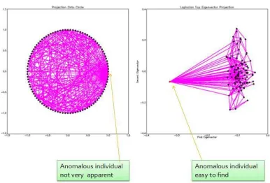
Figure 7.1: Social Network with anomaly results
The figure on the left shows the points forming a circle, with the anomalous
individual shown in red. The figure on the right is the projection of the
indi-viduals onto the plane formed by two eigenvectors, in this case φ1 and φ2, the
x axis ranges from min[φ1] to max[φ1], and the y axis ranges from min[φ2]
coordinates of the eigenvector projected on the 2-dimensional space formed by
φ1 and φ2, nodes for individuals i and j are connected if their corresponding
entry in the adjacency matrixW is 1.
A(i, j) = 1
The anomalous individual sticks out from the rest as expected, having a
signifi-cantly larger number of links to other vertices, and taking values for the first two
eigenvectors that are distant from the rest of the pixels. Whereas the majority
of the pixels are located close to each other in the projection onto the first two
Chapter 8
Laplacian Eigenmaps for Anomaly
Detec-tion in Spectral Images Experiments
For our Laplacian Eigenmaps experiments, we generated several images with
known anomalies. To produce the test images with anomalies, we took some
chips of different sizes from the WorldView-2 image 6.2, and replaced selected
pixels on the images with anomalous pixels. An anomalous pixel is defined as
pixel that comes from a material that does not belong in the test image, and
therefore has a very distinct spectral profile.
We ran the program for the test images and the test images with anomalies.
The thresholdtis set, so after calculating all the Euclidean distances from pixel
ito pixel j in the image, and ranking the distances from smallest to largest, our
algorithm uses the distances that are equal or smaller than the threshold. This
different from the spectra of the rest of the pixels in the image (Euclidean
dis-tance from pixelito pixelj ≥ t) no edges are drawn. For this reason sometimes
we obtain isolated vertices in the graph representation of images, when their
spectra is very disparate, and correspond to anomalous pixels. If an anomalous
object is large and comprises a few pixels in the image, or when working with
larger images it is possible to obtain a separate small component on the graph
8.1
Example: Simple Chip, Simple Chip with Anomaly
• Simple chip:
Is a 10x10 chip of vegetation that is part of WorldView-2 image 6.2 shown
[image:48.612.127.486.275.364.2]in 8 bands, and that exhibits a similar spectral profile for all its pixels.
Figure 8.1: Simple Chip and spectral profile for two pixels
Image 8.1 shows Simple Chip and the spectra of two pixels, note that the
pixels have very similar spectral profiles.
• Simple Chip with Anomaly:
To add an anomaly we started with the Simple Chip of vegetation 8.1, and
replaced the top right corner pixel of the image with a pixel from a
Figure 8.2: Simple Chip with Anomaly and spectral profile for anomalous pixel
Image 8.2 shows Simple Chip with an Anomaly and the spectral profile
of the anomalous pixel, observe how the spectral profile is very different,
with less blue (band 2), and more than double green (band 3), compared to
the spectral profile of the background pixels in Figure 8.1.
8.1.1 Results
For this example, the thresholdtis set at 50 percent.
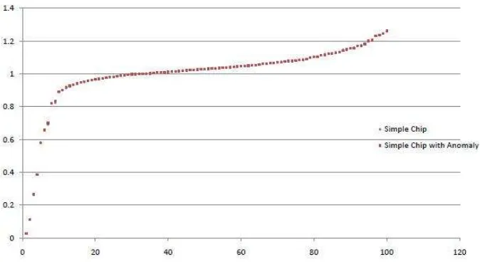
Graph 8.3 shows a plot of the spectrum (eigenvalues) of Simple Chip (in
blue) versus the spectrum of Simple Chip with Anomaly (in red), there is not
much variation on most of the eigenvalues, the major difference is that Simple
Chip with Anomaly has one eigenvalue equal to 1.00, and Simple Chip does
Figure 8.3: Spectrum of the graph for the Simple Chip 8.1, and Simple Chip with Anomaly 8.2
Figure 8.4 shows the projections for the output of the program for Simple
Chip. Left, spectra of the pixels on spectral bands 1(blue) and 4 (red) with
pix-els i and j connected if their corresponding entry in the adjacency matrix A is
1. The projection of the spectra of the pixels on spectral bands 1 and 4 for
Sim-ple Chip shows all the points located close together and connected. Right, the
projection of the pixels onto the plane formed by the first two eigenvectors φ1
andφ2 (IDL starts counting from 0, that is why in the graph we see eigenvectors
0 and 1. In reality we are referring to the first two eigenvectorsφ1 and φ2). The
to max[φ2]. Each node corresponds to a pixel, placed according to the
coordi-nates of the eigenvector projected on the 2-dimensional space formed byφ1 and
φ2, with pixels i and j connected if their corresponding entry in the adjacency
[image:51.612.89.518.198.422.2]matrixW is 1.
Figure 8.4: Left, projection of the spectra of the pixels on spectral bands 1 (blue) and 4 (red). Right, projection onto eigenvectors 0 and 1 of the Laplacian for Simple Chip 8.1
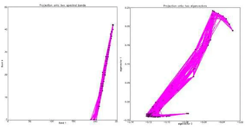
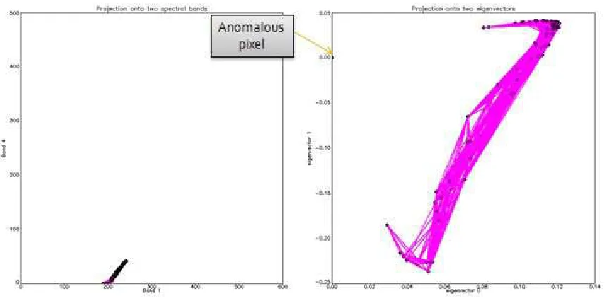
Similarly, Figure 8.5 shows the projections for the output of the algorithm
for Simple Chip.The projection the spectra of the pixels on spectral bands 1 and
4 for Simple Chip with Anomaly shows the anomalous vertex is isolated and
far from the rest of the vertices that are close together and connected. Right,
andφ2, observe how adding a single anomaly alters the projections from Simple
[image:52.612.92.521.129.340.2]Chip 8.4 to Simple Chip with Anomaly 8.5.
Figure 8.5: Left, projection of the spectra of the pixels on spectral bands 1 (blue) and 4 (red). Right, projection onto eigenvectors 0 and 1 of the Laplacian for Simple Chip with Anomaly 8.2
The grayscale projection results for Simple Chip eigenvector 1 are shown on
Figure 8.6 on the images to the left, the Eigenvector Profiles for two pixels are
shown to the right.
The grayscale projection results for Simple Chip with Anomaly eigenvector
1 are shown on Figure 8.7 on the images to the left,the anomalous pixel shows
in white, the Eigenvector Profiles for the anomaly and the pixel next to it are
shown to the right, the anomaly has a zero value for all bands except for a spike
Figure 8.6: Left, grayscale projection results for Simple Chip eigenvector 1. Right, Eigenvector Profiles for two pixels
for all bands.
For this example, Laplacian Eigenmaps shows promising results, it helps to
identify the anomalous pixel. It is interesting that the Eigenvector Profile for
the background pixels takes on values different than zero for most bands
(eigen-vectors) and oscillating within the values 0.3 to -0.3, whereas the Eigenvector
Profile for the anomalous has a zero value for all bands except for a single spike
to 1. This is consistent with the idea mentioned earlier about eigenvectors being
indicator vectors, the anomaly is in one eigenvector only, and is not part of the
8.2
Simple Chip with 3 Anomalies
For this experiment, we started with Simple Chip of vegetation 8.1 used in the
previous section, and replaced three pixels in different parts of the image with
[image:55.612.174.443.224.353.2]pixels from a different image with a very different spectral profile.
Figure 8.8: Simple Chip with 3 Anomalies
8.2.1 Results
For this example, the thresholdtis set at 50 percent.
Graph 8.9 shows a plot of the spectrum of Simple Chip with 1 Anomaly 8.2
(in blue) vs. Spectrum of Simple Chip with 3 Anomalies (in red). There is not
much variation between the two plots, except that there are three eigenvalues
equal to 1.
Figure 8.9: Spectrum of Simple Chip with 1 anomaly vs. Spectrum of Simple Chip with 3 Anomalies
Chip with 3 Anomalies. The spectra of the pixels on spectral bands 1 and 4
(left), and the projection onto the plane formed by the first two eigenvectors,
the anomalous pixels are stacked together on 0 for both eigenvectors.
The grayscale projection results for Simple Chip with 3 Anomalies
eigenvec-tor 1 are shown on Figure 8.11 on the image to the left, the Eigenveceigenvec-tor Profile
for a background pixel is shown to the right.
The grayscale projection results for Simple Chip with 3 Anomalies
Figure 8.10: Left, projection of the spectra of the pixels on spectral bands 1 (blue) and 4 (red). Right,projection onto eigenvectors 0 and 1 of the Laplacian for Simple Chip with 3 Anomalies 8.8
Figure 8.11: Left, grayscale projection results for Simple Chip with 3 Anomalies eigenvector 1. Right, Eigenvector Profile for background pixel
pixels are highlighted, and their Eigenvector Profiles are shown to the left of
every image. Again we see the same behavior as Simple Chip with Anomaly,
the Eigenvector Profiles for the anomalies have a zero value for all bands except
[image:57.612.81.537.362.474.2]22 for the second anomaly (top right), and a spike to 1 in band 24 for the third
anomaly (bottom left). These spikes might be useful in identifying anomalous
[image:58.612.80.530.202.405.2]pixels, anomalies seem consistent here.
8.3
Laplacian Anomaly Image
The Laplacian Anomaly Image is a 50x50 complex chip that is part of
WorldView-2 image 6.WorldView-2. It contains an assortment of materials with different spectral
com-position, such as some vegetation, the ceiling of a building, a road, three cars,
[image:59.612.112.501.251.551.2]among others. Shown on 8.14.
Figure 8.14: Laplacian Anomaly Image- 50x50 Chip
8.3.1 Results
The thresholdtis set at 30 percent for this experiment.
Figure 8.15 shows the projections for the output of the algorithm for
Lapla-cian Anomaly Image. To the left, the projection of the spectra of the pixels on
spectral bands 1 and 4. Right, the projection of the pixels onto the plane formed
by the first two eigenvectorsφ1 andφ2.
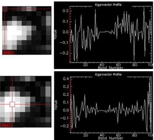
Figure 8.16 shows the grayscale projection results for Laplacian Anomaly
Image eigenvector 1 (left), and Eigenvector Profiles for three background pixels
Figure 8.15: Left, projection of the spectra of the pixels on spectral bands 1 (blue) and 4 (red). Right,projection onto eigenvectors 0 and 1 of the Laplacian for Laplacian Anomaly Image 8.14
of the image shows a lot of variation mainly within values 0.05 and -0.05, and
has values different than zero for almost every single band.
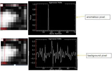
In comparison, figure 8.17 shows the grayscale projection results for Laplacian
Anomaly Image eigenvector 1 (left), and Eigenvector Profiles for the anomalous
or different pixels (right). The spikes or maximum values for the Eigenvector
Profile of anomalies are larger than the values for the background pixels. The
Eigenvector Profiles for those pixels that stick out and that seem to be cars
parked on the road outside the building, have a zero value for the majority bands,
Figure 8.16: Left, grayscale projection results for Laplacian Anomaly Image eigenvector 1. Right, Eigenvector Profile for 3 background pixels
The results of the program visualized in three dimensions for bands
(eigen-vectors) 1, 2, 3 are shown in 8.18 (left), most of the points are close together
with the exception of a few points that are far away from the rest, we selected
these points and created a new class that is shown in red. The image on the right,
shows the grayscale projection for eigenvector 1, the pixels in red correspond to
Figure 8.17: Left, grayscale projection results for Laplacian Anomaly Image eigenvector 1. Right, Eigenvector Profiles for the anomalous (different) pixels
The Laplacian Eigenmaps program successfully identified the anomalous
pixels in the image, as pixels that are far apart from the rest of the pixels, and
Chapter 9
Conclusions
The Laplacian Eigenmaps program successfully identified anomalous pixels in
the experiments performed. By using the information provided by the first
eigenvectors of the Laplacian matrix of the graph constructed from the image,
we were able to find information that could not be easily visualized with the
original data provided by the spectral image.
The anomalies are visually apparent without a great amount of effort on the
Envi projections of the results of the program. And their Eigenvector Profiles
consistently show a similar behavior with zero for most bands and big spikes
in the bands where the anomalous spectrum is present. It is still a question
why these spikes on the spectra of the anomalies happen, but the anomalies
seem show this behavior time and again. We believe it is related to the idea
of eigenvectors being indicator vectors, and point out anomalies that are not
Chapter 10
Future Work
At the moment we are working with 50x50 chips of big images, we would like
to create a procedure to divide the image into multiple tiles and expand our
program to iteratively separate major components of the graph from different or
anomalous components . The next step would be to make Laplacian Eigenmaps
into an anomaly detection algorithm.
The Laplacian Eigenmaps algorithm provides an enormous amount of
infor-mation about the graph used to represent the data that could have other uses in
imaging processing, and not just related to anomaly detection.
Our current algorithm creates a simple graph with no weighted edges, it
would be interesting to assign weights to edges according to how similar the
spectra of the pixels is. This will give us more insight on the structure of the
graph; since it would exploit the heat kernel and aid to find a geometric
the vertices in the manifold vector space, i.e. shortest path between each pair
of vertices in the manifold, which can be used to determine and encapsulate
the structure of the manifold M. This could be useful for classification and
Appendix A
PRO GraphSpectracircle
sample_graph=2
if sample_graph eq 2 then begin ; random graph with anomaly seed=systime(1)
n_vertices = 100;list of vertices V = indgen(n_vertices)
deg = intarr(n_vertices) print, ’vertices: ’ print, V
n_edges=n_vertices*2; list of edges
E = floor((n_vertices-1)*(randomn(seed,2,n_edges,uniform=1))) print, ’E:’
print, E
for i=0,(n_vertices/2-2) do begin
E = transpose([transpose(E),transpose([n_vertices-1,i*2])]) endfor
edge_list = E size_E = size(E) n_edges = size_E[2] print, ’edges: ’ print, E
endif
;Compute degrees of edges and create matrices L and T
L = intarr(n_vertices,n_vertices) Tsqrt = fltarr(n_vertices,n_vertices) for i=0,n_edges-1 do begin
if (E[0,i] NE E[1,i]) then begin L[E[0,i],E[1,i]] = -1
L[E[1,i],E[0,i]] = -1 endif
deg(E[0,i]) = deg(E[0,i])+1 deg(E[1,i]) = deg(E[1,i])+1 endfor
for i=0,n_vertices-1 do begin L[i,i]=deg[i]
Tsqrt[i,i]= 1/sqrt(deg[i]) endfor
print, ’Graph L:’ print, L
print, ’Graph Tˆ(-1/2):’ print, Tsqrt
; Compute the Laplacian Lap=Tsqrt#L#Tsqrt
print, ’Laplacian:’ print, Lap
; Compute the eigenvalues and eigenvectors of the Laplacian A = Lap
TRIRED, A, D, E
; Compute the eigenvalues (returned in vector D) and ; the eigenvectors (returned in the rows of the array A): TRIQL, D, E, A
; Print eigenvalues and eigenvectors
;print, ’
;print, ’Eigenvalues: ’ ;print, D
;print, ’ ’
;print, A[*,0]
if sample_graph eq 3 then begin; for random graph with one anomaly !P.MULTI = [0, 1,3]
window, 0, xsize=400, ysize=600 D_idx = sort(D)
x_range=[min(A[*,D_idx[0]]),max(A[*,D_idx[0]])] x_range=[x_range[0]-(x_range[1]-x_range[0])/10,x_range[1]+ (x_range[1]-x_range[0])/10] y_range=[min(A[*,D_idx[1]]),max(A[*,D_idx[1]])] y_range=[y_range[0]-(y_range[1]-y_range[0])/10,y_range[1]+ (y_range[1]-y_range[0])/10]
plot, A[0:1,D_idx[0]], A[0:1,D_idx[1]], psym=4, symsize=0.5, $ xrange=x_range, yrange=y_range, background=!P.COLOR, color=0, $; set up color and title for plot
thick=2, ymargin=[5,5], charsize=0.5, ticklen=0,$ title=’Laplacian Top Eigenvector Projection’, $ xtitle=’First Eigenvector’, $
ytitle=’Second Eigenvector’ for edge=0,n_edges-1 do begin
nodes = [edge_list[0,edge],edge_list[1,edge]] print, nodes
oplot, A[nodes,D_idx[0]], A[nodes,D_idx[1]], $ psym=0, symsize=0.5, $
thick=2, color=’FF00FF’x endfor
oplot, A[(n_vertices-2):(n_vertices-1),D_idx[0]], A[(n_vertices-2): (n_vertices-1),D_idx[1]], psym=4, symsize=0.5, $
thick=2, color=’0000FF’x
oplot, A[0:(n_vertices-2),D_idx[0]], A[0:(n_vertices-2),D_idx[1]], psym=4, symsize=0.5, $
thick=2, color=0
plot, A[*,D_idx[0]], $
background=!P.COLOR, color=0, $
thick=2, ymargin=[5,5], charsize=0.5, ticklen=0,$ title=’First Eigenvector’
background=!P.COLOR, color=0, $
thick=2, ymargin=[5,5], charsize=0.5, ticklen=0,$ title=’Second Eigenvector’
window, 1, xsize=400, ysize=600 e1 = n_vertices-2
e2 = n_vertices-3 D_idx = sort(D)
x_range=[min(A[*,D_idx[0]]),max(A[*,D_idx[0]])] x_range=[x_range[0]-(x_range[1]-x_range[0])/10,x_range[1]+ (x_range[1]-x_range[0])/10] y_range=[min(A[*,D_idx[1]]),max(A[*,D_idx[1]])] y_range=[y_range[0]-(y_range[1]-y_range[0])/10,y_range[1]+ (y_range[1]-y_range[0])/10]
plot, A[0:1,D_idx[e1]], A[0:1,D_idx[e2]], psym=4, symsize=0.5, $ xrange=x_range, yrange=y_range, background=!P.COLOR,
color=0, $; set up color and title for plot
thick=2, ymargin=[5,5], charsize=0.5, ticklen=0,$ title=’Laplacian Top Eigenvector Projection’, $ xtitle=’First Eigenvector’, $
ytitle=’Second Eigenvector’ for edge=0,n_edges-1 do begin
nodes = [edge_list[0,edge],edge_list[1,edge]] print, nodes
oplot, A[nodes,D_idx[e1]], A[nodes,D_idx[e2]], $ psym=0, symsize=0.5, $
thick=2, color=’FF00FF’x endfor
oplot, A[(n_vertices-2):(n_vertices-1),D_idx[e1]], A[(n_vertices-2): (n_vertices-1),D_idx[e2]], psym=4, symsize=0.5, $
thick=2, color=’0000FF’x
oplot, A[0:(n_vertices-2),D_idx[e1]], A[0:(n_vertices-2), D_idx[e2]], psym=4, symsize=0.5, $
thick=2, color=0 plot, A[*,D_idx[e1]], $
background=!P.COLOR, color=0, $
title=’First Eigenvector’ plot, A[*,D_idx[e2]], $
background=!P.COLOR, color=0, $
thick=2, ymargin=[5,5], charsize=0.5, ticklen=0,$ title=’Second Eigenvector’
endif
if sample_graph eq 2 then begin; for random graph with one anomaly !P.MULTI = [0, 2, 1]
window, 0, xsize=1200, ysize=600
D_idx = sort(D) x_range=[-1.2,1.2] y_range=[-1.2,1.2]
x_coords=cos(indgen(n_vertices)*2*3.141597/n_vertices) y_coords=sin(indgen(n_vertices)*2*3.141597/n_vertices) plot, x_coords[0:1], y_coords[0:1], psym=4, symsize=0.5, $
xrange=x_range, yrange=y_range, background=’FFFFFF’x, color=0, $; set up color and title for plot
thick=2, ymargin=[5,5], charsize=0.5, ticklen=0,$ title=’Projection Onto Circle’
for edge=0,n_edges-1 do begin
nodes = [edge_list[0,edge],edge_list[1,edge]] print, nodes
oplot, x_coords[nodes], y_coords[nodes], $ psym=0, symsize=0.5, $
thick=2, color=’FF00FF’x endfor
oplot, x_coords[(n_vertices-2):(n_vertices-1)], y_coords[(n_vertices-2): (n_vertices-1)], psym=4, symsize=0.5, $
thick=2, color=’0000FF’x
oplot, x_coords[0:(n_vertices-2)], y_coords[0:(n_vertices-2)], psym=4, symsize=0.5, $
thick=2, color=0
D_idx = sort(D)
x_range=[x_range[0]-(x_range[1]-x_range[0])/10,x_range[1]+ (x_range[1]-x_range[0])/10]
y_range=[min(A[*,D_idx[1]]),max(A[*,D_idx[1]])]
y_range=[y_range[0]-(y_range[1]-y_range[0])/10,y_range[1]+ (y_range[1]-y_range[0])/10]
plot, A[0:1,D_idx[0]], A[0:1,D_idx[1]], psym=4, symsize=0.5, $ xrange=x_range, yrange=y_range, background=!P.COLOR, color=0, $; set up color and title for plot
thick=2, ymargin=[5,5], charsize=0.5, ticklen=0,$ title=’Laplacian Top Eigenvector Projection’, $ xtitle=’First Eigenvector’, $
ytitle=’Second Eigenvector’ for edge=0,n_edges-1 do begin
nodes = [edge_list[0,edge],edge_list[1,edge]] print, nodes
oplot, A[nodes,D_idx[0]], A[nodes,D_idx[1]], $ psym=0, symsize=0.5, $
thick=2, color=’FF00FF’x endfor
oplot, A[(n_vertices-2):(n_vertices-1),D_idx[0]], A[(n_vertices-2): (n_vertices-1),D_idx[1]], psym=4, symsize=0.5, $
thick=2, color=’0000FF’x
oplot, A[0:(n_vertices-2),D_idx[0]], A[0:(n_vertices-2), D_idx[1]], psym=4, symsize=0.5, $
thick=2, color=0
endif
Appendix A
laplacianprojection.pro
pro Laplacian_Projection_define_buttons, buttonInfo compile_opt STRICTARR
;compile_opt idl2
envi_define_menu_button, buttonInfo, value=’Laplacian Projection’, $
position=’first’, ref_value=’User Functions’, uvalue=’none’, $
event_pro=’Laplacian_Projection’ end
PRO Laplacian_Projection_doit, fid, dims, plot_distances, plot_eigenvalues
; read in the image
ENVI_FILE_QUERY, fid, fname=fname, nb=nb
; get information from image on the number of bands rows = dims[4]-dims[3]+1
cols = dims[2]-dims[1]+1 bands = nb
Im = fltarr(cols,rows,bands) ; sets up array to hold the image for band=0,nb-1 do begin
Im[*,*,band] = ENVI_GET_DATA(fid=fid, dims=dims, pos=band)
!P.MULTI = 0 ; 1 plot per window
; X is an array that has the spectra of the pixels as columns
; So the spectra of pixel i is X[i,*] X = double(reform(Im, rows*cols,bands))
; List of vertices and vertex information n_vertices = rows*cols
V = indgen(n_vertices) deg = intarr(n_vertices)
;print, ’vertices: ’ ;print, V
; Compute the distance matrix D.
; D[i,j] is the distance from the spectra of pixel i to the spectra of pixel j
Dist = fltarr(n_vertices,n_vertices) for i=0,n_vertices-1 do begin
for j=0,n_vertices-1 do begin Dist[i,j]=norm(X[i,*]-X[j,*]) endfor
endfor
; Sort the distances to find a good threshold threshold_percent= 0.3
S = sort(Dist) Dist_list = Dist[S]
threshold = Dist_list[floor(n_elements(Dist_list)* threshold_percent)]
threshold_line = fltarr(n_elements(Dist_list)) threshold_line[*] = threshold
for i=0,n_vertices-1 do begin Id(i,i) = 1
endfor
Adj = (Dist LE threshold)
; Plot the distances.
if (plot_distances eq 1) then begin window, 0
plot, Dist_list, background=!P.COLOR, color=0 oplot, threshold_line, color=’0000A0’x
endif
; Compute the degrees of the vertices. deg = fix(total(Adj,1))
;print, ’deg’ ;print, deg
; Compute degrees of edges and create matrices L and T
; Actually, we comute Tsqrt=Tˆ(-1/2) which is used to compute ; the Laplacian. Also, we compute L and T at the same to ; avoid looping though vertices multiple times.
L = intarr(n_vertices,n_vertices) Tsqrt = fltarr(n_vertices,n_vertices) I= Identity(n_vertices)
L = I-Adj ;print,’I’ ;print, I ;print,’Adj’ ;print, Adj ;print,’L’ ;print,L
for i=0,n_vertices-1 do begin L[i,i]=deg[i]
Tsqrt[i,i]= -1/sqrt(deg[i]) endfor
;print, ’Graph Tˆ(-1/2):’ ;print, Tsqrt
; Compute the Laplacian Lap=Tsqrt#L#Tsqrt
; print, ’Laplacian:’ ; print, Lap
; Compute the eigenvalues and eigenvectors of the Laplacian A = Lap
TRIRED, A, D, E
; Compute the eigenvalues (returned in vector D) and ; the eigenvectors (returned in the rows of the array A): TRIQL, D, E, A
; Print eigenvalues and eigenvectors ;print, ’
;print, ’Eigenvalues: ’ ;print, D
;print, ’ ’
;print, ’Eigenvectors: (rows of the following array) ’ ;print, A
;print, A[*,0]
;sort the eigenvectors and eigenvales eigen_order = sort(D)
D = D[eigen_order] print, D
print, ’ ’
A_temp = A
for i = 0,n_vertices-1 do begin A[*,i]=A_temp[*,eigen_order[i]] endfor
plot_graph = 1
second_band = 4
first_eigenvector = 1 second_eigenvector = 2 !P.MULTI = [0,2,1]
window, 1, xsize=1200, ysize=600
; plotting nodes on two bands of the image x_range=[0,max(X[*,first_band])]
y_range=[0,max(X[*,second_band])]
plot, X[*,first_band], X[*,second_band], psym=4, symsize=0.5, $
xrange=x_range, yrange=y_range, background=!P.COLOR, color=0, $
; set up color and title for plot
thick=2, ymargin=[5,5], charsize=0.5, ticklen=0,$ title=’Projection onto two spectral bands’, $ xtitle=’Band ’+strtrim(first_band,2), $
ytitle=’Band ’+strtrim(second_band,2) for i=0,n_vertices-1 do begin
for j=0,n_vertices-1 do begin if (Adj[i,j] eq 1) then begin
nodes = [i,j]
oplot, X[nodes,first_band], X[nodes,second_band], $ psym=0, symsize=0.5, $
thick=2, color=’FF00FF’x endif
endfor endfor
oplot, X[*,first_band], X[*,second_band], psym=4, symsize=0.5, color=0
;plotting nodes on the Eigenvectors D_idx = sort(D)
x_range=[min(A[*,D_idx[first_eigenvector]]),max(A[*, D_idx[first_eigenvector]])]
plot, A[*,D_idx[first_eigenvector]], A[*,D_idx[second_eigenvector]], psym=4, symsize=0.5, $
xrange=x_range, yrange=y_range, background=!P.COLOR, color=0,$; set up color and title for plot
thick=2, ymargin=[5,5], charsize=0.5, ticklen=0,$ title=’Projection onto two eigenvectors’, $
xtitle=’eigenvector ’+strtrim(first_eigenvector,2), $ ytitle=’eigenvector ’+strtrim(second_eigenvector,2)
for i=0,n_vertices-1 do begin for j=0,n_vertices-1 do begin
if (Adj[i,j] eq 1) then begin nodes = [i,j
oplot, A[nodes,D_idx[first_eigenvector]], A[nodes,D_idx [second_eigenvector]], $
psym=0, symsize=0.5, $ thick=2, color=’FF00FF’x endif
endfor endfor
oplot, A[*,D_idx[first_eigenvector]], A[*,D_idx[second_eigenvector]], psym=4,
symsize=0.5, color=0 endif
; put image into memory
out_image = reform(A,cols,rows,rows*cols) envi_enter_data, out_image
!P.MULTI = 0 ; 1 plot per window end
pro Laplacian_Projection, ev compile_opt STRICTARR
; compile_opt idl2
; Select input file and get relevant stats
’Select Input File for Laplacian Projection’ if (fid[0] eq -1) then return
base = widget_auto_base(title=’Laplacian Projection Paramters’)
s1 = widget_base(base, /column, /frame) s2 = widget_base(s1, /row)
param6 = widget_menu(s2, /auto, /exclusive,
prompt=’Plot Distances: ’, list=[’No’, ’Yes’], default_ptr=1, uvalue=’plot_distances’)
s2 = widget_base(s1, /row)
param6 = widget_menu(s2, /auto, /exclusive, prompt= ’Plot Eigenvaluess: ’, list=[’No’, ’Yes’], default_ptr=1, uvalue=’plot_eigenvalues’)
res = auto_wid_mng(base)
if (res.accept eq 0) then return plot_distances = res.plot_distances plot_eigenvalues = res.plot_eigenvalues
Laplacian_Projection_doit, fid, dims, plot_distances, plot_eigenvalues
Bibliography
[1] D. Manolakis, D. Marden, and G. Shaw, “Hyperspectral Image Processing
for Automatic Target Detection Applications,” Lincoln Laboratory Volume
14.
[2] G. Shaw and H. Burke, “Spectral Imaging for Remote Sensing,” Lincoln
Laboratory Volume 14.
[3] N. Keshava, “A Survey of Spectral Unmixing Algorithms,” Lincoln
Labo-ratory Volume 14.
[4] G. Chartrand and L.Lesniak, Graphs and Digraphs. New York: Chapman
and Hall, 2005.
[5] L. Maaten, E. Postma, and J. Herik, “Dimensionality Reduction: A
Com-parative Review,” TiCC.
Anomalies in Spectral Imagery, Algorithms and Technologies for
Multi-spectral, HyperMulti-spectral, and Ultraspectral Imagery XV,” SPIE.
[7] L. Cayton, “Algorithms for manifold learning,” UCSD tech report
CS2008-0923, 2005.
[8] M. Belkin and P. Niyogi, “Laplacian Eigenmaps for Dimensionality
Re-duction and Data Representation, Neural Computation,” 15
(6):1373-1396, 2003.
[9] I. DigitalGlobe, “Worldview2 spectral response,” Available at
http://www.digitalglobe.com.
[10] U. Heinemann, “Anomaly Detection in Networks by their Laplacians’
Di-vergence Measures,” School of Computer Science and Engineering. The
Hebrew University of Jerusalem.
[11] F. R. K. Chung, “Spectral Graph Theory,” CBMS Regional Conference
Series in Mathematics. American Mathematical Society, Rhode Island.
[12] R. Johnson and T. Zhang, “On the Effectiveness of Laplacian
Research 8 (2007), pp. 1489–1517, 2007.
[13] S. Kounev, I. Gorton, and K. E. Sachs, “Performance Evaluation: Metrics,
Models and Benchmarks,” SPEC International Performance Evaluation
Workshop, 2008.
[14] F. Roli and S. Vitulano, “Image analysis and processing ,” ICIAP 13th
![Figure 2.1: Data cube structure. The figure shows the spectral cube for an image (middle), aview as a set of spectra per each pixel (left), or as a single image for each single spectral channel(right)[1]](https://thumb-us.123doks.com/thumbv2/123dok_us/54599.5014/14.612.102.503.284.405/figure-structure-gure-spectral-middle-spectra-spectral-channel.webp)