Nonlinear optics and saturation behavior of quantum dot samples under continuous wave driving

Nonlinear optics and saturation behavior of

quantum dot samples under continuous wave

driving

T. Ackemann, A. Tierno, R. Kuszelewicz, S. Barbay, M. Brambilla, C. G. Leburn, and C. T. A. Brown

AbstractThe nonlinear optical response of self-assembled quantum dots is rele-vant to the application of quantum dot based devices in nonlinear optics, all-optical switching, slow light and self-organization. Theoretical investigations are based on numerical simulations of a spatially and spectrally resolved rate equation model, which takes into account the strong coupling of the quantum dots to the carrier reser-voir created by the wetting layer states. The complex dielectric susceptibility of the ground state is obtained. The saturation is shown to follow a behavior in between the one for a dominantly homogeneously and inhomogeneously broadened medium. Approaches to extract the nonlinear refractive index change by fringe shifts in a cav-ity or self-lensing are discussed. Experimental work on saturation characteristic of InGa/GaAs quantum dots close to the telecommunication O-band (1.24-1.28µm) and of InAlAs/GaAlAs quantum dots at 780 nm is described and the first

demonstra-T. Ackemann

SUPA and Department of Physics, University of Strathclyde, Glasgow G4 0NG, Scotland, UK. e-mail: [email protected]

A. Tierno

Universit´e de Nice Sophia Antipolis, Institut Non-Lin´eaire de Nice, UMR 6618, 06560 Valbonne, France. e-mail: [email protected]

R. Kuszelewicz, S. Barbay

Laboratoire de Photonique et de Nanostructures, CNRS, Route de Nozay, 91460 Marcoussis, France. e-mail: [email protected], [email protected]

M. Brambilla

CNISM e Dipartimento Interateneo di Fisica, via Amendola 173, 70126 Bari, Italy. e-mail: [email protected]

C. G. Leburn

SUPA and School of Engineering and Physical Sciences, Heriot-Watt University, Edinburgh EH14 4AS, Scotland, UK. e-mail: [email protected]

C. T. A. Brown

SUPA and School of Physics and Astronomy, University of St. Andrews, St. Andrews, KY16 9SS, Scotland, UK. e-mail: [email protected]

tion of the cw saturation of absorption in room temperature quantum dot samples is discussed in detail.

1 Introduction

As witnessed by the contributions in this book, semiconductor quantum dots (QD) are finding considerable interest for laser, amplifier and quantum information de-vices. The 3D quantum confinement leads to a ‘quasi-atomic’ behavior with a delta function-like density of states resulting, from the applications point of view, in many realized or anticipated benefits such as low threshold currents, low temperature sen-sitivity and low phase-amplitude coupling.

From the fundamental point of view, it seems interesting to revisit linear and nonlinear effects known for atoms – or their archetypical abstraction, the ‘two-level’ atom, in QD ‘artificial’ atoms. In contrast to real atoms, QD size, density and mate-rial composition can be used to tailor emission wavelengths and other characteris-tics. The analogy between QD and atoms was most explored for single dots due to their relevance for quantum information devices, e.g. [1, 2, 3]. Saturation behavior typical for two-level atoms is reported in these Refs. However, in order to take ad-vantage of long dephasing times cryogenic temperatures are required. Moving over to ensembles of QD, but still at cryogenic temperatures, self-induced transparency was demonstrated as a specific phenomenon in nonlinear beam propagation in two-level systems [4], and spectral hole burning in [5] mimicking the corresponding effect in Doppler broadened atomic systems.

At room temperature, work on nonlinear optical properties focused on the gain regime due to the relevance for semiconductor optical amplifiers (SOAs), most often under pulsed excitation [6, 7, 8, 9, 10, 11, 12], but also under cw conditions [6, 9, 13, 14, 15, 16]. In contrast, studies under absorptive conditions seem to be limited either to pulsed excitation [7, 8, 17, 18, 19], motivated by applications as semiconductor saturable absorption mirrors (SESAMs), or to collodial ensembles [20, 21].

condi-tions. Obviously, this enhanced flexibility of QD might be not only beneficial for solitons but for nonlinear optics in general.

Moreover, characterizing the nonlinear index response to external optical driv-ing provides also an alternative approach to the important problem of characterizdriv-ing phase-amplitude coupling in QD. Due to their symmetric, atom-like gain spectrum, ‘ideal’ QD should have zero phase-amplitude coupling or linewidth enhancement factor (orα-factor [34]) at gain maximum and hence a reduced tendency to insta-bilities compared to quantum well and bulk devices. Indeed, a reducedα-factor and a reduced tendency to beam filamentation was observed in many QD samples under some operating conditions [35, 36, 37, 38], but also fairly strong phase-amplitude coupling under different operating conditions [38, 39, 40]. Characterizing nonlinear phase shifts and/or the resulting self-lensing effects would give a direct indication of the tendency of the system to filamentation and help to identify the appropriate oper-ation conditions for applicoper-ations demanding low (lasers, amplifiers, absorptive non-linearities) and high (dispersive optical nonnon-linearities) phase-amplitude coupling.

driv-ing also for these. Sec. 5 provides a brief summary of the issues discussed and an outlook on improving the nonlinear figure of merit of devices.

2 Modeling and simulation results

2.1 The Model

The modeling of semiconductor QD requires a number of assumptions, according to a variety of preconditions: in the first instance, the growth and sample character-istics, as well as the current and/or optical injection conditions. The most appealing feature of QD being their quasi-atomic susceptibility, one aims to have a clear set of discrete states from quantum confinement, the best separated as possible from the carriers states defined in the wetting layer (WL) which is generally considered as a quantum well and the barrier substrate where the carriers are injected via electric contacts. The description of the QD states depends, in turn, on the sample inasmuch as, e.g., Stranski-Krastanow (SK) growth induces an inhomogeneous broadening of the energy dot states, while a submonolayer deposition yields a larger homogeneity of the dot size [36]. In this work, we will consider a system of small and/or shallow confined QD so that either there is only one electron and one hole bound states, or in case other discrete states exists, these are well separated from the inhomogeneously broadened fundamental transition. The InAlAs/AlGaAs QD discussed in Sec. 4 are an example for the latter, whereas in the InAs/GaAs QD discussed in Sec. 3 several excited QD states (ES) roughly equally spaced between WL and GS exist. In our treatment, the carriers in the ES [14, 16] are not explicitly taken into account but it is assumed that WL and excited states constitute a common reservoir for the QD ground state population [13]. Due to the large separation between the lifetimes of the carriers in the QD ground state (100 ps to 2 ns) and the fast coupling between the other states to the ground state (100 fs to some ps) [16, 9] the details of this coupling are not very important for the properties of the cw state, if probing and pumping are done at the same frequency. Hence, we will use ‘QD population’ synonymous to ‘QD ground state population’ and ‘WL layer population’ synonymous to ‘WL and excited QD state population’.

and continuous states is taken into account via the relaxation mechanism between the GS states and the outside world (WL).

In the model we describe the articulate and still partially unclear relaxation mech-anisms of QD ensembles through phenomenological transition and escape/capture rates for intra-dot decays/recombinations and QD-WL carrier relaxations. The spin dynamics is neglected since the spin memory is lost very fast at room temperature [43, 44].

The coupling mechanisms between the WL and the QD considered are the carrier escape and capture by the dot via thermo-activation through emission or absorption of lattice phonons and Auger processes at first order in the WL populations, which include Pauli blocking effects, under the assumption that the sample is passive or weakly pumped [45].

2.1.1 Carrier dynamics and dielectric susceptibility

Following [23], we derive the equations for the expectation values of the number of particles operator for the electrons and holes and for the corresponding polarization

p:

dne,h

dt =−γnrn e,h_−Γ

spnenh+i

¯

h(µp

∗_−µ∗_p)E+dne,h dt

¯ ¯ ¯ ¯

QD−W L

+dne,h

dt ¯ ¯ ¯ ¯ Auger

QD−W L

,

(1)

d p

dt =−(iωa+γp)p− i

¯

h h

ne+nh−1

i

dE, (2)

whereγnris the non radiative recombination rate,Γspthe bimolecular coefficient

for spontaneous recombination, ωa the electron-hole recombination pulsation,γp

the polarization damping, E=Eexp(−iω0t) +c.c. is the electric field andµ the

dipole transition matrix element.

If we consider the level degeneracyΠ =2 for the two opposite spins, we can introduce the QD populationne_QD,h =Πne,h, the total polarization pQD=Πp and

assume a real dipole momentµ. In the rotating wave approximation and introducing

pQD=PQDexp(−iω0t) +c.c., Eqs. (1,2) become dPQD

dt =−γp(i∆+1)PQD− iµE

¯

h h

ne_QD+nh_QD−Πi, (3)

dne_QD,h

dt =−γnrn e,h QD−

Γsp

2 n

e QDnhQD+

iµ ¯

h (EP ∗

QD−E∗PQD)+

∂ne_QD,h

∂t ¯ ¯ ¯ ¯ ¯

QD−W L

+ ∂n

e,h QD ∂t ¯ ¯ ¯ ¯ ¯ Auger

QD−W L

where we have introduced the detuning from a single dot resonance∆= (ωa−

ω0)/γp.

The first QD-WL relaxation term describes the thermo-activated processes. For the sake of simplicity we ignore the possible non local interaction between the QD and the WL, drop the subscript QD in the variable names and write

∂ne,h

∂t ¯ ¯ ¯ ¯

QD−W L

=−γ_esce,hne,h+σ_cape,hN_{W L}e,h h

Π−ne,h i

, (5)

whereN_{W L}e,h is the surface density carrier population in the WL.γesce,handσcape,h are

respectively the escape rate from the QD and the capture rate cross-section into the QD. The second QD-WL relaxation terms describe the Auger processes [45]. For a low WL carrier density, we retain only those terms that are in first order inN_{W L}e,h:

∂ne

∂t ¯ ¯ ¯ ¯ Auger

QD−W L

=−BheNW Lh ne h

Π−nh i

+BehNW Le nh[Π−ne]. (6)

The first term describes the excitation of an electron to the WL via the interaction of a hole in the WL and in the QD, and the second term is a symmetric process that describes the capture of a WL electron in the QD via the interaction of a WL and a QD hole. For the sake of conciseness, we will refer to the symmetric process in the following by “sym.” in the equations.Bhe,eh has the units of a cross-sectional rate

(area/time). A similar term exists for the holes:

∂nh

∂t ¯ ¯ ¯ ¯ Auger

QD−W L

=−∂ne

∂t ¯ ¯ ¯ ¯ Auger

QD−W L

. (7)

The QD polarizationPQDcan be adiabatically eliminated due to the fast

polar-ization decay timeγ−1

p with respect to the other ones so that its steady state values

is:

PQD=−iµ

¯

hγp µ

1−i∆ 1+∆2

¶ h

ne_+nh_−Πi_{E, (8)}

and can be substituted into Eq. (4) to obtain

dne_QD,h

dt =−γnrn e,h QD−

Γsp

2 n

e QDnhQD−

2µ2

¯

h2γp

( 1

1+∆2) h

ne_+nh_−Πi_|E|2₊

∂ne_QD,h

∂t ¯ ¯ ¯ ¯ ¯

QD−W L

+ ∂n

e,h QD ∂t ¯ ¯ ¯ ¯ ¯ Auger

QD−W L

. (9)

∂N_{W L}e,h

∂t =Λ−γ W L nr NW Le,h+

∂N_{W L}e,h

∂t ¯ ¯ ¯ ¯ ¯

QD−W L

+∂N

e,h W L ∂t ¯ ¯ ¯ ¯ ¯ Auger

QD−W L

+D∇2_⊥N_{W L}e,h, (10)

whereγW L

nr is the non-radiative decay term,ΓspW L is the spontaneous

recombi-nation term (that will be neglected consistently with the hypothesis of a low WL population), andΛ is a pumping term accounting for a possible current injection into the WL, moderate enough such that Coulomb effects remain negligible. Note the diffusion coefficientDwhich spreads out any initially localized excitation in the transverse plane and may contribute to diffusively couple QD at different locations. Again, spontaneous emission process in the WL have been disregarded when con-sidering first order process inNW L. For a constant spatial density of QDNQD, the

Auger term and the capture term read:

∂N_{W L}e,h

∂t ¯ ¯ ¯ ¯ ¯ Auger

QD−W L

=−NQD ∂n e,h

∂t ¯ ¯ ¯ ¯ Auger

QD−W L

, (11)

∂N_{W L}e,h

∂t ¯ ¯ ¯ ¯ ¯

QD−W L

=−NQD ∂n e,h

∂t ¯ ¯ ¯ ¯

QD−W L

. (12)

It is now crucial to introduce the distribution of QD heights, intrinsic of the SK growth, a phenomenon known to introduce an inhomogeneous broadening of the spectral linewidth of the dot ensemble. The contribution of each class of dots is weighed by a statistical factor,

G∆i(∆) = 1

Γ/γ√πexp−

³

∆i−γ

Γ∆

´₂

, (13)

as determined by the detuning from the centerωiof the inhomogeneously

broad-ened line as in [22]. ∆i = (ωi−ω0)/Γ denotes the field detuning from the QD

population line-center andΓ is the inhomogeneous QD linewidth.

The WL equation (10) is only modified through the QD-WL interaction terms (11,12). Since Auger or capture processes cannot involve two different dots, the carriers captured by all the dots (which equals the total population lost by the WL) is then just the capture rate for one spectral class of dots summed over the whole distribution :

∂N_{W L}e,h

∂t ¯ ¯ ¯ ¯ ¯ Auger

QD−W L

=−NQDγp×

Z _³

∓BehNW Le,hnh,e h

Π−ne,hi±sym.´×G∆i(∆)d∆,

∂N_{W L}e,h

∂t ¯ ¯ ¯ ¯ ¯

QD−W L

=

−NQDγp×

Z _³

−γe,h

escne,h+σcape,hNW Le,h h

Π−ne,hi´_×G

∆i(∆)d∆. (15) If we concentrate on the role of QD-WL interactions in determining theα-factor in a QD-based microcavity, a fundamental feature that must be taken into account is the distribution of the dot inhomogeneous sizes which changes the spectral dis-tribution of carrier occupancy. A deeper QD will have a larger energy gap, so that when the difference in energy between the WL and the QD is larger, the carrier lasts longer in the GS, i.e., it is more difficult for it to escape into the WL [46, 47]. The rateγesc is just the inverse of the escape time and hence its dependence is

propor-tional toexp[(EQD−EW L)/kBT]. For the carrier captureσcap the situation is the

opposite in the sense that the transition form the WL into the excited state is favored when the differenceEW L−EQD is larger. If we account for this mechanism in the

derivation of our model, it turns out that the escape and carrier rates depend on the spectral class of the carrier considered and, after some manipulations reported in [24], should be modified as:

γesc(∆) =γesco exp µ

−Γ

γpβ ∆i ¶

exp(β ∆), (16)

σcap(∆) =σcapo exp µ

Γ γβ ∆i

¶

exp(β ∆). (17)

Here,

β =h¯γp/kBT (18)

and its typical value at room temperature is around 0.01-0.02.

Finally, we introduce the same scalings reported in [23] to make the model com-pact, make all the interaction terms explicit and write the final form for the carrier equations as:

dne_QD,h dt =−γnr

"

ne,h+Γsp 2 n

e_nh₊ |E|2

1+∆2 h

ne+nh−Πi

±BheNW Lh ne h

Π−nh i

∓BehNW Le nh[Π−ne]

+γ_esce,hne,h−σ_cape,hN_{W L}e,h h

Π−ne,h ii

∂N_{W L}e,h

∂t =−γ W L nr

h

−Λ+N_{W L}e,h−D∇2_⊥N_{W L}e,h

∓BheNW Lh

Z

ne h

Π−nh i

G∆i(∆)d∆±BehN

e W L

Z

nh[Π−ne]G∆i(∆)d∆

−γ_esce,h

Z

ne,hG∆i(∆)d∆

−σe,h capNW Le,h

Z _h

Π−ne,h i

G∆i(∆)d∆

¸

. (20)

For our purposes, the most important scaling going from Eq. (9) to Eq. (19) is the one of the field via the saturation field strength

Es= s

¯

h2_γ pγnr

2µ2 . (21)

The saturation intensity is given by

Is=cnbε0h¯ 2_γ

pγnr

µ2 , (22)

nbdenoting the background refractive index. The (normalized) susceptibilityχI

of the inhomogeneously broadened QD population then stems from the summation of the responses of individual QD weighed by their Gaussian statistical contribution,

χI(∆i,ne,nh) =

Z

1−i∆

1+∆2(ne+nh−Π)G∆i(∆)d∆. (23) In order to make a connection to experiments, the scaled units need to be related to real ones. The unscaled susceptibility is:

χ(∆i,ne,nh) = µ

µ2_N D

¯

hε0γp ¶

χI(∆i,ne,nh). (24)

Here,NDdefines an effective volume density. In vertical-cavity devices (VCSEL),

ND=NQD_L Nl

A , (25)

whereas in edge-emitting devices or lasers (EEL)

ND=NQDNl

d , (26)

whereNl is the number of QD layers,d is the total thickness of the active zone

(EEL) andLAthe total length of the active zone (VCSEL). From this, the absorption

α(∆i,ne,nh) =_nω0

bcImχ(∆i,ne,nh). (27)

Analogously, the refractive index can be determined from the real part of the scaled susceptibility as:

n= 1

2nbχ=∆n0ReχI (28)

where∆n0is equal to

∆n0= µ 2

2nbh¯ε0γpND. (29)

Note that these are the material coefficients, to obtain the modal coefficients for devices in which there is only a partial overlap between the active region and the field distribution (e.g. in EEL) one needs to multiply with a confinement factorΓtrans,

which is given by an overlap integral over the fast direction between the fundamental waveguide mode intensity distribution and the thin active layer.

2.1.2 Cavity equation

The field equation is derived here in the case of a broad area resonator, by follow-ing the same procedure as in [48, 49]. In the mean-field limit and introducfollow-ing the appropriate scalings as in [23], we can write the equation for the intracavity field as:

∂E

∂t =− £

(1+iθ)E−EI−i∇2⊥E−2Cχ(∆i,ne,nh)E ¤

. (30)

The time here has been scaled to the field decay rateκ=cT/2nbLin the cavity.

We also have introducedθ= (ωc−ω0)/κ, the scaled cavity-field detuning and the

cooperativity parameter

2C= µ2ω0NQD

ε0h¯γpnbcT. (31)

EIis an injected field while the transverse Laplacian∇2⊥accounts for the tion inside the cavity. The spatial transverse coordinates are rescaled to the diffrac-tion coefficienta=c/2nbkoκ.Lis the cavity length andT the mirror transmission.

Equations (19) for the electrons and holes and (20) for the WL with Eq. (30) for the field are the self-consistent set for a general description of a broad-area QD microresonator. (Due to the scaling of time withκ,γnrandγW Lnr in Eqs. (19), (20)

need to be scaled also toγnr/κandγW Lnr /κ.)

2.1.3 Propagation equations

The paraxial wave equation describing single-pass propagation of a light field

∂zE=i c

2nbω0∇ 2 ⊥E+i

ω0

2nbcΓtransχE. (32)

The transmitted field after a thin layer of matter with thicknessδzis (thin enough such that diffraction can be neglected)

E(x,y,z+δz) =exp

· i ω0

2nbc

χ(x,y,z)δz ¸

E(x,y,z). (33)

In most investigations presented below, we will assume that this description is fine for the whole sample, i.e. we setδz=LAneglecting pump depletion (or

amplifica-tion) and diffraction within the medium.

2.2 Numerical results: Single-pass propagation

2.2.1 Parameters and numerical scheme

Calculations can be performed for the (two-dimensional) case of a surface-emitting geometry or for a (quasi-one-dimensional) edge-emitter. We concentrate on the latter because of the smallness of the optical density in a surface-emitter. Then, Eqs. (19), (20) are solved numerically for a cw Gaussian input beam E(x) =

E0×exp(−x2/w2x)on a numerical grid with 64 space points and a beam waistwxof

15 points or 15µm. We resolve spectrally 61 size classes. About 8000 iterations are needed until the solutions to the carrier equations relax to the stationary state. Due to the thinness of the active zone in the fast direction (y),E(x)can be taken as the peak value of the field profile of the fundamental mode of the waveguide in the fast direction (with radiuswy) with the formE(x,y) =E(x)×exp(−y2/w2y). Note that

we do not consider any built-in waveguide in thex-direction. The resulting spatial distributionsne_(x)andnh_{(x)are then used to calculate the spatial distribution of the}

susceptibility by Eqs. (23) and (24).

In the experiment, one is not measuring the absorption coefficient (27) directly but transmission. Typically, the latter will be integrated over the beam in addition:

T =

Z

exp[−Γtransα(x)La] µ

2 π

¶_1/2

1

wxexp µ

−2x2 w2

x ¶

dx, (34)

where

Γtrans=

R_d/2

−_Rd/2|E(y)|dy

|E(y)|dy (35)

is the confinement factor for an edge-emitting structure.

and a time unit of 11.7 ps. This translates to a rate of (1/160 fs) for the capture and Auger processes coupling the WL to the QD in agreement with measurements for the refilling of the QD ground state from WL and excited states [16, 9].

Other parameters are [51, 15, 52]:NQD=5×1010cm−2QD dot sheet density, Nl=10, d=10×3.9×10−8 m, ω0=1.45×1015 s−1, λ =1.3µm, β =0.02, La=1 mm,γp=7.1×1012s−1,Γ/γp=4, corresponding to an inhomogeneous

broadening of about 40 nm. A dipole matrix element ofµ=1.23×10−28_Cm

cor-responding to a radiative lifetime of 1/Γ1=0.5 ns results then in a small-signal

modal absorption coefficient in line center (Eq. (27) forne=nh=0,Γtrans=0.094)

ofα0=26.7/cm. Since reported small-signal modal gain values for these structure

are between about 19-24/cm in the 1250-1290 nm range [51, 9] with small-signal absorption being about 30-100% larger than the small-signal gain [9], this is a con-servative estimate. Note that in the remainder of Sec. 2 and in Sec. 3α,α0,n,C

denote modal absorption coefficients, refractive indices and cooperativity parame-ters, whereas in Sec. 4 they denote the material parameters.

2.2.2 Results: Saturation of absorption and gain

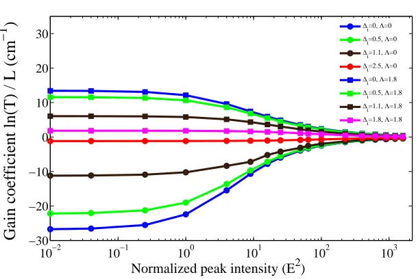
Fig. 1 displays the gain, respectively absorption, coefficient obtained from Eq. (34) in dependence of the input intensity for different detunings. For all curves, it starts at the small-signal value and then drops to the vacuum value of zero due to the generation of carriers and the resulting bleaching. Obviously, the small-signal ab-sorption/gain is highest at∆i=0 and decreases for increasing modulus of detuning

according to Eq. (27). The intensity where saturation becomes apparent seems to increase with increasing modulus of detuning.

Since the ratio ofΓ/γp=4 refers to a Voigt-profile situation where neither

ho-mogeneous nor inhoho-mogeneous broadening are clearly dominating, we fit the de-pendence of the gain coefficient on intensity with different models that describe saturable absorption in the case of two-level systems with inhomogeneous,

α=α0/ q

(1+E2_/E2

s), (36)

and homogeneous,

α=α0/(1+E2/Es2), (37)

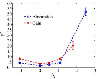
broadening [53]. The latter proves to fit best the simulation. We show in Fig. 2, the modulus squared of the saturation field strength vs∆ias extrapolated from the

above formula. The saturation intensity is minimal at∆i=0 and is slightly different,

about a factor of two, for the gain (E2_{=3.6) and the absorption case (E}2_=1.8).

It strongly increases in both cases for increasing modulus of the detuning, whereas it should be constant in the strongly inhomogeneous limit [53]. As indicated above, a ratio ofΓ/γpcorresponds neither to strongly inhomogeneous broadening nor to

10−2 10−1 100 101 102 103 −30

−20 −10 0 10 20 30

Normalized peak intensity (E2)

Gain coefficient ln(T) / L (cm

−1

)

∆i=0.5, Λ=0

∆i=1.1, Λ=0

∆_i=2.5, Λ=0

∆i=0, Λ=1.8

∆i=0.5, Λ=1.8

∆_i=1.1, Λ=1.8

∆_i=1.8, Λ=1.8

Fig. 1 (Color online) Modal gain coefficient as a function of the normalized intensity in the center of the Gaussian input beam for different values of the detuning in the absorption (circles) and gain regimes (squares). [Adapted from [25]]

and lead to a stronger homogeneous broadening at room temperature than at lower temperatures [54]. Nevertheless, at least in quantum dash samples there is evidence for a strong coherent hole (the equivalent to the so-called Lamb-dip in Doppler-broadened atomic ensembles) at room temperature [55] indicating at least partial in-homogeneous broadening. This coherent hole is observed in other simulations also. Hence it seems to make sense that the saturation behavior shares features known from homogeneous and inhomogeneously broadened systems.

For an experimental situation withwx=15µm andwy=0.5µm,E2=1

corre-sponds to a power of 7.1 mW. Hence the minimum value of the saturation power is 13 mW in the absorption case and 26 mW in the gain case. If instead ofγ=0.15 (or 78 ps lifetime), the purely radiative lifetime is considered, the corresponding values are about a factor of 10 lower and easily accessible experimentally.

As indicated, the simulations presented neglect pump depletion within the medium. We have preliminary results using a split-step beam propagation method [56]. The term ‘split-step’ implies that the simultaneous action of diffraction and nonlinear refraction (determined by χ) in Eq. (32) is replaced by a step-wise scheme of al-ternating diffraction and refraction steps. This works by splitting the medium inm

layers with a thicknessδz=LA/m. The diffraction part is solved in Fourier

(trans-verse wave number) space, the refraction is solved in real space via Eq. (33). In each layer the carrier equations need to be solved providing a significant computational load. We find that for our case,m=16 provides enough resolution (forLA=1 mm)

−1 0 1 2 3 0

5 10 15 20 25 30 35 40 45 50 55 60

∆

i

E

2

Absorption Gain

Fig. 2 (Color online) Modulus squared of saturation field strength (proportional to saturation in-tensity) obtained from a fit of the curves in Fig. 1 to Eq. (36) as a function of detuning. Squares represent the gain case (red online), circles the absorptive case (blue online). The lines are only a guide for the eye. [Adapted from [25]]

the saturation intensity for the absorption increase by a factor of about 1.6 and the saturation intensity for the gain decreases by a factor of about 0.7 (for∆i=0). As

a result, the gain saturates now slightly easier than the absorption. This is easily un-derstandable because the pump depletion due to absorption will hinder saturation in the subsequent layers. On the other hand, the amplification due to gain will help to saturate the gain in the subsequent layers. Similar considerations will be important in Sec. 3 to interpret multi-pass effects.

2.2.3 Results: Self-lensing

One effective method to assess the strength of a χ3- or saturable refractive index

nonlinearity is to look for self-lensing, e.g. in a so-called z-scan geometry [57]. Since the input beam is spatially varying, also the refractive index is. Around the beam center, the variation is necessarily parabolic. According to [58] the radius of curvature acquired by a wave propagating a distanceLain a medium is given by

1

R(r)= 1

r

∂

∂rn(r)La. (38)

From that we can identify an effective focal power:

1

f(x) =−

1

x

∂

∂xn(x)La (39)

=−∆n0La µ

1

x

∂

∂xReχI(x) ¶

If the refractive index distribution would be a pure parabola, the focal power would be constant over the whole beam, thus implying an aberration-free equiva-lent lens. In reality, this is obviously not the case because the pumping Gaussian has an inflection point. Nevertheless the parabola is often a good approximation in beam center where most of the beam energy is. This was studied in detail in atomic vapors [59] and we will discuss it for the QD below. In any case, the curvature will give a quantitative indicator for the strength of beam shaping even if the lens is not perfect. The focusing can be experimentally detected by a change of the beam width in far field [60] or at some distance after the medium [59] (similar as in z-scan tech-niques [57]). In this first treatment, we will confine to a thin lens to demonstrate the principles. For a quantitative description of a real experiment it might be necessary to include absorption and nonlinear beam reshaping during propagation.

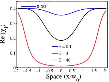
Fig. 3 shows the spatial profile of the real part of the susceptibility imposed by the Gaussian pumping profile for low, intermediate and high peak intensity. For low intensity it follows roughly the Gaussian intensity distribution of the input beam (‘Kerr-limit’) whereas at high intensities there is a broad plateau in beam center because the beam has sufficient intensity to saturate the sample even in the beam wings. At beam center, the variation is parabolic leading to lensing. Fig. 4 shows

−2 −1.5 −1 −0.5 0 0.5 1 1.5 2 0

0.1 0.2 0.3 0.4

Space (x/w

0

)

Re (

χ

)

E = 0.1

E = 3

E = 40 X 10

Fig. 3 (Color online) Spatial profile of the real part of the susceptibility for, from top to bottom line, low (blue line, amplitude enhanced by a factor of 10), intermediate (black line) and high excitation (red line).Λ=0,∆i=1.1. The total excursion is∆n=1.6×10−4_{. [From [25]]}

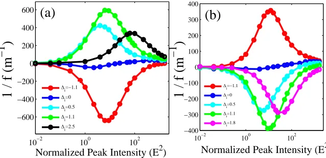
how the lens power change as function of input intensity for different detunings in the absorption case (a) as well as in the gain case (b). Apart from the∆i≈0-case

(discussed separately below), the focal power increases from zero with increasing intensity, reaches a peak at an intermediate intensity and decreases again if the inten-sity is increased further. The sign of the lensing depends on the sign of detuning and whether the sample is absorbing or providing gain, as expected. The maximum lens effect occurs at∆i=1.1 andE2=9 (P=64 mW). The focal power is maximum

intensity needed to obtain maximum lens power increases for increasing modulus of detuning. This is probably due to the fact that the saturation intensity increases with detuning and the maximum effect is found for the same saturation condition.

10−2 100 102 −600

−400 −200 0 200 400 600

Normalized Peak Intensity (E2)

1 / f (m

−1

)

1 / f (m

−1

)

10−2 100 102 −400

−300 −200 −100 0 100 200 300 400

Normalized Peak Intensity (E2)

∆_i=−1.1

∆i=0

∆_i=0.5

∆_i=1.1

∆i=2.5

∆_i=−1.1

∆_i=0

∆i=0.5 ∆_i=1.1

∆_i=1.8

(b)

(a)

Fig. 4 (Color online) a) Focal power as function of normalized peak intensity for different detun-ings in the absorption case (a) and the gain case (b). (Λ=1.8 was chosen because it reproduced the experimental finding that maximal gain is about half the absorption coefficient.) [From [25]]

The fact that the maximum focal power is obtained at intermediate input intensity can be explained by looking at Fig. 3. For low intensity the curvature follows the curvature of the input profile (‘Kerr-limit’,∆n(x)∼ |E|2_{(x)), but the total effect is}

low because the excursion from the background refractive index is small (note that the curve is blown up by a factor of 10). For high intensity, the excursion is large (Re(χI)becomes nearly zero) but the total focal power is again low because the

curvature is strongly reduced. This is due to the fact that saturation is effective over a large area at high intensities. The case of intermediate intensity is in between: On the one hand the excursion is of reasonable size, about half the maximal effect, on the other hand the curvature is still quite close to the one of the input beam. Both is characteristic for intensity levels around the saturation intensity, i.e. for the onset of saturation, and hence the total effect is maximal. Similar characteristics were found for atomic vapors [59]. Here, in the homogeneously broadened case, it can be demonstrated analytically that maximum focal power is found at the saturation power [59].

The lensing effect is minimal at∆i=0. Indeed, in a purely two-level system no

effect at all is expected for∆i=0 because the contributions of blue and red detuned

In the peak, the predicted lensing effect is actually quite substantial, |fmin| ≈

1.7 mm, in a sense, because the focal length reaches the length of the medium (as-sumed to beLa=1 mm), i.e. the point where the approximation by a thin lens

be-comes questionable. These values were calculated assuming an input beam radius of

wx=15µm chosen because it would be conveniently to work with experimentally

and being somewhat larger than typical fundamental mode sizes in edge-emitting lasers, i.e. in a range where filamentation phenomena might occur. The size of cav-ity solitons is also in that range (about 10µm [30, 61]).

Nevertheless, it turns out that an experimental confirmation is not straightfor-ward: The modification of the input beam by the lensing of the sample can be de-tected by either measuring the on-axis amplitude (being proportional to the square of the new beam waist of the transmitted beam,w02

x) or the beam width in far field

(∼1/w02_x) [60] or, more sensitively, by measuring the beam size either directly or via the transmission through a pinhole at some suitable chosen distance after the medium as it is done in usual z-scan techniques [57]. Replacing the medium by a thin lens of focal length f, the size of the new beam waistw0

xcan be calculated by

ABCD-matrix theory as

w0_x=wx 1

1+ πw4x λ2_f2

. (41)

For an input beam waist ofwx=15µm and a thin lens with f ≈1.7 mm, the new

beam waist iswx=14.3 µm at a distance of 0.16 mm. This rather small change

in beam is quite difficult to detect. Eq. (41) says that the effect becomes more pro-nounced if the initial beam radius is increased (at constant f), being substantial if the Rayleigh length of the input beamzr=πw2x/λ is of the order of f. In reality,

however, the focal length scales like f ∼w2

x, since, as discussed for Fig. 3, the

cur-vature of the susceptibility profile follows the curcur-vature of the input beam in first approximation for not too strong saturation (see [59] for an analytical treatment). Hence, actually the strength of the detected signal can’t be influenced by choice of the input beam size.

However, due to the approximately quadratic dependence of the new beam waist on ratio ofw2

x/f, the situation rapidly improves with increasing focal power. For

example, a change of size by 20%, which should be experimentally detectable, is reached already for a focal power of about 1000/m, i.e. only about two times the maximum value reported in Fig. 4.

the carrier density needs to be spectrally and spatially resolved in our case. We did some test runs using a lifetime of 0.5 ns which yield an increase of 10% in saturation and negligible effect in lensing. Note that the influence of the lifetime on the scaling of the saturation power can be treated exactly without additional calculations (as discussed above) due the way the equations are scaled.

−10 −5 0 5 10

−0.4 −0.2 0 0.2 0.4 0.6

∆

i

1/2 (

χ I

)

Im(χ) Γ/γ_p=1 Re(χ) Γ/γ

p=1

Im(χ) Γ/γ

p=4

Re(χ) Γ/γ_p=4 Im(χ) Γ/γp=10

Re(χ) Γ/γ

p=10

Fig. 5 (Color online) Real and Imaginary part of the linear susceptibility as function of detuning for different ratios between inhomogeneous and homogeneous broadening. [From [25]]

Finally, Fig. 5 shows how real and imaginary part of the linear susceptibility change as function of detuning for different ratios between homogeneous and inho-mogeneous broadening. Since the linear susceptibility defines the maximum value of the nonlinear index change, this provides a good guidance on the maximum effect to be expected. Choosing a ratio ofΓ/γp=10 instead of 4 decreases the maximum

of the real part of the susceptibility by a factor of 2.1. For a ratio ofΓ/γp=1, it is

a factor of 2 higher. Hence, at constantγp, one can expect to benefit from improved

growth with a reduced inhomogeneous broadening. Note that increasingγpat

con-stantΓ is not beneficial because the increase of the scaled susceptibility is sublinear (cf. Fig. 5) and is overcompensated by the dependence of the proportionality factor between scaled and unscaled susceptibility onγp, see Eq. (24). We conclude that

though uncertainties in the relaxation constants will influence the measurements quantitatively, our overall conclusion that the lensing is at the edge of being de-tectable is not changed. One reason for the somewhat low nonlinear phase shift is the inhomogeneous broadening. The peak phase shift from Fig. 5 forΓ/γpis only

40% of what a homogenously broadened transition with the same total QD density would give.

contribution of an ES 100-120 nm away from the GS (roughly the situation in InAs QD) will partially overlap and counteract the effect of the GS transition: With an inhomogenous broadening ofΓ ≈40 m the distance between the ES and the GS on the∆I-axis in Fig. 5 is 3. (The contribution is smaller for the imaginary part of the

susceptibility (our main focus in the experiment later) because that tails off fast than the real part with detuning.) In particular that implies that there might be a nonzero α-factor around the gain peak of the GS due to the off-resonant contributions from WL and ES. Though there are reports of fairly lowα-factors [35, 36, 37] on the one hand, there is also significant evidence of contributions from the other states, discrete or continuous (WL or barrier based), whose contribution to the refractive index in particular could be significant for high injection values (and thus large carrier densities in the ES or WL) [38, 39, 40]. Modeling more complex contribu-tions has been dealt with by means of properly balanced rate–equacontribu-tions models for the carriers and/or by inclusion of a contribution from the continuum and discrete states in WL and QD either in a semi-phenomenological or more first-principle way [39, 62, 63, 64, 65].

2.3 Numerical results: Cavity dynamics

2.3.1 Nonlinear refractive index andα-factor

As just discussed, theα-factor is an important, but still controversial factor in QD-based photonic devices. It depends very much on operating conditions and also on measurement method (see, e.g., the discussion in [39]). Commonly used techniques to measure theα-factor (e.g. [39]) are based on the FM/AM response of the laser output or the amplified spontaneous emission spectrum to a small modulation or variation of the injection current using the relation

αH= dReχ

dN dImχ

dN

, (42)

where the change in carrier density (being it in the QD or the WL) is introduced via the variation of current around some working point. In another method one analyzes the output of a laser with injection [66]. Since this latter method can be easily de-scribed by our formulation, Eq. (30), we use it here to point out one aspect of the carrier dynamics leading to an asymmetric gain spectrum and hence a nonzeroαH

at gain peak in addition to the off-resonant effects of the WL and ES states. This is the different thermal occupation of the size dispersed QD GS states described by the factorβintroduced in Eq. (18).

broadening does not influence the symmetry but decreases only the peak effect (as discussed above).

Fig. 6 Plot of the real and imaginary parts of the susceptibility spectrum versus the detuning from the QD population line center forβ=0 and for five values of the pumpΛ from absorption to gain. Other parameters for these simulations areσcape,h=500,γesch =100,γesce =0.01,Bhe,eh=500, γp=15,Γ=60,Γsp=2.5,γnr=γnrW L=0.15,C=25,Θ=−2,|E|=20. [From [24]]

Fig. 7 shows the situation forβ =0.02. Whenβ >0, the gain spectrum shows an asymmetry steadily growing withβ and with carrier injectionΛ (Fig. 7b) thus implying a nonvanishingα-factor. The real part of the susceptibility (Fig. 7a) is less affected, the point where all dispersion curves approximately intersect and hence whereαH≈0 moves to slightly positive detuning (here∆i≈0.015).

Fig. 7 Plot of the real and imaginary parts of the susceptibility spectrum versus the detuning from the QD population line center forβ=0.02 and five values of the pumpΛfrom absorption to gain. Other parameters as in Fig. 6. The inset is a blow-up of the curve forΛ=2.4. [From [24]]

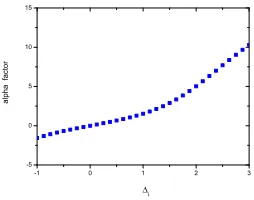
the resulting differentials numerically. For a bias ofΛ=2.36 (pump slightly below transparency) andβ =0.01, we plot its value in Fig. 8.

-1 0 1 2 3 -5

0 5 10 15

a

l

p

h

a

fa

ct

o

r

i

Fig. 8 α-factor versus the detuning from the QD population line center forβ=0.01 andΛ=2.36. Other parameters as in Fig. 6 exceptC=20,Θ=−3,|E|=30.

By inspecting it, we see that for fixed current pump (below threshold) and in-put field values, the system exhibits a negativeα-factor for higher energy (smaller wavelength) spectral values, consistently e.g. with [62], which increases to positive values, again, with a behavior qualitatively not dissimilar from the ones reported e.g. in Fig. 6 of [67], and experimentally in [66]. The dispersion curve is strongly asymmetric, though the zero point is actually not much shifted for this relatively low values ofβ.

2.3.2 Nonlinear phase shift and Fabry-Perot fringes

We discussed in Sec. 2.2.3 self-lensing as a possible method to assess the nonlin-ear, intensity-dependent, phase shift and found that it is close to the detection limit. Interferometric methods are an attractive alternative in which a probing beam after having passed the QD sample might be interfered with a reference beam. Alterna-tively, one might measure the shift of cavity resonances with intensity. Note that contrary to the way theα-factor is normally measured, i.e. by changing the carrier density via changing the injection current (see previous section), we are interested here in the index shift generated by a coherent light beam via the carriers it generates (or takes out via stimulated emission).

In a Fabry-Perot cavity a refractive index change of δn causes a shift of the wavelength resonance by

δ λ=λ0δn

nb, (43)

whereλ0 is the resonance wavelength belonging to the background index nb. In

order that a shift is detectable, it should be about half of a free spectral range (FSR) of the cavity given by∆ λFSR=λ02/(2nbL). From this the detectable refractive index

δn=λ0

4L. (44)

For the simulation parameters used in Sec. 2.2.1, the maximum index shift is 1.6× 10−4 at 1280 nm. Hence, the nonlinear shift should be detectable in cavities of length of 2-4 mm. Note that this is only a rough estimation. On the one hand a shift of the fringes of less than half a FSR is detectable, on the other hand, the numbers given assume optimal tuning for the maximal index effect (Fig. 5) and complete saturation.

2.3.3 Optical Bistability

The set of equations proposed in Sec. 2.1 can be directly exploited to investigate the stationary emission states of a microresonator with coherent injection. In particular, an interest resides in the regimes where the stationary curve has a bistable character. This issue is interesting ‘per se’ for all-optical processing applications, but also because bistability is the fingerprint of highly nonlinear regimes and has also been investigated in relation to the search for modulational instabilities leading to pattern formation and cavity solitons (see, e.g., [27, 28, 29] for reviews).

0 10 20 30 0 10 20 30 |E | ( A r b . U n its) |E i | (Arb. Units) C=12

C= 8 C= 9

a)

0 10 20 30 40 50 0 10 20 30 |E | ( A r b . U n its) |E i | (Arb. Units) C=15

C= 11 C=10

b)

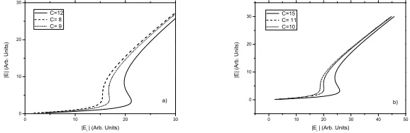
Fig. 9 Bistable and monostable steady state curves for the intracavity vs injected field amplitudes: a) resonant caseθ=∆i=0 withC=12,9,8 (respectively, full, dotted and dashed lines) repre-sentatives of bistable, threshold and monostable regimes; b) dispersive caseθ=−1,∆=0 with

C=15,11,10 (respectively, full, dashed and dotted lines); representatives of bistable, threshold and monostable regimes. Other parameters as specified in the text.

In this research, the mainstream of the experimental investigations has been per-formed in absence of carrier pumping and with an injection resonant with the QD centerline and the cavity reference frequency (purely absorptive regime); in Fig. 9a we show the steady state field curves for the caseθ =0,∆i=0 and we evidence

the existence of a threshold in theCparameter, approximatively equal to 9, below which the curve is monostable. Other parameters in the simulations are the same as in Subsec. 2.3.1.

dimin-ished fraction of the spectral population distribution resonant with the external drive, as reported in Fig. 9b. The threshold for C is close to 11 for this case. Note that, there being no analytical expression for the steady states of the population variables, the threshold must be calculated by integrating the dynamical model to a stationary regime and identifying the curve where extrema disappear.

Globally, our model predicted bistability forCvalues of about 10-20 [23], within experimental reach, in principle. The cooperativity parameter of the edge-emitting InAs-based structure investigated in Sec. 3 is estimated to be about 5 (with back-ground waveguide losses of 1.5/cm determined for devices of this kind), i.e. roughly half the requirement for bistability. The analysis of Fig. 11 suggest an optical den-sity of onlyα0≈14.5/cm givingC≈3. The InAlAs-based structure investigated in

Sec. 4 is estimated to be about 7 (assuming the same background losses) or about 3, assuming losses of 10/cm suggested by the analysis in Sec. 4.2.2. This means all present samples fall short of the requirement for bistability, but an optimization in terms of length and/or an improvement in growth density, number of layers or a re-duction in inhomogeneous broadening should open suitable parameter regimes (see also the discussion in Sec. 5).

The determination of the C parameter required for pattern formation has been dis-cussed in [24] and suggested that QD densities needed (via Eq. 31) for such scopes are not outside reach. More precisely, pattern formation is predicted in the order of NQD≈1012cm−2(longitudinally integrated density for vertical-cavity devices)

[22].

3 Experiments on InAs/GaAs quantum dots around 1250 nm

3.1 Devices and experimental setup

The investigated sample is a quantum dot diode (QDD) from Innolume GmbH with a cavity length ofL=1.5 mm. It contains ten layers of InAs QD in a GaAs matrix. The epitaxial structure is similar to the one described in [9]. A single-mode ridge-waveguide ensures spatial fundamental mode operation. The device is designed as a laser with a front reflectivity ofR1=0.18 and a back reflectivity ofR2=0.99. The

light-current (LI) characteristic is shown in Fig. 10, from which a threshold current ofI=26.6 mA atT =15◦_{C is inferred. However, in our investigations, it is used} only in absorptive mode (i.e. without current injection) or as an amplifier below threshold.

0 50 100 150 200 250 300 0 50 100 150 o u t p u t p o w e r ( m W ) current (mA) a)

1230 1240 1250 1260 1270 1280 0 0.2 0.4 0.6 0.8 1

x 10−10

Wavelength (nm)

Intensity (Arb. Units)

5 mA 10 mA 24 mA

(b)

Fig. 10 (Color Online) a) LI-curve (squares) of device with linear fit (straight line),T =15◦_C.

b) Spontaneous emission spectra from the QDD for different injection currents below threshold. [Adapted from [41]]

improves. We choose a current of 24 mA for the detailed investigations under gain conditions.

1260.41260.51260.61260.71260.81260.91261.0 0.0 0.1 0.2 0.3 0.4 0.5 0.6 0.7 r e f l e c t e d s i g n a l ( a r b . u n i t s ) wavelength (nm) a)

-10 -5 0 5 10

phase 0.00 0.05 0.10 0.15 0.20 0.25 reflectivity b)

Fig. 11 (Color Online) a) Linear reflection spectrum of QDD (squares) displaying Fabry-Perot fringes and fit to a sine-wave (T=15◦_{C,I=0 mA). b) Calculated Airy-function in reflection for}

a Fabry-Perot interferometer forR1=0.18,R=0.99 and internal (intensity) losses of 16/cm.

Fig. 11a shows a linear reflection spectrum of the QDD obtained from a tun-able laser (Santec TSL-210V). The free spectral range is fitted to be 0.15 nm in agreement with the length specification of the QDD by the manufacturer. The ap-parent Finesse is about 1. Finesse and modulation depth can be approximately fitted by a modal loss of 16/cm (see Fig. 10b), somewhat less than the 28.2/cm (1.5/cm waveguide loss and 26.7/cm absorption) expected from structures of this kind from Sect. 2.2.1, but indicating still a very reasonable interaction strength.

longitudi-Spectrometer

_BS

OI PD1

PD2 L2

L1 BS1

OSA PC

10/90

MO C1

C2

M M

Temp. Contr.

QDD

APP

M

(a)

cs

xx

Cr

4+

:Fr

1273.8 1274.1 1274.4 1274.7 0

0.5 1 1.5 2

x 10−5

Wavelength (nm)

Intensity (Arb. Units)

(b)

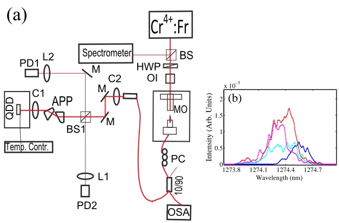
Fig. 12 a) Experimental setup: Chromium forsterite laser (Cr4+_{:Fr), beam splitter (BS, BS1),}

half-wave plate (HWP), optical isolator (OI), microscope objective (MO, 40×), optical spectrum ana-lyzer (OSA), mirror (M), anamorphic prism pair (APP), aspherical collimator (C1,f=3 mm; C2,

f=13.9 mm), lenses (L1, f=50 mm; L2, f=35 mm), amplified photodiode (PD1, PD2). b) Examples for variation of spectra of Cr:Fr laser over time. [Adapted from [41]]

nal modes of the QDD. Hence, the coherence length of the Cr:Fr laser is less than the QDD cavity length and cavity resonance effects are expected to be weak. Since the laser is not optimized for cw operation, its modal envelope fluctuates slightly over time (some typical examples are shown in Fig. 12b). However, the fluctuations are small against the spectral broadening of the QD, which is on the several nm to tens of nm level.

Then the beam is coupled into the QDD with an aspherical lens (C1). The proce-dure for the coupling is actually the opposite: The light coming out from the QDD diode is fiber coupled first, with an efficiency of 37%. Then we can conclude that the effective coupling efficiency of the Cr:Fr beam coupled out of the fiber to the QDD waveguide isce f f =0.37. The data given below uses the raw data, i.e. the

power incident on the device.

The light reflected by the sample and the light coming out of it is collected via a beam splitter (BS1, Fresnel reflection of 1% from front surface, back surface AR-coated) and focused onto the output photodiode (PD1). A similar photodiode mon-itors the input beam as well (PD2). In the experiment, the incident power is varied by turning the half-wave plate and PD1 and PD2 are simultaneously monitored with a digitizer with 16 bit resolution. The reflection coefficient is derived from the ra-tio of the signal of the two detectors taking the known offsets and sensitivities into account. We plot in the followingR(in logarithmic scale) and lnR(in linear scale) because lnRshould relate to the absorption (gain) coefficient as displayed in Fig. 1 without multi-pass effects, i.e. for a device with perfect anti-reflection coated in-put facet. Note that in [41] the data were presented as gain (absorption) coefficient per unit length withL=1.5 mm in order to facilitate comparison with usual gain coefficients, but we prefer not to do the conversion here due to its strong limitations.

3.2 Experimental results on saturation of gain and absorption

Fig. 13(a) shows how the gain coefficient changes as function of input power for λ =1245 nm under gain,I=24 mA, and absorptive conditions,I=0 mA. The reflection coefficient from the QDD shows a pronounced power dependence starting at power levels slightly less than 10 mW for the absorptive case indicating bleaching of absorption. The reduction of reflectivity due to gain depletion sets in somewhat earlier. Fig. 13(b) shows the corresponding curves forλ=1255 nm showing similar trends.

The same holds for Fig. 14a displaying the situation forλ = 1265 nm though the small-signal intercepts seem to be slightly reduced. This effect is much stronger in Fig. 14b displaying the data for λ = 1280 nm. This is due to the increased detuning to line center. Under gain conditions, there is still a saturation effect, but the absorption is essentially constant (the small decrease at high power is probably an experimental artefact).

0.1 1 10 100 −3

−2.25 −1.5 −0.75 0 0.75 1.5

Power (mW)

Ln (R)

0.1 1 10 100

−3 −2.25 −1.5 −0.75 0 0.75 1.5

Power (mW)

Ln (R)

0.05 0.11 0.22 0.47

1 2.12 4.48

0.05 0.11 0.22

0.47 1 2.12 4.48

(a)

_(b)

R R

Fig. 13 (Color Online) Reflection coefficient as function of input power [dark gray (blue) data points forI=24 mA, light gray (red) data points forI=0 mA] and fit to an inhomogeneous broadening model [dark gray (red) line forI=24 mA, light gray (blue) line forI=0 mA). (a)

λ = 1245 nm, (b)λ = 1255 nm. [Adapted from [41]]

and homogeneous, Eq. (37), broadening. The results shows that both models fit the data atλ = 1255 nm andλ = 1265 nm quite well but the inhomogeneous model proves to fit better and is the only model that fits the data well atλ = 1245 nm and λ =1280 nm, Fig. 13(a), Fig. 14(b).

Fig. 15 shows the saturation power under absorptive and gain conditions as func-tion of wavelength as obtained from the fits displayed in Figs. 13, 14. The minimum saturation power is reached atλ = 1255 nm, i.e. line center, as expected, and is

Psat = 9 mW in the absorptive case andPsat = 1.4 mW in the gain case. The

sat-uration power increases for increasing detuning. These tendencies are in qualitative agreement with the simulations presented in Sect. 2.3.

3.3 Analysis and discussion

Via Isat =2Psatce f f/(πwxwy), where Psat are the saturation powers reported in

Fig. 15 andwx =3×10−6m andwy =0.5×10−6m are the beam radii in the slow,

0.1 1

10

100

−2.25

−1.5

−0.75

0

0.75

Power (mW)

Ln (R)

0.1 1 10 100

−2.25

−1.5

−0.75

0

0.75

Power (mW)

Ln (R)

2.12

1

0.22

0.11 0.47

0.22

0.11 2.12

1

0.47

R

R

(b)

(a)

Fig. 14 (Color Online) Gain coefficient as function of input power at (a)λ = 1265 nm, (b)

λ = 1280 nm. Legend as in Fig. 13. [Adapted from [41]]

12400 1250 1260 1270 1280 1290 10

20 30 40

Wavelength (nm)

Saturation Power (mW)

Absorption Gain

Fig. 15 (Color Online) Saturation power as function of wavelength in absorption and gain cases. [Adapted from [41]]

is obtained for the absorptive case. This value agrees with numerical predictions using the parameters from Sect. 2.3 and Eq. 22 for a carrier lifetime in the ground state of 60 ps, i.e. a rather small value.

A qualitative difference between the experimental results and the simulations is that in the simulations the absorption saturates earlier than the gain, i.e. the theo-retical expectation for the gain case based on Sect. 2.3 isIsat = 2.8×109W/m2,

This feature, as well as the absolute scaling of the reflection coefficients, is strongly influenced by the fact that the sample does not have AR-coatings on both ends but the coatings are designed for laser operation. As indicated, we don’t expect strong cavity resonance effects because of the low coherence length of the input laser, but nevertheless the device will behave as a two-pass amplifier due to the high reflectivity of the back mirror. Some portion of the light attenuated or amplified after one double pass 2Lwill be in turn retro-reflected into the sample due to the finite reflectivity of the front facet. The expected total reflectivity can be estimated from the incoherent sum of intensities of the multi-pass configuration,

R=R1+ceff(1−R1)2 R2e

(−αg+g)2L

1−R1R2e(−αg+g)2L

, (45)

whereαg≈1.5/cm represents the waveguide loss andg=−α is the modal gain

coefficient. (Qualitatively similar results are obtained if one averages the coherent Airy function over the resonator phase.) The corresponding function is displayed in Fig. 16 as the curved solid curve.

-30 -25 -20 -15 -10 -5 0 5 0.1

1 10

R

g / cm

Fig. 16 (Color Online) Reflection coefficient calculated from Eq. (45) versus modal gain coeffi-cient [Light gray (red) solid line]. Dashed lines: Value for high power asymptote (g=0). Solid black line: Estimated maximal linear gain. Dotted lines: Reduction of linear absorption and gain by factor of√2.

Obviously, the small-signal coefficient in the absorptive case (g≈ −27/cm) is totally determined by the reflectivityR1≈0.18 of the front facet. This is in rough

effects explain also the difference in saturation power between gain and absorp-tion: A change of modal gain from 6.5/cm to only 5.7/cm is required to change the externally observed reflection coefficient by a factor of√2, whereas the modal absorption needs to change from−27/cm to−4.6/cm to achieve the same effect. This is easy to understand hence absorption will reduce the intensity propagation further down into the structure and thus hinder saturation. In contrast, with gain the intensity increases with propagation in the structure and hence saturation becomes easier. Hence, the multi-pass effects delay saturation in absorption and favor it in gain explaining the observed asymmetry.

10 -4 10 -3 10 -2 10 -1 10 0 10 1 10 2 10 3 10 4 10 5 -2.0 -1.5 -1.0 -0.5 0.0 0.5 1.0 1.5 2.0 g a i n ( 1 / c m )

normalized peak intensity E

2

Fig. 17 (Color Online) Reflection coefficient calculated from Eqs. (45), (36) versus normalized intensity. Black line:g(0) =−27/cm, red (light gray) line:g(0) =−14.5/cm, blue (dark grey) line:g(0) = +6.5/cm. Dashed lines denote fits of these plots to the saturation law (36) and are essentially not distinguishable from the data.

One can now use the saturation law (36) to supply the intensity dependence ofg

in (45). The resulting reflection coefficient is displayed in Fig. 17 for different small signal absorption and gain values. It is apparent that the curves have a qualitative similarity to the experimental curves in Fig. 13. Furthermore, they can be essentially perfectly fitted by the saturation law (36). From the fit one obtainsE2

s =0.29 for the

gain case,g(0) = +6.5/cm, andE2

s =33.3 for the absorptive case,g(0) =−27/cm.

This confirms the asymmetry between saturation of absorption and gain discussed above, but the ratio between these values is very high, about 110, whereas the ex-perimentally observed ratio is significantly smaller, around 7. It turns out that these values are very sensitive to the total absorption, e.g. forg(0) =−14.5/cm (inferred earlier from Fig. 11)E2

s =9.6. This is reasonable since the depletion of the pump –

and hence the delay of saturation – will be stronger, if the linear absorption coeffi-cient is stronger. For this value ofg(0)the ratio between the saturation intensity of gain and absorption is about 30, still larger than in the experiment. In view of the un-certainties, one cannot make strong statements but it appears that the ‘material’ (i.e. not influenced by multiple-pass effects) saturation intensity is about 5×108_W/m2_,

correspond to a lifetime of the GS of 170 ps, which is a low though still reasonable value.

For SESAM applications, saturation fluences for 1280-1340 nm QD under short-pulse excitation are reported to be 0.02-0.25 J/m2_{[8, 7, 18]. If the carrier decay}

within the width of the probing pulse can be neglected, the saturation fluence can be converted to an equivalent cw saturation intensity by multiplying it with the carrier decay rate. Hence for a lifetime of 100 ps one concludes on saturation intensities of (0.2−2.5)×109_W/m2_{in line with our observation.}

3.4 Experiments addressing nonlinear index shifts

As indicated from the discussion above, the data for the saturation of the imaginary part of the refractive index (i.e. gain or absorption) would be much cleaner and more straightforward to analyze if the sample would have been AR-coated at both input facets (or the waveguide would have been tilted with respect to the facets). The choice for a laser samples instead of an AR-coated amplifier stemmed from the desire to probe nonlinear index shifts via the shift of Fabry-Perot fringes as explained in Sect. 2.3.1.

We briefly describe the experiment. A low-amplitude beam of a tunable laser was injected into the other input of the 90:10 fiber splitter. It is scanned over 0.5 nm, i.e. several FSR of the QDD, and its reflection is measured in presence of the strong pump laser. The tunable probe beam is chopped at a frequency of 800 Hz and its weak signal is filtered out of the total reflection signal with the help of a lock-in amplifier. We observe a change in shape and Finesse of the Airy function, i.e. a non-linear version of Fig. 11a, dependent on the pump power, which is qualitatively as expected. This indicates that the idea of the measurement works in principle. How-ever, the shift is about 0.001 nm/mW (external power) independent of wavelength and current. As one expect a different sign of the shift under absorptive and gain conditions, we conclude that we don’t probe a carrier effect but some background absorption. For comparison, the fringe shift with temperature was determined to be 0.1 nm/K, i.e. the effect can be caused by very small temperature variations. The origin of this shift is unclear at the moment.

4 Experiments on InAlAs/GaAlAs quantum dots at 780 nm

height may be obtained by evenly incorporating aluminium in both the barrier and the dot materials leading to a higher confinement of quantum states and to the for-saken spectral overlap with the GaAlAs system. In this framework, InAlAs/GaAlAs QD [70, 71] open very promising perspectives both for cw and pulsed nonlinear or even self-organizing optical systems. In this section, structural and optical proper-ties of MBE-grown InAlAs/GaAlAs quantum dots are investigated as a function of the growth kinetic and thermodynamical conditions. Appropriate choice of growth conditions allows to control the density as well as the average size of QD. This es-tablishes also an excellent approach for controlling the carrier lifetimes during the growth stage, and introduces means of realizing either a slow focusing Kerr effect (FKE) material (ns-scale) or a fast (ps-scale) saturable absorber, as started in [12].

In this section, we report on linear and nonlinear measurements of the suscepti-bility of InAlAs/GaAlAs QD, after describing their growth conditions, which cor-relate to their structural properties in terms of dot and dislocation densities. Optical quality is established through spectral and temporal photoluminescence (PL) mea-surements. The core of the section is dedicated to the measurement of group index and nonlinear absorption using a long (high-order) Fabry-Perot cavity embedding InAlAs/GaAlAs QD. This approach leads to unprecedented measurements for this material and establishes, though not yet fully exploited, quite an efficient saturation behavior.

4.1 Description of the experiments

4.1.1 Material properties and device structure

The sample was MBE-grown on a GaAs substrate, using the Stransky-Krastanov growth regime. According to the criteria developed in the model, Sec. 2.1, there is a necessity to obtain a large volume of interaction between QDs and light by increas-ing the overall density of dots, and thereby the sensitivity of our experimental setup to the QD contribution to the susceptibility. This was found in growing five super-imposed planes of In0.67Al0.33As QDs with Ga0.67Al0.33As barriers as the nonlinear

material (Fig. 18a). The symmetric step-graded barrier and cladding layers with cor-responding material concentration follow and a GaAs cap terminates the structure. A cross-sectional visualization of QD was performed that gave information on the relaxation degree of the QDs which revealed appropriate for optical experiments. Due to the depth at which QD layers are located with respect to the surface, the den-sity of dotsρDcould only be inferred from a cross-sectional TEM image and lead to

an integrated density for the 5 layers such as 2×1011_<ρ

D<5×1011cm−2.

One-layer samples grown under nominally the same growth conditions had a density of about 2×1011cm−2.