White Rose Research Online URL for this paper: http://eprints.whiterose.ac.uk/82789/
Version: Accepted Version Article:
Gao, J, Holden, J and Kirkby, M (2015) A distributed TOPMODEL for modelling impacts of land-cover change on river flow in upland peatland catchments. Hydrological Processes, 29 (13). pp. 2867-2879. ISSN 0885-6087
https://doi.org/10.1002/hyp.10408
[email protected] https://eprints.whiterose.ac.uk/ Reuse
Unless indicated otherwise, fulltext items are protected by copyright with all rights reserved. The copyright exception in section 29 of the Copyright, Designs and Patents Act 1988 allows the making of a single copy solely for the purpose of non-commercial research or private study within the limits of fair dealing. The publisher or other rights-holder may allow further reproduction and re-use of this version - refer to the White Rose Research Online record for this item. Where records identify the publisher as the copyright holder, users can verify any specific terms of use on the publisher’s website.
Takedown
If you consider content in White Rose Research Online to be in breach of UK law, please notify us by
A distributed TOPMODEL for modelling impacts of
1
land-cover change on river flow in upland peatland
2
catchments
3
Jihui Gao, Joseph Holden, Mike Kirkby 4
water@leeds, School of Geography, University of Leeds, Leeds, LS2 9JT, 5
UK 6
7
Abstract
8
There is global concern about headwater management and associated 9
impacts on river flow. In many wet temperate zones peatlands can be found 10
covering headwater catchments. In the UK there is major concern about how 11
environmental change, driven by human interventions, has altered the 12
surface cover of headwater blanket peatlands. However, the impact of such 13
land-cover changes on river flow is poorly understood. In particular, there is 14
poor understanding of the impacts of different spatial configurations of bare 15
peat or well-vegetated, restored peat on river flow peaks in upland 16
catchments. In this paper, a physically-based, distributed and continuous 17
catchment hydrological model was developed to explore such impacts. The 18
original TOPMODEL, with its process representation being suitable for 19
blanket peat catchments, was utilized as a prototype acting as the basis for 20
the new model. The equations were downscaled from the catchment level to 21
the cell level. The runoff produced by each cell is divided into subsurface 22
flow and saturation-excess overland flow before an overland flow calculation 23
takes place. A new overland flow module with a set of detailed stochastic 24
algorithms representing overland flow routing and re-infiltration mechanisms 25
was created to simulate saturation-excess overland flow movement. The 26
new model was tested in the Trout Beck catchment of the North Pennines of 27
England and found to work well in this catchment. The influence of land 28
cover on surface roughness could be explicitly represented in the model and 29
the model was found to be sensitive to land cover. 30
31
Keywords: blanket peat, flooding, peak flow, overland flow, vegetation cover 32
1 Introduction
34
Altering vegetation cover may affect river regimes due to changes in the 35
overall water balance (inputs versus outputs) and also because of changes 36
to flowpaths for water to the river channel. Understanding the impact of 37
vegetation cover and management on the shape of storm hydrographs and 38
the magnitude of flow peaks is vital to support land management decisions 39
(Wheater and Evans, 2009). 40
Peatland landscapes are particularly sensitive to slight shifts in local 41
hydrology or chemistry in which can alter species composition and hence 42
surface cover (Bragg and Tallis, 2001). Peatlands cover around 3% of the 43
Earth’s land surface (Immirzi et al., 1992) and as peatlands are more likely 44
to form in regions with high precipitation excess, they often form in upland 45
areas of the temperate and boreal zones (Gallego-Sala and Prentice, 2013). 46
Large areas of the UK uplands are covered by blanket peat. Blanket 47
peatlands typically have shallow water tables (Price, 1992; Evans et al., 48
1999), and hence the potential for peat to store additional fresh water and 49
act as a buffer to flooding may be very limited (Holden and Burt, 2003; 50
Holden, 2005). Thus a little rainfall can cause rapid saturation of the peat 51
and lead to the generation of saturation-excess overland flow or rapidly-52
flowing near-surface throughflow and these flows may dominate the river 53
hydrograph during storm events (Holden and Burt, 2002). The river regime 54
of blanket peatlands tends to be very flashy with rapidly rising hydrographs, 55
high flow peaks and very little baseflow (Price, 1992; Evans et al., 1999). 56
There are concerns that land management interventions in upland peatlands 57
in the UK may increase flood peaks (e.g. Parrott et al., 2009; Wheater and 58
Evans, 2009; Hess et al., 2010). However, given that these systems are 59
already very flashy in nature it is not clear what impacts such interventions 60
might have. There is also the related problem of the spatial distribution of 61
management interventions. As noted by Holden (2005), the same 62
intervention may both theoretically increase and decrease the flood peak in 63
the main river channel depending on how the intervention affects the timing 64
of water delivery and its synchronicity from different parts of the catchment. 65
There is therefore a need to understand such issues and assess them to 66
support environmental decision making. 67
In many areas of the UK uplands there has been a history, over at least the 68
last 60 years, of vegetation loss attributed to vegetation burning, 69
overgrazing, atmospheric pollution and other interventions (Bower, 1962; 70
Sphagnum or the complete loss of surface vegetation altogether may lead to
72
changes in water movement over peatland surfaces. It is thought that 73
downstream discharge from peatlands might be sensitive to surface 74
vegetation cover change (Holden et al., 2008; Grayson et al., 2010; Ballard 75
et al., 2011; Lane and Milledge, 2013). Vegetation cover and associated
76
surface roughness could be more important to flow peaks in many 77
headwater peatlands than change brought about by other management 78
interventions such as drainage for which studies have often resulted in 79
equivocal conclusions (Holden et al., 2004). Sphagnum is associated with a 80
much greater surface roughness than bare peat and it therefore has an 81
ability to significantly slow down the velocity of water movement (Holden et 82
al., 2008). Peatland restoration efforts are underway across many degraded
83
upland landscapes and these often seek to revegetate bare peat (Parry et 84
al., 2014). Practitioners are very keen to understand whether such
85
revegetation has an impact on river flows (e.g. IUCN, 2011). Thus, we need 86
a tool to evaluate the impact on river flow peaks of changes to, and the 87
spatial distribution of, land cover types in headwater peatlands. 88
TOPMODEL was originally developed by Beven and Kirkby (1979), and 89
initially employed in UK small catchments (Beven et al., 1984). The model is 90
considered as a set of conceptual tools which can be utilised to model the 91
hydrological processes (especially the dynamics of surface and subsurface 92
contributing areas) in a relatively simply way (Beven, 1997). TOPMODEL 93
has been treated as a standard model for hydrological analysis in many 94
parts of the world (e.g. Franks et al., 1998; Lamb et al., 1998; Güntner et al., 95
1999; Peters et al., 2003). 96
The assumptions of TOPMODEL (Beven and Kirkby, 1979) fit the case of 97
blanket peat catchments well, in which river flow is dominated by surface or 98
near-surface flow and there is a rapidly declining rate of flow in the top few 99
centimetres of the soil profile (Holden and Burt, 2002). Although there is flow 100
at depth in blanket peat, it makes negligible contribution during streamflow 101
peaks (Evans et al., 1999; Holden and Burt, 2003). The model is felt to be 102
widely applicable in catchments dominated by shallow subsurface flow and 103
overland flow, and the limited number of parameters is another advantage of 104
TOPMODEL. However, the model is not spatially distributed and has only a 105
very simplified component to represent overland flow movement, so the 106
model cannot describe the impacts of different distributions of vegetation 107
cover change and their impacts on surface flow and downstream river flow. 108
into a distributed model in order to be able to simulate and test different 110
spatial configurations of land-cover change impacts on river flow. 111
The main purpose of this paper is to develop a model, based on the original 112
TOPMODEL, which can simulate the impact of land-cover change in upland 113
peat catchments on downstream hydrographs. To achieve this aim, there 114
are two major tasks for model development. First, a spatially-distributed 115
model structure is needed to identify and handle the variety of spatial 116
patterns of land cover in peatland catchments. The other prime assignment 117
is to establish an overland flow movement module which can distinguish 118
between the various influences of land cover on surface water delivery on 119
hillslopes because the majority of stream discharge during high flow events 120
in blanket peatlands is derived from surface flow (Holden and Burt, 2003). 121
We test the new distributed model with real storm events in the Trout Beck 122
catchment of the North Pennines in UK and also compare model results to 123
those from the original TOPMODEL. 124
2 Development of a distributed TOPMODEL
125
TOPMODEL was a continuous lumped or semi-distributed deterministic 126
hydrological model when developed by Beven and Kirkby (1979). It is based 127
on a simple theory of hydrological similarity of points in a catchment, by 128
which the index of hydrological similarity is determined from the topographic 129
index of Kirkby (1976) and provides good computational efficiency. The 130
movement of subsurface flow was calculated together with overland flow in 131
the original version of the model due to its lumped structure. Overland flow 132
was generated for each value of the topographic index, and combined using 133
a constant overland flow velocity. Here we develop an approach for 134
distributing the model, calculating hydrological behaviour individually in 135
every cell from Digital Elevation Model (DEM) data. The TOPMODEL 136
rationale can be applied and hydrological equations downscaled from 137
catchment scale to cell scale (probably 10-1000 m2). Distribution allows
138
subsurface flow and overland flow to be separately treated, allowing different 139
delay modes, suitable for examining land cover impact on the stream 140
hydrograph. As part of this development process, a new overland flow 141
module has been established to represent the movement of surface water. 142
2.1 Subsurface flow module in a distributed TOPMODEL 144
Kirkby (1997) provided a classical approach to the rationale of TOPMODEL 145
from the continuity equation based on strictly necessary assumptions. The 146
development of our distributed subsurface flow module began from this 147
point. As seen in Fig. 1, there is a flow strip with variable width in which the 148
horizontal distance follows a curvilinear path down the line of greatest slope 149
in a catchment, and the section with the length dx can be treated as a unit 150
(i.e. calculating unit) in a distributed TOPMODEL. 151
Based on water balance, the general statement of hydrological continuity 152
can be presented as Equation 1: 153
154
Equation 1 155
where i is net rainfall intensity and j is discharge per unit area (i.e. runoff 156
rate). 157
Equation 2 expresses the logarithmic assumption of the soil transmissivity 158
profile in the original TOPMODEL (Kirkby, 1997): 159
(
0)
ln / D= − ⋅m aj Λq160
Equation 2 161
where D is soil moisture deficit; m is a scaling parameter which is assumed 162
to be invariant over the flow strip and over time and shows how quickly 163
discharge falls off with depth; aj is discharge per unit contour width and is 164
the tangent slope gradient. With D = 0 at soil saturation, q0 is the discharge
165
per unit width at saturation on unit slope gradient, and it may spatially vary in 166
the catchment without violating the other assumptions. The runoff required to 167
produce local saturation can be defined here. Setting D = 0 in Equation 2, it 168
gives 169
170
Equation 3 171
where j* is discharge per unit area at saturation.
172
Substituting Equation 3 back into Equation 2, the formulation of j can be 173
written as 174
( )
j D
a i j
x t
∂ −∂ = −
∂ ∂
0 *
q j
175
Equation 4 176
where m is again the soil depth parameter. 177
178
Transforming Equation 2, we get: 179
180
Equation 5 181
Combining Equation 1 and Equation 5, we have: 182
. 183
Equation 6 184
If i and j are assumed spatially uniform in a unit, the hydrological continuity 185
within a cell can be expressed by Equation 7, and a solution can be obtained 186
as Equation 8. Equation 6 is the more general form of Equation 7 which 187
remains valid if i and j vary spatially: 188
189
Equation 7 190
191
Equation 8 192
where C is an unknown constant derived from initial conditions. At t = 0, j = 193
j0, substituting in Equation 8, C is solved as Equation 9:
194
195
Equation 9 196
Combining Equation 9 with Equation 8 then gives Equation 10: 197
198
Equation 10 199
and, rearranging, to give the runoff j, 200
* ( )
D j j exp
m
= ⋅ −
D m j
t j t
∂ ∂
= − ⋅
∂ ∂
( )
j m j
a i j
x j t ∂ + ⋅∂ = −
∂ ∂
( )
dj j i j
dt m
− =
ln j it C
i j m
= + −
0
0
ln j
C
i j
= −
0
0
ln j it ln j
i j m i j
=
+
− −
201
Equation 11 202
Equation 11 is the expression of j for a cell at time t within a time interval. 203
From Equation 4, D can be calculated by Equation 12: 204
205
Equation 12 206
Hence, if D0 is defined as deficit at t=t0 and D1 is deficit at the end of time
207
interval, we get 208 209 Equation 13 210 211 Equation 14 212
where j1 is discharge per unit area at the end of a time interval.
213
214
In terms of water balance (i.e. net rainfall plus decrease of deficit equals 215
runoff), total runoff in a time interval is expressed by Equation 15: 216
217
Equation 15 218
where TF is total runoff for a cell, and ∆t is the time interval.
219
However, Equation 15 should be implemented without modification only in 220
the case for which the cell is never over-saturated (i.e. overland flow is never 221
produced) in the time interval, because Equation 13 and Equation 14 (from 222
Equation 4 and previously Equation 2) are defined to express runoff below 223
the land surface and are hence only applicable for subsurface flow. In the 224
case where saturation is reached within a time interval ∆t, it is assumed that
225
net rainfall intensity is constant during the time interval, and heavy enough to 226
saturate the cell and produce overland flow at some time t* within the time
227
interval. If we suppose, at time t*, the soil just reaches saturation (i.e. deficit 228
0
0 (1 0) ( )
j j
j j it
exp
i i m
= + − ⋅ − * ln j D m j = ⋅ * 0 0 ln j D m j = ⋅ * 1 1 ln j D m j = ⋅ 0 * 1 0
( ) ln 1 j D i t 1
TF i t D D m exp exp
i m m
⋅ ∆
= ⋅ ∆ + − = + − ⋅ −
just equals zero and the total runoff rate is discharge at saturation, j*), we
229
have Equation 16 from Equation 11: 230
231
Equation 16 232
Solving it gives Equation 17 which is valid during the time interval, if i > j*> j0:
233
234
Equation 17 235
Before t*, the cell is not at saturation, the moisture deficit is continuously
236
decreasing and there is no overland flow, so that Equation 15 is applicable. 237
Hence, substituting Equation 17 into Equation 15, the amount of subsurface 238
flow from t = 0 to t = t* is
239
240
Equation 18 241
Between t* and the end of time interval, the cell is continuously saturated
242
due to the assumed continuing rainfall at the constant rate for the time step, 243
and consequently the subsurface flow rate consistently equals j* in this
244
period. Subsurface flow in this stage is 245
246
Equation 19 247
In addition to subsurface flow, the surplus net rainfall transforms to 248
saturation-excess overland flow whose amount is determined by Equation 249
20, and this is also the total overland flow within the time step: 250
251
Equation 20 252
Total subsurface flow in the time interval is the sum of that in the two sub-253
stages (shown as Equation 21): 254 255 Equation 21 256 0 *
0 (1 0) ( *)
j j
j j it
exp
i i m
= + − ⋅ − * 0 * 0 * ( ) ln ( )
j i j m
t
i j i j
−
=
−
* 0 0
* 1
0 * *
( )
ln 1 1 ln
( )
j i j i j
j
SSF m m
i j i j i j
− −
= + ⋅ − − = −
2 * ( *) SSF = ⋅ ∆ −j t t
* 2 * *
( ) ( ) ( )
SOF= ⋅ ∆ −i t t −SSF = −i j ⋅ ∆ −t t
0
* *
*
ln i j ( )
SSF m j t t
i j
−
= + ⋅ ∆ −
−
The deficit at the end of the time step is zero due to its saturation at that 257
point. 258
259
The case of a continuously saturated cell (i.e. the cell status which starts at 260
saturation and undergoes large net rainfall, so that the cell remains 261
saturated during the whole time interval) can be treated as a particular 262
situation in the saturated case as above. The subsurface flow is calculated 263
from the density of discharge at saturation through the time interval, leaving 264
the other part of runoff as overland flow. 265
266
All equations for subsurface flow in a cell, which is the base of the distributed 267
modification for TOPMODEL, have now been derived, and they will be used 268
in the module for subsurface water behaviour and overland flow generation. 269
The root zone and unsaturated zone components from the original 270
TOPMODEL are still contained within the distributed TOPMODEL. However, 271
the unsaturated zone delay is very short in peat due to high wetness and 272
shallow water table, so the impact of the unsaturated zone delay is very 273
limited for upland peatlands studied in this paper. 274
275
2.2 Overland flow module in a distributed TOPMODEL 276
The runoff delay in the original version of TOPMODEL was treated via a 277
lumped method using a constant general channel flow velocity and a 278
hillslope velocity. Field measurements in blanket peat have shown that 279
overland flow may be significantly slower than assumed in the original 280
TOPMODEL (Holden et al., 2008), so that overland flow re-infiltrates 281
downslope after a significant time delay. This delayed input partially violates 282
the TOPMODEL assumption of spatially uniform rainfall input. Hence it is 283
required that a delay is formed from a more explicit overland flow routine. 284
285
In order to simulate the overland flow movement and the surface cover 286
impacts upon it, an overland flow module was developed, being a new 287
component of a distributed TOPMODEL. After determining the overland flow 288
volume from every cell in the model, the overland flow module controls the 289
computation of spread and concentration of overland flow and derives the 290
time consumed in this process. Routed overland flow water can then be re-291
infiltration process), providing delayed local inputs to combine with 293
subsequent rainfall in a spatially variable pattern. In the representation of 294
overland flow, the time delay is calculated separately for each cell that 295
generates or receives surface flow, providing an interactive relationship 296
between subsurface flow and overland flow. The calculation unit is grid cell 297
in order to suit the general spatial pattern of the DEM data. 298
299
2.2.1 Overland flow routing algorithm
300
The main assignment of the overland flow routing algorithm is to provide an 301
overland flow distribution for every step of simulation and to support the 302
calculation of overland flow delay. The multiple-direction flow algorithm is 303
employed as a theoretical base to represent the overland flow routing 304
procedure in the overland flow module. This routing algorithm is a multiple 305
direction flow version of the D8 (deterministic eight node) algorithm 306
(O'Callaghan and Mark, 1984) which on its own allocates all flow to the grid 307
neighbouring cell with the steepest slope after considering the slopes to all 308
eight neighbouring cells. The multiple-direction flow algorithm, however, 309
which was firstly developed by Quinn et al. (1991), instead allows flow 310
dispersion in hillslope routing processes. The water in a cell is split to its 311
every lower neighbour cell and the fractions of water amount are determined 312
by slope weights. The fraction of flow given to the neighbour n is given by 313
Equation 22: 314
315
Equation 22 316
where n is from 1 to 8 representing the eight directions of eight cells Sn is
317
the gradient in direction n, and Frn is the flow fraction in direction n. The
318
DEM data should be modified in advance with a pond-filling process in which 319
the elevation of every cell with no lower neighbour cells is increased to the 320
average value of its neighbours’ elevations, since the pond water is not the 321
issue this model wants to tackle. Meanwhile, a ranking procedure based on 322
elevation value in the modified DEM map is firstly needed for all cells in the 323
catchment. The Quick Sort Algorithm (Hoare, 1962; Sedgewick, 1978) is 324
used to sort the cells in decreasing order of elevation value as a preparation 325
before the entire hydrological calculation in the model. The routing algorithm 326
is used for every cell in a time step throughout the whole period of the 327
simulation. In each time step the model algorithm runs through every cell in 328
8 n n
n i n
S Fr
S
=
=
the area, beginning with the highest cell (i.e. the peak point in the 329
catchment) and ending with the lowest one (i.e. the outlet of the basin after 330
the pond filling). This sequencing is required to ensure that all overland flow 331
produced by higher cells has been included in the calculation for lower cells 332
in the catchment during the same time step. 333
334
Within each time step the calculation for an individual cell begins by applying 335
the rainfall, together with any overland flow from upslope, to estimate the 336
infiltration, overland flow production, subsurface flow and updated local 337
saturation deficit using a local solution to Equation 1. These processes 338
themselves do not require the algorithm which then routes the overland flow, 339
part of which may remain in the source cell and part distributed over cells 340
downslope. 341
342
Two methods of routing the overland flow have been conceptualised. In the 343
first the flow is repeatedly split between all adjacent downslope cells 344
according to the distribution between alternative flow directions, setting up a 345
chain reaction which is computationally inefficient to implement and difficult 346
to parameterise. Alternatively the overland flow generated in each source 347
cell is split into a number of parcels (50-100 or more), each a realisation of 348
the total overland flow which is then followed stochastically, using the flow 349
partitions (Equation 22) as the basis for selecting a path at random from cell 350
to cell. The velocity of each parcel is calculated from the overland flow depth 351
and the local gradient at each step of the flow path, using Manning’s 352
equation (Equation 25). The velocity calculated in this way is then 353
interpreted as the probability that the path will terminate within the time step 354
in each cell traversed. When all parcels have been followed to the ends of 355
their respective paths, they are combined (and weighted) to give the 356
destination distribution for all the overland flow generated in the source cell 357
at the end of the time step. 358
359
The stop condition in the routing process for a single water parcel is also 360
probabilistic. At each step along the path of an overland flow parcel, the 361
velocity, v, is calculated from Equation 25, in which the depth is the depth of 362
flow generated in the source cell and the gradient is the local gradient 363
between successive cells on the flow path. It follows that, for this step, the 364
mean travel distance in a time step δt is vδt. Applying an exponential
distribution which is equivalent to assuming a constant probability of 366
stopping per unit distance, the probability of stopping within one cell, of 367
dimension δx (i.e. stopping within the current cell) may be written as P = 1-
368
exp[-δx/(vδt)] and the outcome determined randomly. Water parcels after the
369
routing process from a cell can stop in many downslope cells which cover a 370
relatively extensive area with various flow path distances. Therefore, this 371
leads to a consecutive and smooth distribution of overland flow travel 372
distance for a cell, which helps to smooth out rapidly fluctuating runoff 373
concentrations downslope. This stochastic algorithm has been preferred to 374
the more complex chain reaction process, and implemented within the model 375
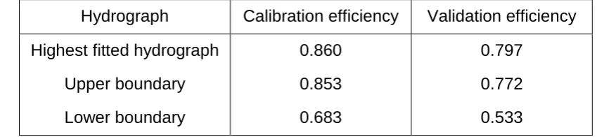
code. Fig. 2 provides an example of the distributions of overland flow parcels 376
from three individual source cells on hillslopes after a time step (6 min) in a 377
modelling run. The source cells of overland flow were selected to 378
demonstrate the algorithm, and overland flow from each source cell is 379
separated into 10000 water parcels, each of which go through the algorithm 380
to determine a location after the current time step in the model. For the cell 381
on the top or middle of hilslopes (e.g. a and c), most parcels stop on the 382
near downstream cells of the source cell after a time step even though there 383
is a wide spread of overland flow parcels. This is because overland flow 384
velocity in these locations is quite slow. It should be noted that the green 385
cells in the figures only represent one to ten parcels (i.e. the magnitude of 386
0.01% - 0.1% of all overland flow from the source cell) so some individual 387
parcels moving to very far downstream positions from the sources can only 388
represent small probability events due to the stochastic algorithm of overland 389
flow routing. The overland flow parcels from the source cell at the bottom of 390
hilslopes (e.g. b) concentrate on cells further from the source cells after a 391
time step, as the flow paths of these parcels are at the bottom of hillslopes 392
and in river channels in which the overland flow velocity is much higher than 393
that on top and middle of hillslopes. 394
395
After running through all cells (from high to low) in the catchment, the 396
overland flow in the outlet cell is the overland flow output of the catchment in 397
the current time step. This flow includes overland flow produced in current 398
time steps in the area near the outlet and in former steps at longer distances 399
away from it. Overland flow in the hillslope cells can lead to overland flow 400
output or be part of subsurface flow output due to re-infiltration. 401
2.2.2 Time delay process and its equations
403
The time delay for water movement on hillslopes is generated by the down-404
flow accumulation of cell to cell delays, estimated from the velocity variations 405
induced by acceleration and friction, which are themselves driven by 406
topographic factors and land surface features. The equations for delay time 407
of overland flow (or the equations for velocity of overland flow) should 408
therefore be related to surface gradient, flow depth, and land surface cover. 409
The Darcy-Weisbach equation (as Equation 23) can be utilized as an 410
expression of land surface resistance to overland flow, which provides a 411
theoretically-based way to build relationships among overland flow velocity, 412
gradient, flow depth and the friction factor in upland peatlands backed up by 413
empirical observations (Holden et al., 2008): 414
415
Equation 23 416
where S is the surface slope and, v is the mean velocity of overland flow, d 417
is overland flow depth, g is gravitational acceleration, and f is the 418
dimensionless friction factor. f can be related to the ratio of water depth, d to 419
an effective roughness diameter, k, which can be described by an empirical 420
equation (Equation 24): 421
422
Equation 24 423
where A is an empirically defined constant. 424
425
Combining Equation 23 and Equation 24, overland flow velocity will be 426
related to flow depth and slope gradient with a couple of constants but the 427
expression may be complex. From the work of Holden et al. (2008), when 428
we have 10 < d/k <10000 there is a relationship of f -0.5~ (d/k)1/6 which is
429
consistent with Manning’s equation. Thus we can simplify to: 430
431
Equation 25 432
where kv is a suitable constant based on Equation 23 and Equation 24. This
433
is a succinct form of a velocity calculation in which water depth will be 434
obtained in every cell at every time step during model runs. Gradient can be 435
2 8g
v dS
f =
1
1.77 ln d
A
k f
= +
2/3 1/ 2 v
gained through an analysis of elevation data before the hydrological 436
simulation. 437
438
The algorithms describing overland flow movement have been presented in 439
this section. The new model therefore has the ability to represent land-cover 440
change impacts on overland flow in a fully distributed fashion. We now test 441
the model for an upland peatland. 442
443
3 Study site
444
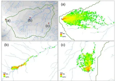
The Trout Beck catchment (54 41’ N, 2 23’ W) is situated at Moor House 445
National Nature Reserve (also a World Biosphere Reserve) in the North 446
Pennine region of northern England, covering an area of 11.4 km2 (see Fig.
447
3). It is one of the headwaters of the River Tees, with an elevation ranging 448
from 842 m to 533 m AOD. Hourly river flow and weather data from 1993 to 449
2009 was obtained for the site. Around 90% of the catchment is covered by 450
blanket peat with a typical depth of 1-2 m (Evans et al., 1999). The peat 451
suffered widespread erosion in the 1950s, but large areas have re-vegetated 452
with Sphagnum and Eriophorum since then (Grayson et al., 2010). A 453
Calluna-Eriophorum association dominates the vegetation cover of the
454
catchment, and in areas above 630 m AOD, Eriophorum alone becomes 455
dominant (Evans et al., 1999). 456
457
The climate of the catchment is classified as sub-arctic oceanic (Manley, 458
1942), with an annual average temperature (1931–2006) of 5.3 °C (Holden 459
and Rose, 2011), and a mean annual rainfall of 2012 mm (records from 460
1951 to 1980 and 1991 to 2006) (Holden and Rose, 2011). 43% of the 461
annual precipitation falls between April to September (Grayson et al., 2010). 462
463
4 Model calibration and validation
464
4.1 Method and model setting 465
The GLUE method of Beven and Binley (1992) rejects the concept of an 466
optimum or best parameter set for a system, and all parameter sets are 467
system. The existence of multiple behavioural parameter sets is a generic 469
modelling problem in the face of uncertainty (Cameron et al., 1999). From a 470
specified parameter space, many parameter sets are picked using Monte 471
Carlo simulation, evaluated by likelihood measures and some are rejected 472
as non-behavioural after the assessment. This framework is now widely 473
used to estimate uncertainty and evaluate results in hydrological modelling 474
(e.g. Freer et al., 1996; Aronica et al., 2002). 475
476
For the distributed TOPMODEL, the number of simulation runs for calibration 477
and validation must be limited, because the distributed model can have a 478
long run time. Thus, the three crucial parameters of m, K, and kv in the
479
distributed TOPMODEL were only taken into account in the test process. m 480
is the active depth for subsurface flow; K is a ‘notional’ hydraulic conductivity 481
of soil in the model (K × m is the transmissivity); kv is the velocity parameter
482
of overland flow. Due to the shortage of field observations of these 483
parameters, they were assumed to be homogeneous throughout the 484
catchment for the purposes of the test. 485
486
The experience from other TOPMODEL applications (Beven, 1997; Kirkby, 487
1997) can be used to narrow the parameter space and so restrict the 488
number of calibration runs needed. In order to avoid uneven distribution of 489
parameter sets in parameter space caused by such a limited number of 490
runs, the parameter sets were scanned systematically in the parameter 491
space (as shown in Table 1), giving 90 sets of parameters for calibration. 492
493
Comparing the simulated hydrographs with the observed one, the Nash-494
Sutcliffe efficiency (the measure of likelihood) of each simulation result was 495
calculated. The top 20% of simulated hydrographs with the highest efficiency 496
are then used to compose an envelope band of hydrographs which is 497
compared to the observed runoff through the calibration period. These top 498
20% parameter sets were picked to run the model through the validation 499
period. The same top 20% of parameter sets were then used to created 500
envelope bands of the validation storm and compared to the observed 501
hydrograph of the validation period. 502
To avoid freezing and melting problems and the lower reliability of winter 504
precipitation records due to snowfall, rainfall events for model calibration and 505
validation were selected from summer-half years (from 1993 to 2009). Fig. 4 506
summarises the yearly maximum hourly summer rainfall. A one-week period 507
commencing from 16th August 2004 (105 mm total rainfall) has been chosen
508
as a suitable period for calibration. It includes a storm event with 19.4 mm 509
precipitation in one hour which represents an approximately 10-year return 510
period estimated from the empirical frequency of events (Fig. 4). Another wet 511
week near to the calibration period is selected as the validation period 512
commencing from 8th August 2004 (128 mm total rainfall). The
Penman-513
Monteith equation is employed to estimate potential evapotranspiration 514
during the calibration and validation periods. It is assumed that actual 515
evapotranspiration is equal to potential evapotranspiration, as peat soil is 516
very wet and there is plentiful water for evapotranspiration in the catchment. 517
518
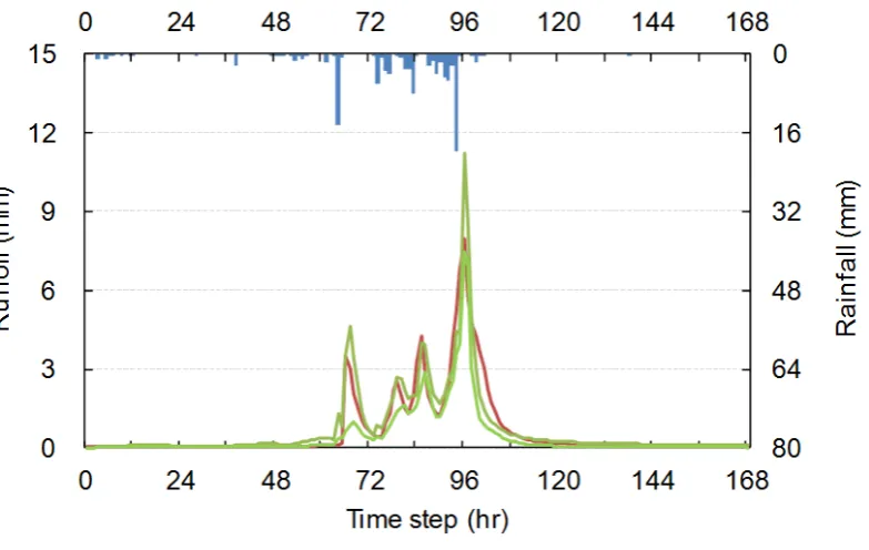
4.2 Results of calibration and validation 519
For the flow calibration, the Nash-Sutcliffe efficiency for each simulation run 520
was computed to measure the likelihood, and the top 20% hydrograph band 521
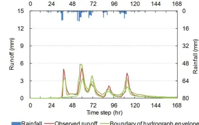
is plotted in Fig. 5. The top 20% of parameter sets in the calibration were run 522
in the model during the validation period and the band of resulting 523
hydrographs is illustrated in Fig. 6. The two hydrograph bands of calibration 524
and validation span most of the observed hydrographs in the two periods. 525
The Nash-Sutcliffe efficiency for the single best-fitted hydrograph, the upper 526
boundary of the band, and the lower boundary of the band were calculated 527
to represent the model performance during both the calibration and 528
validation periods (Table 2). The model performance was satisfactory since 529
the Nash-Sutcliffe efficiency of the top 20% simulations in the calibration is 530
over 0.78, and that in validation is more than 0.64. This test result 531
demonstrates that the distributed TOPMODEL can simulate runoff well for 532
the Trout Beck catchment. 533
534
4.3 Comparison of the distributed TOPMODEL and the original 535
TOPMODEL 536
To compare the distributed TOPMODEL to the original TOPMODEL, the 537
same modified GLUE procedure was applied to the Trout Beck catchment 538
data with the same storm events for calibration and validation, applying the 539
same as those in the distributed TOPMODEL. V is the uniform velocity of 541
runoff. All three parameters are homogenous for the catchment due to the 542
lumped configuration of the original TOPMODEL. Parameter ranges of m 543
and K are kept from the test in the distributed TOPMODEL, and Table 3 544
shows the parameter space for the original TOPMODEL, in which there are 545
90 parameter sets. 546
547
The hydrograph band constituted from the top 20% efficiency results for the 548
calibration runs is illustrated in Fig. 7. Using these top 20% parameter sets 549
the hydrograph band was produced from validation runs (Fig. 8) and Table 4 550
shows the Nash-Sutcliffe efficiency of the hydrograph bands in the 551
calibration and validation. 552
Comparing the test results of the distributed TOPMODEL and the original 553
TOPMODEL, the calibration hydrograph bands are quite similar for the two 554
models. The Nash-Sutcliffe efficiency of the highest fitted hydrograph and 555
the upper boundary in the results of the original TOPMODEL is slightly better 556
than the distributed model. However, for the validation results, the 557
hydrograph band of the distributed TOPMODEL envelopes more parts of the 558
observed hydrograph. The Nash-Sutcliffe efficiency of all three 559
representative curves for the band of the distributed TOPMODEL is distinctly 560
better than that for the original TOPMODEL. The two envelopes in the 561
calibration and validation periods for the distributed TOPMODEL bracket 562
50.0% and 68.5% of the observations respectively (Fig. 5 and Fig. 6), and 563
for the original TOPMODEL they are 37.6% and 42.8% (Fig. 7 and Fig. 8). 564
This comparison implies that the new distributed TOPMODEL performed 565
better than the original version in this catchment, and the distributed 566
configuration and the new overland flow module seem to improve the 567
model’s ability to predict river flow. Clearly this is in addition to the benefits 568
developed including the spatial distribution and the fact that users of the new 569
model can also determine overland flow volumes and velocities across any 570
point in the catchment for each time step used. 571
572
However, the cost of the distributed model is time of model runs. The 573
simulation of the distributed TOPMODEL takes about 20 min per run (a 574
simulation week) using an Intel i7 Processor (4 core 2.0 GHz), while the 575
original one takes less than 2 seconds for a run. In the distributed 576
step mainly depends on the overland flow contributing area which is related 578
to the rainfall amount in the current time step and the overland flow 579
contributing area formed in the previous time steps. A larger contributing 580
area means that more cells are under calculation for the overland flow 581
routing and re-infiltration in the overland flow module, and that, for an 582
individual cell in the contributing area, the overland flow route has a greater 583
chance of being extended. These distributed overland flow calculations are 584
more time-consuming than the subsurface flow calculation. 585
586
In terms of the key parameters used in the two models, the transmissivity 587
(T0) has a large difference between models. The range of transmissivity in
588
the original TOPMODEL is 100 – 300 m2 hr-1 while it is 0.3 – 5.4 m2 hr-1 in
589
the distributed TOPMODEL. As indicated by Wigmosta and Lettenmaier 590
(1999), effective transmissivity values predicted by the original TOPMODEL 591
are higher than the simulated result given by a subsurface flow kinematic 592
wave solution. On the other hand, higher transmissivity leads to more 593
subsurface flow. Around 80% of runoff is subsurface flow in the calibration 594
period in the simulations of the original TOPMODEL, and this proportion of 595
subsurface flow seems to be too high for blanket peatland catchments, in 596
which peak runoff should be dominated by surface or very near-surface flow 597
(Holden and Burt, 2002). However, this situation is different for the 598
distributed TOPMODEL. Only about 20% of runoff is subsurface flow during 599
the calibration period in the simulations of the distributed TOPMODEL. Thus, 600
it may be inferred that the development of the distributed TOPMODEL 601
improves the physical meanings of the model with respect to blanket peat 602
headwaters. 603
604
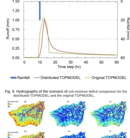
A scenario was employed to demonstrate the difference between simulated 605
soil moisture deficit for the two models. The example shown in Fig. 9 was 606
run for 100 time steps with a rainfall input which consists of a 1-hour storm 607
with 20 mm hr-1 rate at time step 11. A parameter set having high efficiency
608
(over 0.8) in the calibration and validation was chosen to run the distributed 609
TOPMODEL and the same values of K (hydraulic conductivity) and m 610
(scaling parameter) were also used in the original TOPMODEL for 611
comparison. The overland flow velocity parameter (V) of the original 612
TOPMODEL was optimized to match the resulting hydrograph with that of 613
the distributed TOPMODEL. The simulation runs of the two models start with 614
first modelling time step is derived for both runs of the two models. Fig. 9 616
shows the resulting hydrographs of the two models for this scenario. 617
618
At the time step 10 (just before the rainfall input), the values of soil moisture 619
deficit and their spatial distributions for the two models are quite similar (as 620
shown in Fig. 10 (a) and (d)). This is because both of the models applied the 621
same mechanism of subsurface flow simulation even though the distributed 622
structure is adopted in the new model. At the time step just after the rainfall 623
event (time step 12), the soil moisture deficit within the simulation of the 624
distributed TOPMODEL is lower than that within the original TOPMODEL 625
(see Fig. 10 (b) and (e)). Hence there are wetter hillslopes in the distributed 626
TOPMODEL than those in the original one due to the reinfiltration 627
mechanism. After rainfall, the soil moisture deficit of the two simulations both 628
decrease step by step after the storm. Fig. 10 (c) and (f) illustrate that the 629
moisture deficit of the distributed model simulation is still larger than that 630
within the original model at time step 40 but the difference between them is 631
less than that in the earlier time step just after the rainfall. 632
633
From the above scenario modelling, we can show that re-infiltration 634
mechanisms in the distributed TOPMODEL decrease soil moisture deficit 635
after storm events as more surface water infiltrates into soil during the 636
process of overland flow movement on hilslopes. At the same time, overland 637
flow delay on hillslopes in the model provides more ‘opportunities’ to 638
overland flow for re-infiltration. These changes in the distributed 639
TOPMODEL should result in improvements to peak flow modelling. Güntner 640
et al. (1999), compared simulated runoff components from the original
641
TOPMODEL and those derived from hydrograph separation by tracer 642
investigations and field observations during two storm events in a German 643
mountainous forested basin (Brugga basin, 40 km2). The modelled
644
saturation-excess overland flow reached peaks earlier than the real 645
saturation-excess overland flow, and the peak contributions of simulated 646
saturation-excess overland flow were larger than those of measured event 647
water. Their work highlighted a deficiency of the original TOPMODEL but our 648
distributed version of TOPMODEL makes significant improvements through 649
the overland flow delay and re-infiltration mechanisms. The overland flow 650
routing process in the new model provides a reasonable delay of overland 651
flow movement on hillslopes and makes a part of saturation-excess overland 652
the findings of Güntner et al. (1999), in which the exchange between surface 654
and subsurface water and the flow source and path was recommended for 655
future catchment hydrological modelling. 656
657
5 Model sensitivity to land-cover change and future
658
applications
659
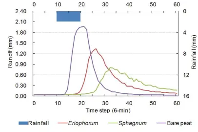
The new model was designed to describe the land cover impact on overland 660
flow movement, so it should be sensitive to varying land cover types. Three 661
scenarios, representing bare peat, Eriophorum cover and Sphagnum cover 662
(which are three typical land cover types in the Trout Beck catchment) 663
respectively covering the whole catchment, were performed as preliminary 664
test of the model sensitivity to land-cover change. The parameter set used in 665
the Eriophorum scenario was picked up in the calibration and validation 666
procedure (the efficiency of the set is over 0.8), in which the land cover was 667
assumed to be uniform over the catchment, as the Trout Beck catchment is 668
primarily dominated by Eriophorum (Evans et al., 1999). The other two 669
scenarios used the same parameters in the set except for the overland flow 670
velocity parameter. Using the empirical research of Holden et al. (2008) the 671
overland flow velocity parameter in bare peat is five times greater than for 672
Eriophorum, while the overland flow velocity parameter in Sphagnum is half
673
that of Eriophorum. A one hour rainfall pulse with a uniform rate of 20 mm hr
-674
1 (i.e. 2 mm per 6-min), which is similar to the one in 10-year summer rainfall
675
event (Fig. 4) was the precipitation input in model runs used for the 676
sensitivity test. The modelling time step was set as 0.1 hr (6 min) to examine 677
differences in flow peak time and magnitude between cover type scenarios. 678
679
The outlet hydrographs of the three scenarios are illustrated in Fig. 11, 680
indicating that there are large differences among the results. If we 681
considered the Eriophorum scenario as a standard, the bare peat scenario 682
produces a 46.3 % higher and a 5-step earlier peak than the Eriophorum 683
scenario while the Sphagnum one gives a 40.3 % lower and 6-step later 684
peak than the standard one. This implies that the model is sensitive to the 685
overland flow velocity parameter which is associated with land cover type. 686
6 Conclusions
688
This paper has developed novel work to transform the traditional 689
TOPMODEL into a distributed differential model, retaining classical key 690
ideas on runoff production but focusing on land-cover change impacts on 691
overland flow velocities leading to river flow hydrographs. The new model is 692
totally distributed with a computational unit of a grid cell. In the new 693
distributed model, the impacts of land-cover change on in-situ water 694
movement and downstream river flow can both be represented and 695
simulated by this model improvement. At the same time, the distributed 696
model has another crucial advantage in that it can represent the spatial 697
variability of precipitation for rainfall-runoff simulations. The spatial variability 698
of rainfall can greatly affect the timing and shape of peak flow hydrographs 699
(Wilson et al., 1979; Syed et al., 2003), no matter which scale of catchment 700
is being investigated (e.g. 4-5 ha. Faures et al., 1995). On the other hand, 701
rainfall variability in space can also produce problems in calibrating 702
hydrological models (Arnaud et al., 2002). Distributed hydrological models 703
allow the distribution pattern of rainfall input to be provided in the model. 704
This means every cell can be assigned rainfall inputs for every time step, 705
which is a disaggregated way to describe the spatial and temporal variability 706
of rainfall. Thus, the model can utilise more accurate precipitation data (e.g. 707
from rainfall radar) to decrease the negative influence of rainfall spatial 708
variability on flow modelling. Of course the availability of distributed rainfall 709
data is a practical problem for many upland sites but it is thought that such 710
data availability will improve over time and thus the model is ready and fit-711
for-purpose for future flow modelling in upland systems. 712
713
A new module, with a series of distributed algorithms representing water 714
routing and velocity, models the movement of overland flow and the surface 715
cover impact on overland flow. After the overland flow routing process, a 716
water parcel stops at a downstream cell in which it is treated as input water 717
for the cell and may infiltrate into the soil to contribute to subsurface flow 718
produced in this cell or it may add to further overland flow production 719
associated with changes in flow depth for the cell for the given time step. 720
This mechanism reflects the real process of overland flow generation on 721
hillslopes and may be influenced by land cover. Land-cover change 722
decreases or increases transportation time for overland flow and thus 723
decreases or increases the opportunity for the infiltration of overland flow. 724
the distributed TOPMODEL is rarely considered in catchment hydrological 726
models. A similar mechanism can only be found in a few hydrological 727
modelling studies such as the work of Wang et al. (2011) by which the 728
mechanism was used in the model for rainfall-runoff simulations for a macro-729
scale (> 10000 km2) catchment with a resolution of 1-km grid cells or rather
730
larger than the hillslope scale overland flow process. At the same time as 731
providing this significant new advance which could have wide applicability, 732
there is only one key parameter (kv the parameter of overland flow velocity)
733
which has been added for overland flow compared to the constant overland 734
flow velocity parameter in the original TOPMODEL, limiting the possibilities 735
of over-parameterization (Perrin et al., 2001). The small number of 736
parameters required to run the model is an obvious benefit for the 737
application of the model, and makes it easier to calibrate and validate in 738
practice. 739
740
The model was found to be very sensitive to land cover type. Therefore it 741
can be used in future studies which test different spatially-distributed 742
scenarios of land-cover change which upland peatland managers are 743
concerned about. These concerns may include removal of vegetation (e.g. 744
by erosion processes, pollution, overgrazing) or good revegetation of peat 745
with sedges such as Eriophorum or mosses such as Sphagnum. It should be 746
possible to conduct experiments with the model to test for optimum 747
locations, concentrations and sizes of land-cover change in order to reduce 748
flood peaks. 749
Acknowledgements
750
We would like to thank the China Scholarship Council and the School of 751
Geography of the University of Leeds for funding this project. We are also 752
grateful to the UK’s Environmental Change Network for provision of data. 753
754
References
755
756
Arnaud P, Bouvier C, Cisneros L, Dominguez R. 2002. Influence of rainfall 757
spatial variability on flood prediction. Journal of Hydrology, 260: 216-758
Aronica G, Bates PD, Horritt MS. 2002. Assessing the uncertainty in 760
distributed model predictions using observed binary pattern 761
information within GLUE. Hydrological Processes, 16: 2001-2016. 762
DOI: 10.1002/hyp.398. 763
Ballard CE, McIntyre N, Wheater HS, Holden J, Wallage ZE. 2011. 764
Hydrological modelling of drained blanket peatland. Journal of 765
Hydrology, 407: 81-93. DOI: 10.1016/j.jhydrol.2011.07.005. 766
Beven K. 1997. TOPMODEL: A critique. Hydrological Processes, 11: 1069-767
1085. DOI: 10.1002/(sici)1099-1085(199707)11:9<1069::aid-768
hyp545>3.0.co;2-o. 769
Beven K, Binley A. 1992. The future of distributed models - model calibration 770
and uncertainty prediction. Hydrological Processes, 6: 279-298. DOI: 771
10.1002/hyp.3360060305. 772
Beven KJ, Kirkby MJ. 1979. A physically-based variable contributing area 773
model of basin hydrology. Hydrological Sciences Bulletin, 24: 43-69. 774
Beven KJ, Kirkby MJ, Schofield N, Tagg AF. 1984. Testing a physically-775
based flood forecasting-model (Topmodel) for 3 UK catchments. 776
Journal of Hydrology, 69: 119-143. DOI: 10.1016/0022-777
1694(84)90159-8. 778
Bower MM. 1962. The cause of erosion in blanket peat bogs. Scottish 779
Geographical Magazine, 78: 33-43. 780
Bragg OM, Tallis JH. 2001. The sensitivity of peat-covered upland 781
landscapes. Catena, 42: 345-360. DOI: 10.1016/s0341-782
8162(00)00146-6. 783
Cameron DS, Beven KJ, Tawn J, Blazkova S, Naden P. 1999. Flood 784
frequency estimation by continuous simulation for a gauged upland 785
catchment (with uncertainty). Journal of Hydrology, 219: 169-187. 786
DOI: 10.1016/s0022-1694(99)00057-8. 787
Evans MG, Burt TP, Holden J, Adamson JK. 1999. Runoff generation and 788
water table fluctuations in blanket peat: evidence from UK data 789
spanning the dry summer of 1995. Journal of Hydrology, 221: 141-790
160. DOI: 10.1016/s0022-1694(99)00085-2. 791
Evans R. 2005. Curtailing grazing-induced erosion in a small catchment and 792
its environs, the Peak District, Central England. Applied Geography, 793
25: 81-95. DOI: 10.1016/j.apgeog.2004.11.002. 794
Faures JM, Goodrich DC, Woolhiser DA, Sorooshian S. 1995. Impact of 795
small-scale spatial rainfall variability on runoff modeling. Journal of 796
Hydrology, 173: 309-326. DOI: 10.1016/0022-1694(95)02704-s. 797
Franks SW, Gineste P, Beven KJ, Merot P. 1998. On constraining the 798
predictions of a distributed moder: The incorporation of fuzzy 799
estimates of saturated areas into the calibration process. Water 800
Resources Research, 34: 787-797. DOI: 10.1029/97wr03041. 801
Freer J, Beven K, Ambroise B. 1996. Bayesian estimation of uncertainty in 802
runoff prediction and the value of data: An application of the GLUE 803
approach. Water Resources Research, 32: 2161-2173. DOI: 804
10.1029/95wr03723. 805
Güntner A, Uhlenbrook S, Seibert J, Leibundgut C. 1999. Multi-criterial 806
validation of TOPMODEL in a mountainous catchment. Hydrological 807
Gallego-Sala AV, Prentice IC. 2013. Blanket peat biome endangered by 809
climate change. Nature Climate Change, 3: 152-155. DOI: 810
10.1038/nclimate1672. 811
Grayson R, Holden J, Rose R. 2010. Long-term change in storm 812
hydrographs in response to peatland vegetation change. Journal of 813
Hydrology, 389: 336-343. DOI: 10.1016/j.jhydrol.2010.06.012. 814
Hess TM, Holman IP, Rose SC, Rosolova Z, Parrott A. 2010. Estimating the 815
impact of rural land management changes on catchment runoff 816
generation in England and Wales. Hydrological Processes, 24: 1357-817
1368. DOI: 10.1002/hyp.7598. 818
Hoare CAR. 1962. Quicksort. Computer Journal, 5: 10-16. DOI: 819
10.1093/comjnl/5.1.10. 820
Holden J. 2005. Peatland hydrology and carbon release: why small-scale 821
process matters. Philosophical Transactions of the Royal Society a-822
Mathematical Physical and Engineering Sciences, 363: 2891-2913. 823
DOI: 10.1098/rsta.2005.1671. 824
Holden J, Burt TP. 2002. Infiltration, runoff and sediment production in 825
blanket peat catchments: implications of field rainfall simulation 826
experiments. Hydrological Processes, 16: 2537-2557. DOI: 827
10.1002/hyp.1014. 828
Holden J, Burt TP. 2003. Runoff production in blanket peat covered 829
catchments. Water Resources Research, 39. DOI: 830
10.1029/2002wr001956. 831
Holden J, Chapman PJ, Labadz JC. 2004. Artificial drainage of peatlands: 832
hydrological and hydrochemical process and wetland restoration. 833
Progress in Physical Geography, 28: 95-123. DOI: 834
10.1191/0309133304pp403ra. 835
Holden J, Kirkby MJ, Lane SN, Milledge DG, Brookes CJ, Holden V, 836
McDonald AT. 2008. Overland flow velocity and roughness properties 837
in peatlands. Water Resources Research, 44. DOI: 838
10.1029/2007wr006052. 839
Holden J, Rose R. 2011. Temperature and surface lapse rate change: a 840
study of the UK's longest upland instrumental record. International 841
Journal of Climatology, 31: 907-919. DOI: 10.1002/joc.2136. 842
Holden J, Shotbolt L, Bonn A, Burt TP, Chapman PJ, Dougill AJ, Fraser 843
EDG, Hubacek K, Irvine B, Kirkby MJ, Reed MS, Prell C, Stagl S, 844
Stringer LC, Turner A, Worrall F. 2007b. Environmental change in 845
moorland landscapes. Earth-Science Reviews, 82: 75-100. DOI: 846
10.1016/j.earscirev.2007.01.003. 847
Immirzi CP, Maltby E, Clymo RS. 1992. The global status of peatlands and 848
their role in carbon cycling. In: A report for Friends of the Earth by the 849
Wetland Ecosystems Research Group, Dept Geography, University of 850
Exeter, pp: 1-145. 851
IUCN. 2011. IUCN UK Commission of Inquiry on Peatlands. In: IUCN UK 852
Peatland Programme. 853
Kirkby MJ. 1976. Chapter 3 Hydrograph modelling strategies. In: Processes 854
in Physical and Human Geography, Peel R, Chisholm M, Haggett P 855
(eds.) Heinemann. 856
Kirkby MJ. 1997. TOPMODEL: A personal view. Hydrological Processes, 11: 857
1087-1097. DOI: 10.1002/(sici)1099-1085(199707)11:9<1087::aid-858
Lamb R, Beven K, Myrabo S. 1998. Use of spatially distributed water table 860
observations to constrain uncertainty in a rainfall-runoff model. 861
Advances in Water Resources, 22: 305-317. DOI: 10.1016/s0309-862
1708(98)00020-7. 863
Lane SN, Milledge DG. 2013. Impacts of upland open drains upon runoff 864
generation: a numerical assessment of catchment-scale impacts. 865
Hydrological Processes, 27: 1701-1726. DOI: 10.1002/hyp.9285. 866
Manley G. 1942. Meteorological observations on Dun Fell, a mountain 867
station in northern England. Quarterly Journal of the Royal 868
Meteorological Society, 68: 151-165. 869
O'Callaghan JF, Mark DM. 1984. The extraction of drainage networks from 870
digital elevation data. Computer Vision Graphics and Image 871
Processing, 28: 323-344. DOI: 10.1016/s0734-189x(84)80011-0. 872
Parrott A, Brooks W, Harmar O, Pygott K. 2009. Role of rural land use 873
management in flood and coastal risk management. Journal of Flood 874
Risk Management, 2: 272-284. DOI: 10.1111/j.1753-875
318X.2009.01044.x. 876
Parry LE, Holden J, Chapman PJ. 2014. Restoration of blanket peatlands. 877
Journal of Environmental Management, 133: 193-205. 878
DOI: http://dx.doi.org/10.1016/j.jenvman.2013.11.033. 879
Perrin C, Michel C, Andreassian V. 2001. Does a large number of 880
parameters enhance model performance? Comparative assessment 881
of common catchment model structures on 429 catchments. Journal 882
of Hydrology, 242: 275-301. DOI: 10.1016/s0022-1694(00)00393-0. 883
Peters NE, Freer J, Beven K. 2003. Modelling hydrologic responses in a 884
small forested catchment (Panola Mountain, Georgia, USA): a 885
comparison of the original and a new dynamic TOPMODEL. 886
Hydrological Processes, 17: 345-362. DOI: 10.1002/hyp.1128. 887
Price JS. 1992. Blanket bog in Newfoundland. Part 2. Hydrological 888
processes. Journal of Hydrology, 135: 103-119. DOI: 10.1016/0022-889
1694(92)90083-8. 890
Quinn P, Beven K, Chevallier P, Planchon O. 1991. The prediction of 891
hillslope flow paths for distributed hydrological modeling using digital 892
terrain models. Hydrological Processes, 5: 59-79. DOI: 893
10.1002/hyp.3360050106. 894
Sedgewick R. 1978. Implementing quicksort programs. Communications of 895
the Acm, 21: 847-857. DOI: 10.1145/359619.359631. 896
Syed KH, Goodrich DC, Myers DE, Sorooshian S. 2003. Spatial 897
characteristics of thunderstorm rainfall fields and their relation to 898
runoff. Journal of Hydrology, 271: 1-21. DOI: 10.1016/s0022-899
1694(02)00311-6. 900
Wang JH, Yang H, Li L, Gourley JJ, Sadiq IK, Yilmaz KK, Adler RF, Policelli 901
FS, Habib S, Irwn D, Limaye AS, Korme T, Okello L. 2011. The 902
coupled routing and excess storage (CREST) distributed hydrological 903
model. Hydrological Sciences Journal-Journal Des Sciences 904
Hydrologiques, 56: 84-98. DOI: 10.1080/02626667.2010.543087. 905
Wheater H, Evans E. 2009. Land use, water management and future flood 906
risk. Land Use Policy, 26: S251-S264. DOI: 907
Wigmosta MS, Lettenmaier DP. 1999. A comparison of simplified methods 909
for routing topographically driven subsurface flow. Water Resources 910
Research, 35: 255-264. DOI: 10.1029/1998wr900017. 911
Wilson CB, Valdes JB, Rodriguez-Iturbe I. 1979. Influence of the spatial-912
distribution of rainfall on storm runoff. Water Resources Research, 15: 913
321-328. DOI: 10.1029/WR015i002p00321. 914
915
Tables
917
918
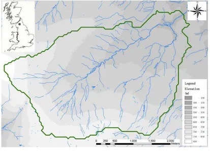
Table 1. Parameter space for the model calibration. 919
920
921
Table 2. Nash-Sutcliffe efficiency of the hydrograph band in the calibration 922
and validation 923
924
925
Table 3. Parameter space for the calibration of the original TOPMODEL. 926
927
928
929
Parameter
Parameter ranges
Lower value Upper value Increment
m (m)
kv
K ( m hr-1)
0.003
10
100
0.018
50
300
0.003
10
100
Hydrograph Calibration efficiency Validation efficiency
Highest fitted hydrograph
Upper boundary
Lower boundary
0.851
0.833
0.785
0.833
0.778
0.644
Parameter
Parameter ranges
Lower value Upper value Increment
m (m)
V (m hr-1)
T0 (m2 hr-1)
0.003
800
100
0.018
1600
300
0.003
200
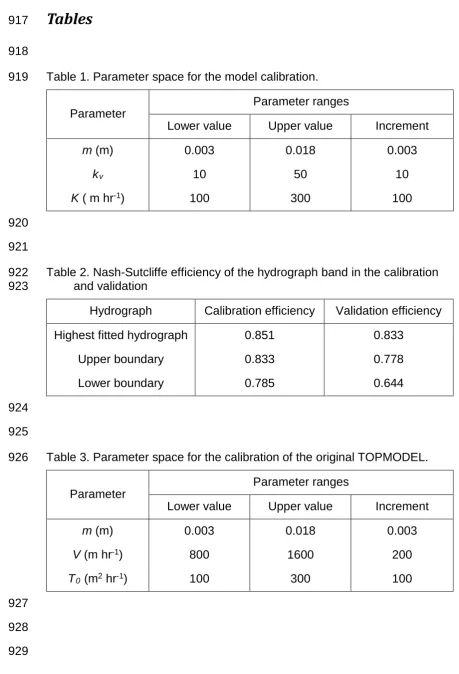
Table 4. Nash-Sutcliffe efficiency of the hydrograph band in the calibration 930
and validation for the original TOPMODEL. 931
Hydrograph Calibration efficiency Validation efficiency
Highest fitted hydrograph
Upper boundary
Lower boundary
0.860
0.853
0.683
0.797
0.772
0.533
Figure list
933
934
Fig. 1. Definition sketch for flow strip (after Kirkby, 1997). x is horizontal 935
distance. 936
937
[image:30.595.127.522.309.588.2]938
Fig. 2. The distributions of water parcels from three individual source cells 939
(a, b and c) on hillslopes after a time step. (The scale of overland flow 940
percentage in the legend is logarithmic). 941
943
Fig. 3. Location and map of the Trout Beck catchment. 944
945
946
Fig. 4. Observed frequency of hourly rainfall intensities of yearly maximum 947
from 1993 to 2009. 948
[image:31.595.120.534.71.374.2]950
Fig. 5. Comparison of the observed runoff and the top 20% simulation 951
hydrograph band in the calibration period. 952
953
[image:32.595.92.521.411.694.2]954
Fig. 6. Comparison of the observed runoff and the hydrograph band in the 955
validation period. 956