University of South Florida
Scholar Commons
Graduate Theses and Dissertations Graduate School
4-5-2017
Extending the Model with Internal Restrictions on
Item Difficulty (MIRID) to Study Differential Item
Functioning
Yong "Isaac" Li
University of South Florida, [email protected]
Follow this and additional works at:http://scholarcommons.usf.edu/etd
Part of theEducational Assessment, Evaluation, and Research Commons, and theEducational Psychology Commons
This Dissertation is brought to you for free and open access by the Graduate School at Scholar Commons. It has been accepted for inclusion in Graduate Theses and Dissertations by an authorized administrator of Scholar Commons. For more information, please contact
Scholar Commons Citation
Li, Yong "Isaac", "Extending the Model with Internal Restrictions on Item Difficulty (MIRID) to Study Differential Item Functioning" (2017).Graduate Theses and Dissertations.
Extending the Model with Internal Restrictions on Item Difficulty (MIRID) to Study Differential Item Functioning
by
Yong “Isaac” Li
A dissertation submitted in partial fulfillment of the requirements for the degree of
Doctor of Philosophy
in Curriculum and Instruction with an emphasis in Educational Measurement and Research Department of Educational and Psychological Studies
College of Education University of South Florida
Co-Major Professor: Yi-Hsin Chen, Ph.D. Co-Major Professor: Jeffrey D. Kromrey, Ph.D.
John Ferron, Ph.D. Stephen Stark, Ph.D.
Date of Approval: March 9, 2017
Keywords: differential item functioning, validity, item response modeling, Rasch models, the MIRID
DEDICATION
ACKNOWLEDGEMENTS
I wish to express my most profound gratitude to my co-major professor, Dr. Yi-Hsin Chen, who brought me into the beautiful world of cognitive diagnostic models and componential IRT modeling. Through his limitless patience and generosity, he guided me along the way of academic pursuit. Whenever I was lost or felt hopeless, he was there and ready to lend me a hand. Without his wisdom, insightful teaching, encouragement, and conviction, I would not have been able to come this far. It has been a pleasant and inspiring experience for me to learn from him and collaborate with him.
I reserve my special thanks and appreciation for my co-major professor, Dr. Jeffrey Kromrey. The epitome of erudition and calmness for people around, I have massive regret for not having been able to learn more from him. But I wish to thank him for steering my research in the right course and granting me important opportunities to gain experience in research. In particular, I am grateful for him to spend valuable hours reviewing and advising my manuscripts and computer code time and again.
My committee members, Dr. John Ferron and Dr. Stephen Stark, have given this study their time and scholarly contributions. I am extremely thankful for their thoughtful suggestions and careful review that have improved the quality of my research. At key moments of this journey, they both provided important, brilliant directions which are characteristic of their academic excellence.
Also, I am indebted to the Research Computing staff at USF, Dr. John Desantis, Dr. Anthony Green, and Joseph Botto, for their tireless assistance and trouble-shooting with regards to my usage of the computing cluster.
Last but not least, I thank my wife, Tina, and daughter, Anwyn, for their patience, understanding, and suffering in these years.
i
TABLE OF CONTENTS
LIST OF TABLES ... iii
LIST OF FIGURES ... v
ABSTRACT ... viii
CHAPTER ONE INTRODUCTION ... 1
Differential Item Functioning in the Context of the MIRID ... 1
DIF as the Consequence of Construct Multidimensionality ... 4
Purpose of the Study ... 6
Significance of the Study ... 9
Definitions... 10
CHAPTER TWO LITERATURE REVIEW ... 13
The Generalized Linear Mixed Models ... 14
The Linear Regression Model ... 14
Linear Mixed Models ... 15
Generalized Linear Models ... 16
Generalized Linear Mixed Models (GLMMs) ... 17
Nonlinear Mixed Models (NLMMs) ... 20
Item Response Modeling in the GLMMs Framework ... 20
The Model with Internal Restrictions on Item Difficulty (MIRID) ... 25
MIRID in the Generalized Statistical Models Framework ... 25
Estimation Methods and Computer Programs for the MIRID ... 35
Differential Item Functioning ... 40
The Mantel-Haenszel Procedure ... 42
Simultaneous Item Bias Test (SIBTEST) ... 42
The Model-based DIF Approach for the MIRID ... 43
Individual-item Level Model Specification (DIF) ... 43
Item-group Level Models (DFFm and DFFc) ... 45
Component Weight Model (DWF) ... 46
CHAPTER THREE METHOD ... 48
Design of the Research ... 48
The Scope... 48
ii Implementation ... 55 Data Generation ... 55 Estimation ... 58 Analysis Procedures ... 60 Evaluation Procedures ... 61
CHAPTER FOUR RESULTS ... 65
Parameter Recovery of the Standard MIRID ... 65
Results for the Proposed Differential Functioning Models ... 66
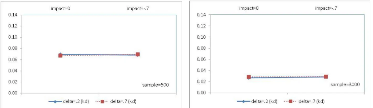
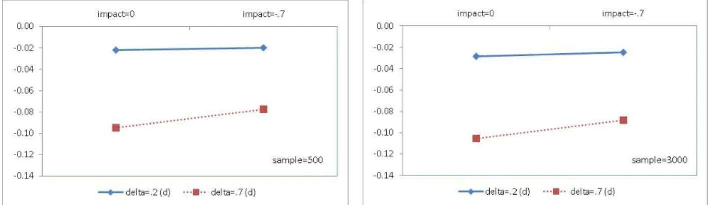
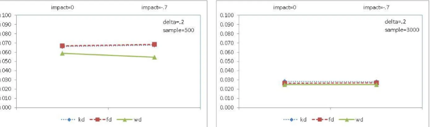
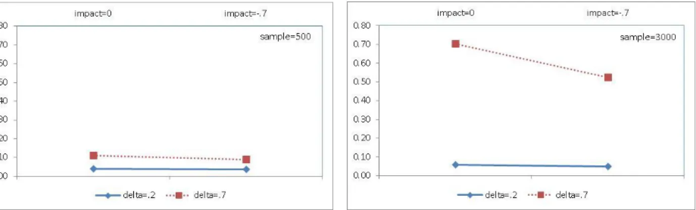
Recovery of the True DIF (Delta) Parameters ... 67
Recovery of Zero-value DIF Parameters ... 75
Type I Error Control and Power of the MIRID Differential Functioning Models ... 80
Results from Fitting the Mismatched Differential Functioning Models ... 96
False Detection Rates of the Mismatched MIRID Differential Functioning Models ... 97
Non-DIF Parameter Recovery of the Mismatched Models ... 113
CHAPTER FIVE DISCUSSION ... 137
Summary ... 137
Findings... 138
Item-Level DIF ... 139
Group-Level DIF ... 141
Mismatching DIF Model and DIF Source ... 142
Implications... 143
Implications for Content Researchers ... 144
Implications for Methodology Researchers ... 146
Limitations and Future Studies ... 148
Conclusions ... 150
REFERENCES ... 151
APPENDIX A: Examples of Analysis Code in SAS ... 161
APPENDIX B: Estimation Bias and RMSEs of the Zero-value DIF Parameters of the MIRID DIF, DFFc, DFFm, and DWF Models ... 163
APPENDIX C: Estimation Bias and rmses of the Model Parameters of the MIRID DFFc, DFFm, and DWF Models ... 165
APPENDIX D: Type I Error Rates and Power Obtained from Estimating Item DIF Parameters by Component and by Item ... 169
iii LIST OF TABLES
Table 1. Item Families and Component Items ... 29
Table 2. Item Predictor Matrix ... 29
Table 3. Component weight Matrix for One Item Family ... 30
Table 4. Parameter Estimates from the Example Study ... 34
Table 5. Simulation Conditions ... 56
Table 6. Recovery of Item Location Parameters of the Standard MIRID ... 68
Table 7 Bias of the Non-zero DIF Parameter Estimates under the MIRID DIF Model ... 69
Table 8. RMSEs of the Non-zero Delta Parameter Estimates under the MIRID DIF Model ... 70
Table 9. Bias of the DIF-related Item Location Parameters under the MIRID DIF ... 72
Table 10 RMSE of the Delta Parameters under the MIRID DFFc, DFFm, and DWF Models ... 74
Table 11 Bias of the Delta Parameters under the MIRID DFFc, DFFm, and DWF Models ... 75
Table 12 Type I Error Rates for MIRID DIF over 500 Replications ... 83
Table 13 Power of the MIRID DIF over 500 Replications ... 85
Table 14 Type I Error Rates for the MIRID DFFc over 500 Replications ... 86
Table 15 Power of the MIRID DFFc over 500 Replications ... 88
Table 16 Type I Error Rates for the MIRID DFFm Model over 500 Replications ... 89
Table 17 Power of the MIRID DFFm over 500 Replications ... 91
Table 18 Type I Error Rates for the MIRID DWF over 500 Replications ... 92
iv
Table 20 Hypothesiswise Type I Error Rates for the Four Proposed MIRID Models ... 95 Table 21 Experimentwise Type I Error Rates after Hochberg Adjustment for the Four Proposed
MIRID Models ... 95 Table 22 False Detection Rates when the MIRID DIF Model Was Applied to the DFFc Data . 101 Table 23 False Detection Rates when the MIRID DIF Model Was Applied to the DFFm Data 102 Table 24 False Detection Rates when the MIRID DIF Model Was Applied to the DWF Data . 103 Table 25 False Detection Rates when the MIRID DFFc Model Was Applied to the DIF Data . 106 Table 26 False Detection Rates when the MIRID DFFc Model Was Applied to the DFFm Data
... 107 Table 27 False Detection Rates when the MIRID DFFc Model Was Applied to the DWF Data
... 108 Table 28 False Detection Rates when the MIRID DFFm Model Was Applied to the DIF Data
... 111 Table 29 False Detection Rates when the MIRID DFFm Model Was Applied to the DFFc Data
... 112 Table 30 False Detection Rates when the MIRID DFFm Model Was Applied to the DWF Data
... 113 Table 31 False Detection Rates when the MIRID DWF Model Was Applied to the DIF Data 116 Table 32 False Detection Rates when the MIRID DWF Model Was Applied to the DFFc Data
... 117 Table 33 False Detection Rates when the MIRID DWF Model Was Applied to the DFFm Data
v LIST OF FIGURES
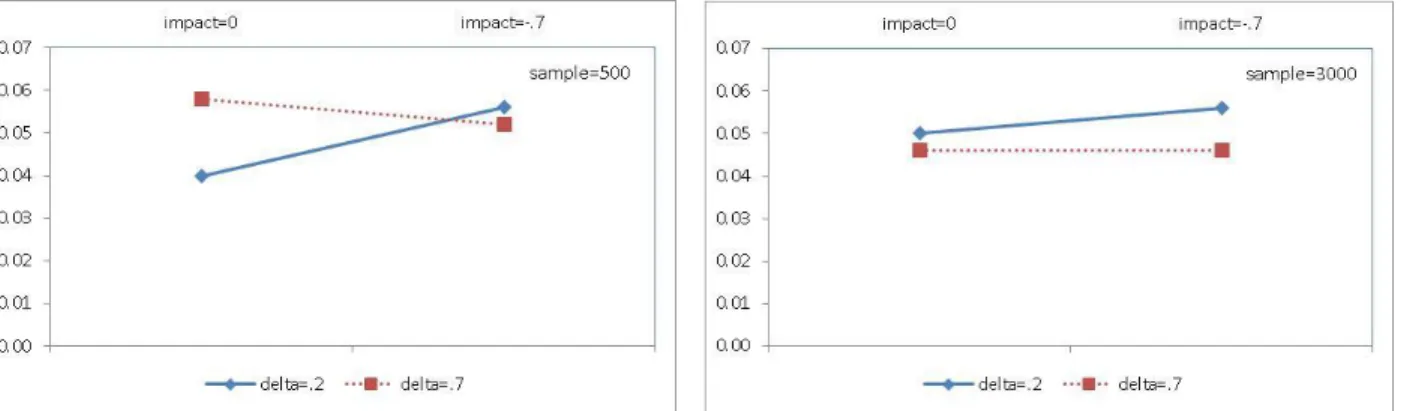
Figure 1. Average bias of the non-zero DIF parameter estimates under the MIRID DIF model by sample size ... 69 Figure 2. Average RMSEs of the non-zero DIF parameter estimates under the MIRID DIF model by sample size ... 70 Figure 3. Recovery of the location parameter of component items under the MIRID DIF model
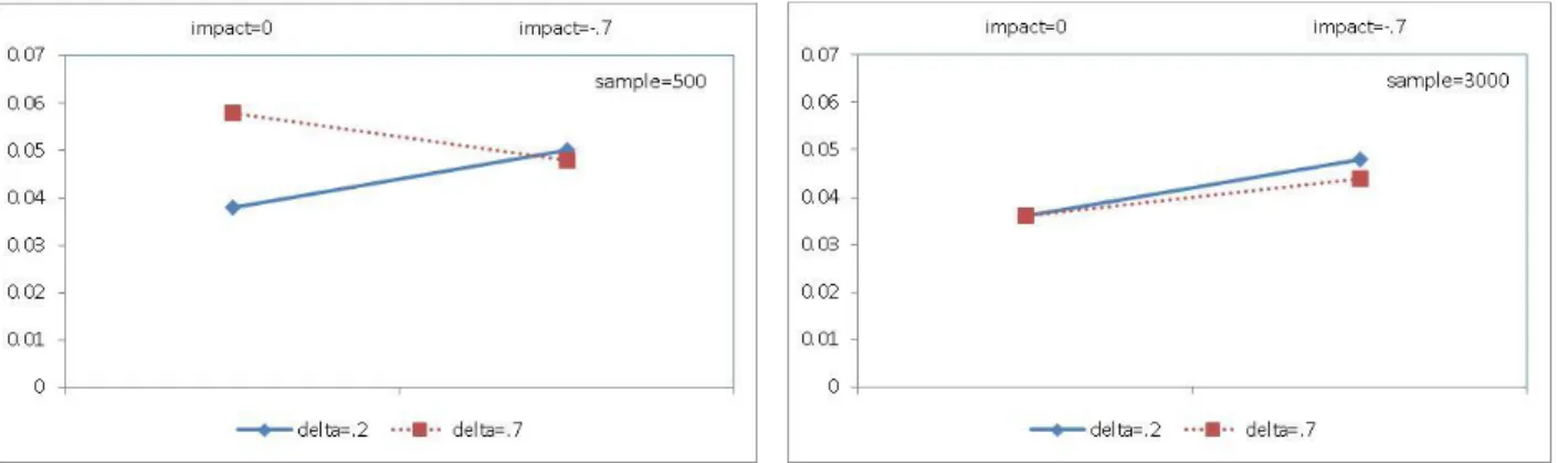
by sample and impact ... 73 Figure 4. RMSEs of the non-zero DIF parameter estimates under the MIRID DFFc by sample
size ... 76 Figure 5. Average RMSEs of the non-zero DIF parameter estimates under the MIRID DFFm by
sample size ... 76 Figure 6. RMSEs of the non-zero DIF parameter estimates under the MIRID DWF by sample
size ... 76 Figure 7. Average bias in estimation of zero-value DIF parameters in the MIRID DIF model ... 77 Figure 8. Average RMSEs in estimation of zero-value DIF parameters in the MIRID DIF model
... 77 Figure 9. Average bias in estimation of zero-value DIF parameters in the MIRID DFFc, DFFm,
and DWF models (smaller delta conditions) ... 78 Figure 10. Average bias in estimation of zero-value DIF parameters in the MIRID DFFc, DFFm, and DWF models (larger delta conditions) ... 78 Figure 11. Average RMSEs in estimation of zero-value DIF parameters in the MIRID DFFc,
DFFm, and DWF models (smaller delta conditions) ... 79 Figure 12. Average RMSEs in estimation of zero-value DIF parameters in the MIRID DFFc,
DFFm, and DWF models (larger delta conditions) ... 79 Figure 13.The MIRID DIF model experiment-wise Type I error rates after Hochberg adjustment
vi
Figure 14. The MIRID DFFc model experimentwise Type I error rates after Hochberg
adjustment by sample size ... 87 Figure 15. The MIRID DFFm model experimentwise Type I error rates after Hochberg
adjustment by sample size ... 90 Figure 16. The MIRID DWF model experimentwise Type I error rates after Hochberg
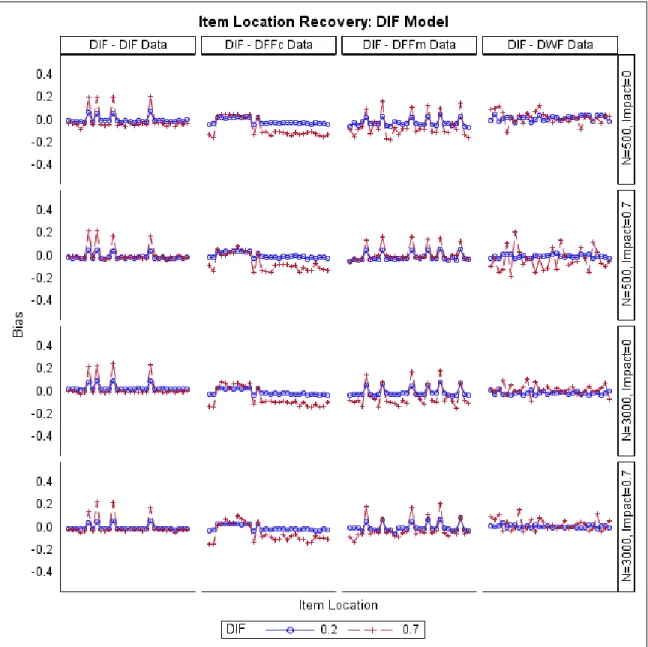
adjustment by sample size ... 93 Figure 17. Bias of the 30 estimated DIF parameters of the MIRID DIF model when fitted to data
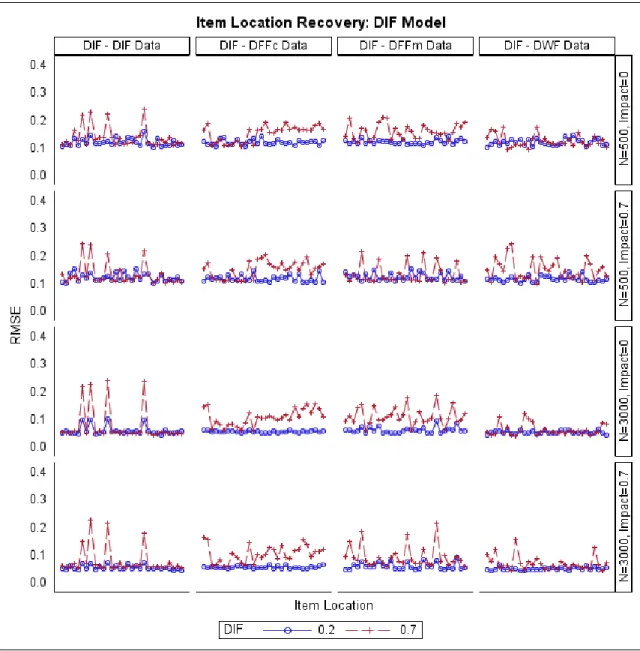
with different sources of differential functioning ... 99 Figure 18. RMSE of the 30 estimated DIF parameters of the MIRID DIF model when fitted to
data with different sources of differential functioning... 100 Figure 19. Bias of the three estimated DIF parameters of the MIRID DFFc model when fitted to
data with different sources of differential functioning... 104 Figure 20. RMSE of the three estimated DIF parameters of the MIRID DFFc model when fitted
to data with different sources of differential functioning ... 105 Figure 21. Bias of the ten estimated DIF parameters of the MIRID DFFm model when fitted to
data with different sources of differential functioning... 109 Figure 22. RMSE of the ten estimated DIF parameters of the MIRID DFFm model when fitted to data with different sources of differential functioning... 110 Figure 23. Bias of the three estimated DIF parameters of the MIRID DWF model when fitted to
data with different sources of differential functioning... 114 Figure 24. RMSE of the three estimated DIF parameters of the MIRID DWF model when fitted
to data with different sources of differential functioning ... 115 Figure 25. Bias of the Estimated Item Locations when the DIF Model Was Fitted to Different
Models ... 119 Figure 26. RMSE of the Estimated Item Locations when the DIF Model Was Fitted to Different
Models ... 120 Figure 27. Bias of the Estimated Item Locations when the DFFc Model Was Fitted to Different
Models ... 121 Figure 28. RMSE of the Estimated Item Locations when the DFFc Model Was Fitted to Different
vii
Figure 29. Bias of the Estimated Item Locations when the DFFm Model Was Fitted to Different Models ... 123 Figure 30. RMSE of the Estimated Item Locations when the DFFm Model Was Fitted to
Different Models ... 124 Figure 31. Bias of the Estimated Item Locations when the DWF Model Was Fitted to Different
Models ... 125 Figure 32. RMSE of the Estimated Item Locations when the DWF Model Was Fitted to Different
Models ... 126 Figure 33. Bias of the Estimated Component Weights when the DIF Model Was Fitted to
Different Models ... 128 Figure 34. RMSE of the Estimated Component Weights when the DIF Model Was Fitted to
Different Models ... 129 Figure 35. Bias of the Estimated Component Weights when the DFFc Model Was Fitted to
Different Models ... 130 Figure 36. RMSE of the Estimated Component Weights when the DFFc Model Was Fitted to
Different Models ... 131 Figure 37. Bias of the Estimated Component Weights when the DFFm Model Was Fitted to
Different Models ... 132 Figure 38. RMSE of the Estimated Component Weights when the DFFm Model Was Fitted to
Different Models ... 133 Figure 39. Bias of the Estimated Component Weights when the DWF Model Was Fitted to
Different Models ... 134 Figure 40. RMSE of the Estimated Component Weights when the DWF Model Was Fitted to
viii ABSTRACT
Differential item functioning (DIF) is a psychometric issue routinely considered in educational and psychological assessment. However, it has not been studied in the context of a recently developed componential statistical model, the model with internal restrictions on item difficulty (MIRID; Butter, De Boeck, & Verhelst, 1998). Because the MIRID requires test questions measuring either single or multiple cognitive processes, it creates a complex
environment for which traditional DIF methods may be inappropriate. This dissertation sought to extend the MIRID framework to detect DIF at the item-group level and the individual-item level. Such a model-based approach can increase the interpretability of DIF statistics by focusing on item characteristics as potential sources of DIF. In particular, group-level DIF may reveal comparative group strengths in certain secondary constructs. A simulation study was conducted to examine under different conditions parameter recovery, Type I error rates, and power of the proposed approach. Factors manipulated included sample size, magnitude of DIF, distributional characteristics of the groups, and the MIRID DIF models corresponding to discrete sources of differential functioning. The impact of studying DIF using wrong models was investigated.
The results from the recovery study of the MIRID DIF model indicate that the four delta (i.e., non-zero value DIF) parameters were underestimated whereas item locations of the four associated items were overestimated. Bias and RMSE were significantly greater when delta was larger; larger sample size reduced RMSE substantially while the effects from the impact factor were neither strong nor consistent. Hypothesiswise and adjusted experimentwise Type I error
ix
rates were controlled in smaller delta conditions but not in larger delta conditions as estimates of zero-value DIF parameters were significantly different from zero. Detection power of the DIF model was weak. Estimates of the delta parameters of the three group-level DIF models, the MIRID differential functioning in components (DFFc), the MIRID differential functioning in item families (DFFm), and the MIRID differential functioning in component weights (DFW), were acceptable in general. They had good hypothesiswise and adjusted experimentwise Type I error control across all conditions and overall achieved excellent detection power.
When fitting the proposed models to mismatched data, the false detection rates were mostly beyond the Bradley criterion because the zero-value DIF parameters in the mismatched model were not estimated adequately, especially in larger delta conditions. Recovery of item locations and component weights was also not adequate in larger delta conditions. Estimation of these parameters was more or less affected adversely by the DIF effect simulated in the
mismatched data. To study DIF in MIRID data using the model-based approach, therefore, more research is necessary to determine the appropriate procedure or model to implement, especially for item-level differential functioning.
1 CHAPTER ONE INTRODUCTION
Modeling cognitive or behavioral constructs underlying item responses with decomposed processes has become an actively researched area in educational and psychological measurement. Different from the traditional practice of trait organization, such componential approaches
recognize intermediate item responses that represent processes as well as the final responses and aim to explain final responses with properties of the intermediate responses. Observations on the “components” supply additional information on more dimensions than can be obtained by focusing on the trait alone. A prominent componential approach, the linear logistic test model (LLTM; Fischer, 1973, 1977), has been adopted by practitioners from many disciplines and served as the platform for development of newer psychometric models, such as the model with internal restrictions on item difficulty (MIRID; Butter, De Boeck, & Verhelst, 1998). Originally a member of the Rasch family of models, the MIRID has had many extensions which provide a new context for investigating measurement issues common to education and psychology. This dissertation concentrated on one of them, differential item functioning (DIF).
Differential Item Functioning in the Context of the MIRID
At the heart of test fairness and construct validity is the issue of differential item functioning, which has received extensive research in the past decades. A general definition provided by Chang, Mazzeo, & Roussos (1996) considers an item as having DIF when conditional on the latent trait being measured, one group of respondents having on average
2
higher probability than the other group to give a particular response to the item. Commonly seen in the literature are DIF analyses to answer the question whether particular items became unfairly easier for members of the focal group than for the reference group.
Numerous procedures have been devised and implemented for DIF detection. Among the most often used are the Mantel-Haenszel (MH) (Holland & Thayer, 1988) method, which is non-parametric, and several model-based procedures, such as Lord's chi-square method (Lord, 1980), Raju's (1990) area measures, and the likelihood ratio test (Thissen, Steinberg, & Wainer, 1993). These procedures have been proven successful in discovering DIF but not as much in helping to understand its possible causes. Moreover, it is unclear the extent to which these traditional approaches are effective when faced with the unique characteristics of the MIRID.
A confirmative approach to examine how underlying processes affect a complex behavioral outcome, the MIRID assumes that the construct of interest can be decomposed into mental processes represented by different items and that there is a definitive between-item relationship similar to that of the LLTM with disparate groups of items retaining one or more properties. For example, performance on questions of addition, subtraction, and multiplication are expected to influence response to items subsuming all these operations. Tests designed in the framework of the MIRID are made of a number of item families, each of which consists of one or more component items measuring individual processes (subtasks) as well as a composite item requiring all these subtasks to answer. Every item family corresponds to a “situation” describing the construct and shares the same number of component items. The difficulty parameter of the composite item is defined as weighted summation of the parameters of all component items in this family plus an intercept. In other words, the MIRID assumes that the difficulty of a
3
composite item is explained perfectly by the difficulty parameters of all the component items in its family and there is no room for error.
The unique data structure resulting from this linear relationship gives rise to a complex DIF environment where different types of DIF may exist. A basic form occurs when multiple items from different item families and different components exhibit DIF. The sporadicity and lack of pattern therein would make the cause of this kind of individual item DIF difficult to explain. However, we are faced with another kind of DIF when classes of items sharing the same properties presumably contribute to the differential effect in a substantive way. Modeling this form of DIF (“differential facet functioning (DFF)”; Englehard, 1972) summarizes individual-item DIF in a parsimonious fashion on the basis of commonality amongst these individual-items. In the MIRID, there are two facets of item groups (“domains”), components and situations (item families), and one or more categories of each or both can potentially cause DIF.
The DFF exhibited by item families (“DFFm”) can be labeled “situational” since each family of items describes a common setting. In a hypothetical case of measuring altruistic
abstinence, the questions could inquire about sacrificing for children (the common setting) where women would be expected to outscore men. Consequently, items of the same family would have their location parameters differing between males and females and violate the null hypothesis of equal component item parameters across groups. The other type of group-level DIF is found with items within the same component (“DFFc”) and can be labeled “componential”, which comes into being when ALL or MOST of the items under one component or multiple components carry parameters that favor certain manifest groups over the others. Again, with the same example, suppose the construct of altruistic abstinence can be broken down into such factors as willpower,
4
faith, and life satisfaction, one would expect that respondents of certain cultural background tend to answer more strongly questions measuring a particular factor than the others.
The fourth potential source of DIF in the MIRID is the weight parameter accompanying each component (component weight), including the intercept. This form of componential DIF (differential weight functioning or “DWF”) occurs when component items contribute to the difficulty of composite item varyingly from group to group; that is, a component (or its items on average) may be more important for the focal group than the reference group. Greater
complexity ensues when more than one type of DIF happens. For example, when there is differential effect with one item family and a component at once, unequal location parameters coincide with unequal component weights across groups to create DIF parameters on two dimensions that will be challenging to detect.
Any type of DIF in component items will lead to DIF in associated composite items whose parameters must be estimated through the linear relationship between component and composite items. When DIF occurs in component weights alone, only composite items will exhibit item-level DIF.
In summary, the MIRID presents different types of possible DIF scenarios for manifest groups, including at both individual-item level and at item-group level, which further breaks down into componential DIF, situational DIF, and component weight DIF, as well as
concurrence of any of these DIF types. Such complexity must be heeded during investigation. DIF as the Consequence of Construct Multidimensionality
In measurement practice, the construct of interest can be viewed as comprising more than one dimension. This does not imply necessarily applying multidimensional psychometric models; rather, it provides a framework for study of differential item functioning. In the context of the
5
MIRID, the properties shared by component items or situational items can be viewed as secondary dimensions to the primary or the target trait being tested. Therefore, DFF and DWF may be thought of as the consequence of secondary dimensions not accounted for in normal assessments.
Numerous studies adopted the DIF framework of secondary dimensions (Ackerman, 1992; Bolt & Stout, 1996; Douglas, Roussos, & Stout, 1996; Finch, 2005; Roussos & Stout, 1996; Shealy & Stout, 1993a, 1993b; Xie & Wilson, 2008). According to Shealy and Stout (1993a & 1993b), a secondary dimension is considered auxiliary and to cause benign DIF if it complements the primary dimension intended to be measured; on the contrary, if the item property is irrelevant to the construct, it is a nuisance dimension that leads to adverse DIF. Substantive analysis may be called upon to determine whether the DIF is benign or adverse. By retaining the auxiliary dimension of items and eliminating items with adverse DIF, construct validity and fairness of the test will be improved at once. Although the MIRID was conceived as a unidimensional model, it can be considered to some extent multidimensional if each
component is treated as a dimension of the trait of interest. Thus the multidimensional DIF framework proposed by Shealy and Stout (1993a) can be applied in this research to untangle the complexity.
By applying the paradigm of multidimensionality as the potential cause of differential functioning, differential functioning of items in the MIRID can be studied in the statistical framework of generalized linear and nonlinear mixed models (GLMMs and NLMMs) by adding grouping or interaction covariates. The nonlinearity in the difficulty of composite items results from the product of two parameters to be estimated: the latent item predictor and component weight, which makes up the fixed effects part of the MIRID. Such a model-based approach is
6
primarily based on Meulders and Xie (2004), who modeled DIF by including person-by-item interactions as predictors in the NLMM. Their work extended from a general DIF approach, differential facet functioning (Englehard, 1992), which allows various procedures to explore DIF at the level of item groups. The person property means group membership and the item property the subtask it measures so that their interaction reflects the difference in ability between the focal and the reference group.
Purpose of the Study
DIF studies are an important means to preserve test fairness and construct validity and have produced a voluminous literature and numerous detection methods. The MIRID and its extensions can become powerful tools to study cognitive and affective attributes underlying latent traits. However, due to its unique componential structure, applying conventional detection methods may lead to incorrect conclusions failing to account for the relationship between component and composite items. Like with other less applied psychometric models, in-depth knowledge on their statistical properties and appropriate and effective implementation
procedures, such as ways of parameterization, methods to study differential functioning must be developed before they are ready for applied data application.
No research on differential functioning in the context of the MIRID has been published so far. Wang and Jin (2010) postulated an approach of a likelihood ratio test based on nested models to study DIF in component items and composite items. Their method of DIF detection would need to be repeated for every studied item and will neither point out the potential source of nor explain the differential functioning. They did not carry out the study and no other research on this topic has been found.
7
In the past decades, research in differential functioning has gone through three phases of evolution in focus and efforts (Zumbo, 2007). In the first phase (“conceptual”), the emphasis was to distinguish between item bias and item impact by identifying item characteristics that were either intended to be assessed and thus causes of group differences in performance as a result of impact or unintended to be assessed so as to making the item unfairly easier and biased for one group over another. The focus of the next phase (“statistical”) was on establishing procedures to detect DIF with sufficient power and acceptable Type I error rates. Nevertheless, many standard DIF procedures do not lend themselves to identification of potential causes behind DIF after statistical analysis has flagged certain items and created the disjoint between techniques and meaning. In the current third phase (“substantive”), however, the efforts in DIF studies are poured into discovering reasons behind identified DIF for distinct groups of equal trait levels by ways of purposeful modeling and content analysis.
The substantive approach to studying DIF is suitable for the complexity and various types of differential functioning with the MIRID. It avoids the often adopted practice of removing from the test any items flagged by statistical detection for the DIF exhibited may be benign instead of adverse, which are often confounded in reality. Removing items with adverse DIF improves test fairness. Conversely, keeping DIF items on auxiliary secondary dimensions improves construct validity of the test as it indicates that these items are capable of
differentiating groups on valid grounds that are part of the construct being measured. If these dimensions as possible explanation of the benign DIF expectedly confirm the design theory behind the MIRID instrument and increase construct knowledge, such items or their improved version need to be kept in the test. On the other hand, keeping these “good” items saves the unnecessary cost that may be incurred from modifying or replacing them.
8
The objective of this research was two-fold. One was to propose and examine a model-based approach to detecting and potentially explaining in the context of the MIRID differential functioning by taking into account its possible discrete sources, including individual items (DIF), item facets formed by components (DFFc) and item families (DFFm), and component weight (DWF). The proposed approach is formulated by extending the standard MIRID, a member of the Rasch family of models, to include differential effects in the nonlinear mixed models and was fitted to data structure of the MIRID. Since the extended MIRID does not include an item
discrimination parameter, only uniform DIF was studied.
The other objective was to investigate the effect from applying a DIF model to study differential functioning caused by a different source. For example, applying a MIRID DIF model to a data set where there is differential functioning present with one component weight. Would the DWF be conducive to statistically significant parameter estimates of individual item DIF and thus mislead the researchers? Similarly, would considerable DIF on one or two items lead to significant nonzero estimate of differential effects with an item family when the DFFm model is applied? Addressing these questions would provide insight into potential impact from fitting the wrong DIF model in conducting DIF investigation and alert researchers about the importance of following the correct procedures in DIF study with the MIRID as well as about the importance of substantive analysis.
In empirical settings, more than one type of differential functioning can occur as a result of the unique data structure of the MIRID. For example, one component may be more important for the focal group than the reference group (DWF) when several individual items exhibit DIF favoring either group (DIF). However, it was decided that as the initial MIRID DIF exploration
9
this research would lay the foundation by tackling each source separately; the investigation of their concurrence is left for future research.
Given the aforementioned research purposes, this study sought to answer the following questions:
1.) Does the proposed MIRID differential functioning models maintain Type I error control? When it is under control, what is the power of the MIRID DIF, DFFc, DFFm, and DFW models in detecting differential functioning of different sources?
2.) How accurate are the parameter estimates of these models, including the DIF parameters, item locations, component weights, and impact?
3.) How do the following factors affect the performance of the proposed differential functioning approach, including sample size, DIF magnitude, and group differences in trait level?
To investigate the effect of applying the incorrect model to study differential functioning in the context of the MIRID, the following questions were addressed based on the analysis results:
4.) How well are the model parameters estimated if the wrong models are fitted to the data? Are they more adversely impacted under some conditions than others? 5.) Are any of the estimates of the incorrectly specified DIF parameters statistically
significant? Which differential effects in the data produce the most misleading findings when the unmatched model is fitted?
Significance of the Study
This model-based DIF approach in the context of the MIRID may be able to identify DIF in individual items as well as item groups simultaneously in keeping with the model’s structure
10
made up of component and composite items. It may differentiate between DIF that exists in item families and differential functioning exhibited by one or more components while taking into account of the group difference in the latent trait. This approach may be capable of identifying group weakness and strength on a part of the measured construct as a consequence of the presence of benign DIF. This utility, aided with substantive analysis, may enable interpretation of certain types of DIF by locating possible causes. Hypothetically, for instance, while a traditional DIF detection procedure locates a number of individual items with significant DIF, the proposed approach would be able to identify significant group-level DIF in one component even if only some of the associated individual items display small amounts of differential functioning. By means of this, differential functioning in separate items is summarized and explained by using item properties shared by the item group.
The MIRID is a promising model to uncover the operational mechanism behind cognitive and psychological responses. Developing a compatible and pragmatic DIF investigation
approach will increase the understanding and use of this componential modeling tool. From the perspective of applied research, the contribution from successfully developing the DIF approach will be the improvement of psychometric qualities of the MIRID through enhancing the fairness and construct validity at once and thus make it more accessible to researchers.
Definitions
Linear Logistic Test Model (LLTM): A statistical model which was first introduced by Fischer (1973) as a member of Rasch family of models. It re-expresses item difficulty as a weighted summative composite of the cognitive attributes identified a priori as underlying item responses. Parameters to estimate include coefficients of the every attribute.
11
The MIRID: The model with internal restrictions on item difficulty was developed on the basis of the LLTM (Butter et al., 1998). Instead of every item embodying one or more properties (attributes) to some extent like with the LLTM, the MIRID supposes one or more groups of items each of which reflects an attribute. The other items not representing the supposed item properties have their location parameters defined as weighted sums of difficulty of the former type of items.
Components: Item properties (a.k.a. attributes, strategies, mental processes, etc.) in the MIRID are called components.
Component Items: Since a component is embodied by a group of items in the MIRID, these items are labeled as component items, each of which belongs with only one component.
Composite items: The other type of items in the MIRID that requires all component processes to answer and whose parameter is linearly related to those of its associated component items.
Differential facets functioning (DFF): DIF shown by groups (facets) of items. In this study, it refers to DIF from either components or item families or both.
Differential item functioning (DIF): With statistical evidence, the presence of differential performance on an item by two or more groups of examines conditioning on their trait levels. In this study, it also refers to the sporadic DIF exhibited by individual items.
Differential weight functioning (DWF): DIF shown by component weights. This definition is limited to the MIRID only.
Item families: A group of items led by a composite item and its associated component items, each of which reflects only one component. A family of items may describe a situation (or scenario) of the measured construct.
12
Component weights: The importance of each component item in the linear relationship that determines the location of the composite item. Items within a component share the same component weight.
13 CHAPTER TWO LITERATURE REVIEW
This chapter is divided into four sections. Firstly, the statistical framework of the generalized linear/nonlinear mixed models (GLMMs/NLMMS) and its relationship with item response models are introduced to provide the backdrop for the MIRID, which is presented in the second section along with its estimation methods. Next, the issues around differential item functioning are discussed in the third section. On the basis of these sections, the definition and specification of the MIRID DIF approach are given in the final part.
The purpose of traditional item response theory (IRT) models is to estimate from response data parameters of individual persons and items located on the same latent scale. A modern perspective conceptualizes item response models in a broader, generalized statistical framework, namely, the generalized linear mixed models (GLMMs) and nonlinear mixed models (NLMMs). Such a framework allows item and person parameters to be estimated in either fixed or random terms, introduces into the model effects from item and person properties, and is capable of incorporating a range of existing measurement models. The power of this modeling framework lies in the fact that in addition to location of persons and items on the scale of the latent trait, item characteristics (e.g., cognitive processes, format) and person attributes (e.g. demographics, psychological differences) can be integrated in the statistical model as either fixed or random effects. Under the traditional paradigm, however, this explanatory stage of analysis is not conducted until IRT calibration has been completed and is often performed separately in the
14
form of regression. In the context of item response models, the NLMMs are equivalent to the GLMMs plus the item discrimination parameter and are essentially the same family of models. The Generalized Linear Mixed Models
Four types of statistical models are reviewed in this section, including the simplest linear regression model, the more complex but more general linear mixed models and generalized linear models, and finally the generalized linear mixed models (GLMMs), which are extensions of the other three models. After showing the connections between these models, the formulation of the GLMMs for dichotomous data will be presented. Since GLMMs are closely related to NLMMs as a special case with a slope parameter of one (Kackman, 2000), this discussion will concentrate on the GLMMs.
The Linear Regression Model
One of the elementary statistical techniques, linear regression is often used to model the relationship between a single variable y, the dependent or outcome variable, and one or more independent variables, also called regressors or covariates, x1,…,xk, with K as the number of independent variables. When K = 1, it is simple regression but when K > 1 it becomes multiple regression. By assuming a linear relationship between the dependent and independent variables, regression analysis describes the structure of the data, makes predictions over future observations, and explains the effect on the outcome variable from the covariates included in the model.
The linear regression model can be represented in matrix terms as:
𝒚 = 𝑿𝜷 + 𝝐 , ( 1 )
where with n observations y = (y1,…, yn)T, the unknown regression parameters β = (β0,…,βk)T, the error term 𝜖= (𝜖0,…, 𝜖n)T, and the design matrix is
15 𝑋 = [ 1 𝑥11 𝑥12 … 𝑥1𝑘 1 𝑥21 𝑥22 … 𝑥2𝑘 1 𝑥31 𝑥32 … 𝑥3𝑘 ⋮ ⋮ ⋮ ⋮ ⋮ 1 𝑥𝑛1 𝑥𝑛2 … 𝑥𝑛𝑘] .
The estimation of 𝜷can be carried out using the least square approach, which defines its best estimate as one that minimizes the sum of the squared errors. The error term 𝝐is typically assumed to be independent and identically normally distributed with mean of zero and variance of 𝜎2, that is to say, 𝝐 ~ N (0, 𝜎2𝑰). However, this is not always a reasonable assumption.
Linear Mixed Models
In linear regression models, effects from the predictor variables are considered unchanging (fixed), such as treatment and control in a biological experiment, and all
observations are assumed independent of each other. However, for analysis of data in a nested structure, particularly, clustered (a.k.a. hierarchical) data or longitudinal (or repeated measures) data, this assumption is inappropriate. In such data, level-one observations (individuals or
repeated observations) are nested within level-two observations (clusters or subjects), which may be nested within even-higher clusters. To account for the correlation within data, randomness needs to be included in modeling of cluster effects. Statistical models containing both fixed effects and random effects are mixed models. In matrix notation, linear mixed models can be represented as
𝑦 = 𝑋𝛽 + 𝑍𝛾 + 𝜖 , ( 2 )
where 𝑦 is a vector of n observations, 𝛽is a vector of fixed effects, and 𝛾 is a vector of random effects. The random effects represent the influence of subjects/persons on their repeated
observations that is not captured by the observed covariates. These are treated as random effects because the sampled subjects are thought to represent a population of subjects. 𝑋is the design
16
matrix for the fixed effects relating observations 𝑦to 𝛽, and 𝑍is the design matrix for the random effects relating 𝑦to 𝛾. 𝛾and 𝜖are assumed to be unrelated with mean of zero and covariance matrices G and R, respectively, both of which are sources of random variation within the model.
The expectation and variance of 𝑦 are presented as
𝐸[𝑦] = 𝑋𝛽 ( 3 )
𝑉𝑎𝑟[𝑦] = 𝒁𝑮𝒁𝑇 + 𝑹 . ( 4 )
When both random sources are assumed to be normally distributed 𝛾 ~ N (0, G) and 𝜖 ~ N (0, R), the observed dependent variable is also normally distributed as 𝑦 ~ N [𝑋𝛽, Var(y)].
Generalized Linear Models
The linear regression model describes the relationship between the dependent variable and the fixed effect through a linear function (linearity), which assumes constant variance (homoscedasticity) and normal distribution of error terms (normality). Relaxing these
assumptions but including in the model only fixed effects extends the linear regression model into generalized linear models (GLMs) (cf. Nelder. & Wedderburn, 1972; McCullagh & Nelder, 1989).
The class of GLMs allows for several types of dependent variables such as continuous, dichotomous, counts, etc., which are assumed to be generated from a particular member of the exponential distribution family, such as binomial, normal, and Poisson, and incorporate disparate statistical methods like linear regression, logistic regression, and Poisson regression. Three key components of a generalized linear model are identified as the linear predictor, a link function, and a form of the measurement variance as a function of the predicted value. The linear predictor
17
is denoted as 𝜂 = 𝑋𝛽, where X is the design matrix and 𝛽 the fixed effects. The link function
𝑓𝑙𝑖𝑛𝑘(∙) converts the expected value of the outcome variable to the linear predictor, that is,
𝑓𝑙𝑖𝑛𝑘[𝐸(𝑌)] = 𝑓𝑙𝑖𝑛𝑘[𝜇] = 𝜂 ( 5 )
This transformed expected value is predicted by a linear combination of observed variables. Finally, the last key component specifies the variance of the dependent variable as a function of the mean:
𝑉𝑎𝑟(𝑌) = 𝑉𝑎𝑟(𝜇) = 𝑉𝑎𝑟[𝑓𝑙𝑖𝑛𝑘−1(𝜂)] ( 6 )
When the distribution of the outcome variable is assumed normal, the inverse of the identity link function is 𝜂; when the distribution is binomial, the inverse link becomes
𝜇 = 𝑒𝜂
1 + 𝑒𝜂 .
( 7 ) To capture non-systematic variability, a variance function is defined for the GLMs. For normal data it is one; but for binomial data, assuming dispersion parameter is one,
𝑉𝑎𝑟(𝑌) = 𝜇(1 − 𝜇) ( 8 )
Generalized Linear Mixed Models (GLMMs)
A GLMM is a particular type of the linear mixed models which extends the generalized linear models by incorporating both fixed and random effects in the linear predictor (Breslow & Clayton, 1993; McCulloch & Searle, 2001; Stroup, 2012).
As in the mixed models, the fixed and random effects are combined to form a linear predictor,
𝜂 = 𝑋𝛽 + 𝑍𝛾 ( 9 )
where 𝑋is the design matrix for the fixed effects 𝛽 and 𝑍 the design matrix for the random effects 𝛾. With a vector of residuals 𝜖 added, the observed outcome data can be modeled as
18
𝑦 = 𝑋𝛽 + 𝑍𝛾 + 𝜖 = 𝜂 + 𝜖 ( 10 )
The random effects 𝛾 are assumed to be normally distributed with a mean of zero and variance matrix G (so called G-side variance), which are denoted as 𝛾 ~ 𝑁 (0, 𝑮).
As with the linear mixed model, common link functions available for GLMMs 𝑓𝑙𝑖𝑛𝑘, depending on distributions, include identity (for normal distribution), logit, and probit (for binomial distribution).
Unlike GLMs, which specify for 𝑦 a probability distribution from the exponential family, GLMMs assume a conditional response distribution that depicts the relationship between linear predictor and observations,
𝑦|𝛾~[𝑓𝑙𝑖𝑛𝑘−1(𝜂), 𝑅] , ( 11 )
that is, the conditional distribution of 𝑦 given random effects 𝛾, often called the error distribution, has a mean of 𝑓𝑙𝑖𝑛𝑘−1(𝜂) and variance R (referred to as R-side variance). Related, the expected values of the dependent variables of a GLMM are
𝐸[𝑦|𝛾] = 𝜇 = 𝑓𝑙𝑖𝑛𝑘−1(𝑋𝛽 + 𝑍𝛾) = 𝑓𝑙𝑖𝑛𝑘−1 (𝜂) ( 12 )
That is, the conditional mean of the outcome variable depends on the linear predictor through the inverse link function. In addition, the covariance matrix R depends on the conditional mean μ through a variance function 𝜇(1 − 𝜇)/𝑛.
Mixed models for continuous normal dependent variables have been well researched (e.g., Laird & Ware, 1982). The power of the GLMMs lies with its ability to handle non-normal
categorical data. In the special case of binary outcomes (dichotomous data), the GLMM logit link function is formulated as
19
The conditional expectation equals the conditional probability of receiving a positive score given the random effects:
𝐸[𝑦|𝛾] = 𝜇 = 𝑃(𝑦 = 1|𝛾). ( 14 )
The model can be formulated as
𝑃(𝑌𝑗𝑖= 1|𝛾𝑗, 𝑥𝑗𝑖, 𝑧𝑗𝑖) = 𝑓𝑙𝑖𝑛𝑘−1(𝜂
𝑗𝑖) = 𝛹(𝜂𝑗𝑖) ( 15 )
where j represents the higher-level unit (cluster, subjects) and i as the level-one unit (repeated observations, items) nested within j. The inverse link
𝛹(𝜂𝑗𝑖) = [1 + exp(−𝜂𝑗𝑖)]−1 ( 16 )
happens to be the logistic cumulative distribution, which simplifies parameter estimation by relating to the probability density function in a simple way:
𝜓(𝜂𝑗𝑖) = 𝛹(𝜂𝑗𝑖)[1 − 𝛹(𝜂𝑗𝑖)] ( 17 )
The alternative to this logistic model is the probit model, which is based on standard normal distribution and uses the normal cumulative distribution and probability density function. In conclusion, the differences between the four closely connected classes of models can be summarized in the following way. The ordinary linear regression model contains no random effects and assumes normal distribution of the error terms. The generalized linear models utilize a link function to relate the linear model to the outcome variable, which allows the error
distribution to be other than normal. The homoscedasticity assumption of the linear regression extends into specifying that the variance of the dependent variable is a function of its predicted value (the mean). Furthermore, the linear mixed models assume that the function relating μ to the fixed and random effects can be linear, that the variance is not a function of the mean, and that the random effects follow a normal distribution. All these assumptions become untenable with
20
non-normal dependent variables (e.g., binary outcomes) so that linear models cannot be directly applied.
Nonlinear Mixed Models (NLMMs)
Some IRT models are nonlinear because of their multiplicative functions in their specification (e.g., a product of a slope parameter and a threshold). Although some authors consider that GLMMs include NLMMs (Lindstrom & Bates, 1990), the class of generalized linear mixed models is said to be a subset of nonlinear mixed models (McCulloch & Searle, 2001; Rijmen, Tuerlinckx, De Boeck, & Kuppens, 2003). Often the two terms combine to refer to a broad family of models that incorporate such characteristics as fixed and random effects on the outcome, independent observations from exponential distributions, and linear predictors through a link function. Nonlinearity occurs when the fixed or the random effects or both are modeled in a nonlinear fashion; or in the case of the proposed DIF modeling approach, the nonlinearity in the difficulty of composite items resides in the product of two parameters in estimation: the latent item predictor and component weight, which makes up the fixed effects part of the MIRID. Item Response Modeling in the GLMMs Framework
Regular item response theory (IRT) models can be conceptualized within the GLMMs framework, including binary data models such as the Rasch model and componential models like the Logistic Linear Test Model (LLTM). Since the MIRID was developed on the basis of the Rasch model and the LLTM, the section below will describe formulation of the Rasch in the GLMM framework after the rationale for doing so is given. Because the standard MIRID does not involve the item discrimination parameter, there is no nonlinear term in the specification.
21
The Rationale of a Generalized Statistical Approach to Item Response Modeling The purpose of conventional item response models is to measure certain affective or cognitive outcomes in relation to individuals in order to evaluate, compare, or predict their “performance” on the measured variable. This modeling approach gives individual estimates of a person parameter, which, dependent on the outcome variable, can be person’s ability, proficiency, psychological traits, attitudes, etc. At the same time, each of the items on the assessment
instrument (e.g., a test, a survey, etc.) administered also receives estimate of its parameter, which is often labeled as “location” or “difficulty”. Estimated person parameters and item parameters imply that the persons and the items have been placed on the same scale of the construct being measured. This modeling approach “describes” the locations occupied by individual items and persons alike.
In other academic disciplines, conventional statistical methods are often used to test hypotheses in connection with design effects, for example, in sciences and medical research, and attempt to answer the question of “why.” Such studies are explanatory, whose principal mission is to explain the outcome variable in association with the design factors under investigation. The broad framework of GLMMs are of explanatory nature and item response models defined within this framework are ‘explanatory,’ too (De Boeck & Wilson, 2004). Since there are multiple items on an instrument, item responses are inherently repeated observations and conform to a structure where items are nested within persons. This new angle of looking at item response models forms the basis for the explanatory approach, which relates IRT to the broad statistical literature on mixed models.
This approach brings into the model item and person characteristics to complement the location parameters. That is, characteristics such as the cognitive operations an item taps into,
22
item content, students’ SES, anxiety level, etc., can be added to the model as regression
predictors (covariates). The GLMMs framework satisfies the measurement goal by providing an estimate of the location parameter on the measurement scale for each person and each item based on the probability of a correct response. In addition, the estimates of the regression coefficients give us the understanding of the correlation between item responses and the predictors. In other words, the regression function explains the extent to which item and person properties affected item responses. Depending on research interests and questions, different covariates can be
incorporated to adapt or extend standard item response models to serve a specific scientific query or special data set. Therefore, this generalized approach achieves both the descriptive and
explanatory purposes of modeling.
The estimated regression weights in the generalized IRT models are in fact the effects of explanatory variables on how individuals responded to items. The item and person location parameter estimates in this model are obtained in a different way from a descriptive model, although both sets are fixed point estimates on the measurement scale. Conventional models treat items and persons as unchanging entities with only one location parameter each. The GLMMs approach combines the effects from all included predictors, which vary across items and persons, to estimate the location parameters, often resulting in greater accuracy and better model fit. Conceptualized within this statistical framework, traditional and newly created item response models can be fitted with computer programs designed for GLMMs and NLMMs. Details of such estimation and software can be found in later sections.
Recasting the Rasch Model within the GLMMs
Item response theory models as types of latent trait models were developed outside the GLMMs in the fields of educational and psychological measurement. Statisticians have sought to
23
merge the two classes of models. For example, Mellenbergh (1994) developed generalized linear item response theory (GLIRT) that is analogous to the generalized linear models. Moustaki and Knott (2000) proposed generalized latent trait models to analyze manifest variables with
different distributions. Rijmen et al. (2003) introduced a nonlinear IRT framework based on the mixed logistic model. The explanatory item response theory models by De Boeck and Wilson (2004) clarified the differences between various item response models and statistical models and placed them in a broad statistical framework that enables a generalized statistical approach to data analysis which takes advantage of the flexibility of available statistical computing packages.
In binary data analysis with link function being either logistic or probit, and the random effects assumed to be normal, the close relationship between the basic Rasch model and the GLMMs is the most evident. Under the Rasch model, the responses to items (i = 1, 2, …, I) by subjects (persons) (j = 1, 2, …, J) are assumed to be conditionally independent Bernoulli observations, where the conditional probabilities of getting a score of 1 are modeled as follows:
𝑝(𝑌𝑗𝑖 = 1|𝜃𝑗, 𝛽𝑖) = 𝜋𝑗𝑖=
exp(𝜃𝑗− 𝛽𝑖)
1 + exp(𝜃𝑗− 𝛽𝑖)
. ( 18 )
where 𝜋𝑗𝑖is the probability of success on item i by person j; 𝛽𝑖 is the item parameter of item i; 𝜃𝑗
is the person parameter (ability) of person j. The person parameter is a latent variable that is treated as fixed in the Rasch conception. To enter this model into the realm of the GLMMs, we need to 1) consider the 𝜃𝑗 values as randomly sampled from a normally distributed population and 2) regard item responses as nested within persons.
Equation 9 gave the GLMMs linear equation in matrix terms. In summation format, this equation can be re-written for subject j and item i as follows:
24 𝜂𝑗𝑖 = ∑ 𝛽𝑘𝑋𝑖𝑘 𝐾 𝑘=0 + ∑ 𝛾𝑗𝑝𝑍𝑖𝑝 𝑃 𝑝=0 , ( 19 )
where k represents the fixed-effect predictors (items) and p the random-effect predictors
(persons). To comply with the tradition of psychometrics, 𝛾 as the personal parameter is replaced with 𝜃 and the item parameter β takes on the negative form. Since no person predictor is
included in the Rasch model, the random part of the equation reduces to 𝜃𝑗 as the intercept. For the fixed-effect part, 𝑋𝑖𝑘 = 1 only when i = k, so only one term of this sum is kept. After these changes, the linear predictor for the recast Rasch model is
𝜂𝑗𝑖 = 𝜃𝑗− 𝛽𝑖 = 𝐿𝑛
𝜋𝑗𝑖
1 − 𝜋𝑗𝑖 ,
( 20 )
which is the expected value on the logit scale with 𝜃𝑗 ~ N (0, 𝜎𝜃2). This Rasch model can also be considered a regression model as follows:
𝜂𝑗𝑖 = 𝜃𝑗− 𝛽1𝑋𝑖1− ⋯ − 𝛽𝑘𝑋𝑖𝑘 − ⋯ − 𝛽𝐼𝑋𝑖𝐼 ( 21 )
Since the mean of 𝜃𝑗 is specified as zero, the random effects are defined as the deviations from the mean effect. The mean of β is also constrained to be zero to ensure that the model is
identifiable (otherwise, X would not be of full column rank).
The GLMMs can be extended to handle response data with more than two categories (1/0). However, since polytomous data are out of the scope of this study, extensions in this regard are not reviewed here but their details can be found in such studies as Tuerlinckx and Wang (2004), Fox (2007), and Natesan, Limbers,and Varni (2010). Like the standard Rasch model, the polytomous models introduced by these authors can be seen as members of the multivariate generalized mixed models. Because GLMMs are by nature hierarchical models
25
suitable to analyze data of nested structure when items are considered nested within persons, they are also labeled hierarchical models or multilevel models, which are a class of the GLMMs.
Within the framework of the GLMMs, explanatory item response modeling provides additional utility to the data description brought by conventional IRT modeling. Not only does it serve the measurement purpose, it also provides insight as to why the level of measurement is achieved in terms of the item or person properties being investigated. The added benefits of the GLMMs framework call for more attention to this modeling approach.
The Model with Internal Restrictions on Item Difficulty (MIRID)
This section reviews the conception and formulation of the standard binary MIRID (a Rasch model) from the perspective of generalized linear mixed models.
MIRID in the Generalized Statistical Models Framework
The GLMM framework created space for development of nonstandard, “specialized” item response models, one of which is the model with internal restrictions on item difficulty (MIRID). By incorporating latent item characteristics, the MIRID can be applied to instruments consisting of item families created with component and composite items. In essence, the MIRID is designed to explain item responses by modeling the assumed latent linear relationship between different types of component items and composite items within each situation. Since its official publication in 1998 as a Rasch type of item response model, various extensions have been proposed that have turned the MIRID far more generalizable although these extensions are not considered here. For example, Wang and Jin (2010a) formulated two types of polytomous MIRID for ordinal response data, one for the cumulative logits and the other for adjacent-category logits. In addition, the authors proposed (2010b) a multilevel, two-parameter MIRID
26
with random weights. Also recently, Lee (2010) suggested that two generalizations be added to the model: the random item effects and the multidimensionality.
The primary utility of the MIRID is investigate affective and cognitive outcomes using item specific componential difficulties and component weights that are more realistic to model than the components themselves being latent. By designing component items to represent “subtasks” as predictors of the corresponding composite item, the MIRID can be used to test theories on how complex psychological constructs can be broken down and influenced by their parts.
The power of item response modeling in the GLMMs/NLMMs framework lies in its ability to allow covariates to enter the model at either subject or item level as independent variables to explain their effects on item responses. Outside this framework, such an analysis is typically conducted in two phases: first, item and person parameter estimation under the regular item response theory structure and second, a regression analysis to bring the research variables into the model to explain and predict their effects on the latent outcome variable.
The generalized linear mixed models framework for item response data reviewed here is mainly based on Rijmen, Tuerlinckx, De Boeck, and Kuppens, (2003) and De Boeck and Wilson (2004). In this framework, the basic Rasch model is regarded as a regression model where the logit of a correct response (𝜂𝑗𝑖) functions as the expected value, the person parameter (𝜃𝑗) as the intercept in the regression, and item parameter (−𝛽𝑗) as the regression weight of 𝑋𝑖𝑘 (see
Equation 20). The typical predictors in the Rasch model are person parameter and item
predictors, one for each item. When k = i, 𝑋𝑖𝑘 = 1; otherwise 𝑋𝑖𝑘 = 0. The full Rasch model in regression format taking into account all items is spelled out in Equation 21. The values of the item parameters (−𝛽𝑗) do not vary across persons.
27
Recast in this mode, item and person predictors are used to explain the effects of items and persons and therefore the basic Rasch model becomes a case of an explanatory item response model (De Boeck & Wilson, 2004). In addition to item and person predictors, item and person properties can be incorporated in the regression model. For person properties, the predictors can be both manifest variables (e.g. gender, SES, etc.) and latent variables that are regressed on external personal variables (Adams, Wilson, & Wu, 1997) such as motivation, attitude towards school, etc. Item properties can be the cognitive processes an item is written to tap into. When covariates reflecting both item and person properties are introduced into the model, it becomes “doubly explanatory” (De Boeck & Wilson, 2004).
The MIRID belongs with the category containing only item property predictors, along with the linear logistic test model (LLTM; Fischer, 1973). The relationships between the two models will be described later following the introduction of MIRID.
The Rasch MIRID
The MIRID model was proposed originally by De Boeck (1991) to explore the componential structure of an affective or cognitive construct measured using a test or
questionnaire. Later, Butter (1994) and Butter, De Boeck and Verhelst (1998) developed it into full formulation. As their version of MIRID was devised to fit binary response data based on the basic Rasch model, it is labeled as the dichotomous Rasch MIRID. By design, the MIRID models are not suitable for regular assessments but only for a particular type of data which consist of component items and composite items. The multiple mental processes in a cognitive or affective construct can each be considered a subtask or a single operation when measured. At the lowest cognitive level, hypothetically, one can imagine such a construct as a hand calculation problem involving three subtasks, addition, subtraction and multiplication. The item
28
encompassing all three subtasks is a composite item, whereas the other three items each measuring one subtasks are component items. Together the four items form an item family.
Table 1 below illustrates this structure. Hypothetically, each item family could represent a hand calculation problem fully spelled out in composite items four, eight, and twelve.
Component one to three correspond to the three subtasks, addition, subtraction, and
multiplication, represented by the three component items from each family (items one to three, five to seven, and nine to eleven). On the affective side, a hypothetical example could be
evaluating a complex latent trait, such as “grit”, which comprises components like perseverance, concentration, and motivation. Item families could be designed to measure this trait from
disparate real-life contexts such as work, study, exercise, etc., often labeled as “situations” as the items can be written for specific environments.
The MIRID assumes that the difficulty of the composite item can be decomposed as a weighted sum of the difficulties of the component items. This linear relationship creates internal restrictions on the difficulty of the composite item, hence the name MIRID. The purpose of the MIRID is to investigate the underlying relationship between the processes behind a complex psychological construct and examine the internal validity of the component and composite items appearing on the same assessment.
Formulation of the Rasch MIRID
Within the generalized mixed models framework, the MIRID formulation contains both fixed and random effects. One piece of the fixed effects is reflected by an item predictor matrix
A as shown in Table 2-2, where k represents one of a total of K components, m as one of a total of M item families, and 𝛽𝑚𝑘 is the difficulty for component k in item family m. This matrix
29
summarizes the K component item parameters across M item families as well as a vector of constant.
The other piece of fixed effects is shown in Table 3 as the component weight matrix Ψ
reflecting component item weights for every item family. In this table, the identity matrix reflects the component items under every component; 𝜔𝑘 is the weight of component k; 𝜔0 as the
intercept is a normalization constant. Table 1.
Item Families and Component Items
Component 1 Component 2 Component 3
Family1 Item1 1 0 0 0 0 0 0 0 0 Item2 0 0 0 1 0 0 0 0 0 Item3 0 0 0 0 0 0 1 0 0 Item4 1 0 0 1 0 0 1 0 0 Family2 Item5 0 1 0 0 0 0 0 0 0 Item6 0 0 0 0 1 0 0 0 0 Item7 0 0 0 0 0 0 0 1 0 Item8 0 1 0 0 1 0 0 1 0 Family3 Item9 0 0 1 0 0 0 0 0 0 Item10 0 0 0 0 0 1 0 0 0 Item11 0 0 0 0 0 0 0 0 1 Item12 0 0 1 0 0 1 0 0 1 Table 2.
Item Predictor Matrix
Predictor 1 Predictor 2 … Predictor K-1 Predictor K Constant
Family 1 𝛽11 𝛽12 … 𝛽1(𝐾−1) 𝛽1𝐾 1
Family 2 𝛽21 𝛽22 … 𝛽2(𝐾−1) 𝛽2𝐾 1
⋮ ⋮ ⋮ ⋮ ⋮ ⋮ ⋮
Family M-1 𝛽(𝑀−1)1 𝛽(𝑀−1)2 … 𝛽(𝑀−1)(𝐾−1) 𝛽(𝑀−1)𝐾 1
30 Table 3.
Component weight Matrix for One Item Family
Component 1 Component 2 … Component K Composite
Item 1 1 … 𝜔1
Item 2 0 1 … 𝜔2
⋮ ⋮ ⋮ ⋮ ⋮ ⋮
Item R 0 … 1 𝜔𝐾
Intercept 0 0 … 0 𝜔0
The product of the two pieces, component weight matrix and item predictor matrix, becomes the fixed effects of the model, as shown in Equation 22, which is exemplified in Equation 23 with a two-family three-component structure. The right-hand side of this equation shows the item parameter matrix for the six component items and two composite items.
(𝐹𝑖𝑥𝑒𝑑 𝐸𝑓𝑓𝑒𝑐𝑡)𝑗𝑖 = 𝐴𝑓𝛹𝑟 = 𝛽𝑖′ , ( 22 )
where 𝛽𝑖′= 𝛽
𝑚𝑘 for component items and 𝛽𝑖′ = ∑𝐾𝑘=1𝜔𝑘𝛽𝑚𝑘+ 𝜔0 for composite items with
𝑖 = 1,2, … , 𝐾 + 1, … 𝑀(𝐾 + 1) as defined in 2-23 with three components.
(𝛽𝛽11 𝛽12 𝛽13 1 21 𝛽22 𝛽23 1) ( 1 0 0 𝜔1 0 1 0 𝜔2 0 0 1 𝜔3 0 0 0 𝜔0 ) = ( 𝛽11 𝛽12 𝛽13 ∑ 𝜔𝑘𝛽1𝑘 3 𝑘=1 + 𝜔0 𝛽21 𝛽22 𝛽23 ∑ 𝜔𝑘𝛽2𝑘 3 𝑘=1 + 𝜔0 ) . ( 23 )
Definition of the fixed effects imply that the values of the latent item predictors are also the item difficulties of the component items. For composite items, their fixed effects are explained in terms of latent item predictors and their weights (Smits & Moore, 2004). Note that in generalized terms, the difficulty of the composite item is assumed to be