Detection of multiple and overlapping bidirectional communities within large, directed and weighted networks of neurons

Detection of multiple and overlapping bidirectional communities

within large, directed and weighted networks of neurons

Umberto Esposito

University of Sheffield, Department of Computer Science, Sheffield, UK

Eleni Vasilaki

University of Sheffield, INSIGNEO Institute for in Silico Medicine, Sheffield, UK

University of Antwerp, Theoretical Neurobiology and Neuroengineering Laboratory, Department of Biomedical Sciences, Belgium

Abstract

With the recent explosion of publicly available biological data, the analysis of networks has gained significant interest. In particular, recent promising results in Neuroscience show that the way neurons and areas of the brain are connected to each other plays a fundamental role in cognitive functions and behaviour. Revealing pattern and structures within such an intricate volume of connections is a hard problem that has its roots in Graph and Network Theory. Since many real world situations can be modelled through networks, structures detection algorithms find application in almost every field of Science. These are NP-complete problems; therefore the generally used approach is through heuristic algorithms. Here, we formulate the problem of finding structures in networks of neurons in terms of a community detection problem. We introduce a definition of community and we construct a statistics-based heuristic algorithm for directed and weighted networks aiming at identifying overlapping bidirectional communities in large networks. We carry out a systematic analysis of the algorithm’s performance, showing excellent results over a wide range of parameters (successful detection percentages almost 100% all the time). Also, we show results on the computational time needed and we suggest future directions on how to improve computational performance.

Introduction

In recent years the study of the wiring diagram of the brain has raised enormous attention in Neuroscience [Lichtman and Sanes, 2008, Seung, 2009, Van Essen et al., 2012]. Several experimental works reported significant excess of particular connectivity motifs in different areas of the brain [Song et al., 2005,Silberberg and Markram, 2007, Lefort et al., 2009, Perin et al., 2011], suggesting that connectivity is generally not random [Sporns, 2011b]. Moreover, different motifs seem to correlate with different synaptic properties [Wang et al., 2006, Pignatelli, 2009], which in turn are related to signal transmission, underlying learning mechanisms and eventually cognitive functions and behaviour [Lichtman et al., 2008, Bullmore and Sporns, 2009, Bressler and Menon, 2010]. It is largely believed that a complete map of the connections between neurons, the so-called connectome [Sporns et al., 2005], could provide an unprecedented and extremely powerful knowledge, with great benefits, for instance, in diseases treatment [Zhou et al., 2012, Van Essen and Ugurbil, 2012, Wang et al., 2013].

It is therefore essential to reveal the structural and functional properties of brain networks. To achieve this, principles and tools from Graph and Network Theory have been widely applied to brain networks [He and Evans, 2010, Sporns, 2011a, Sporns, 2013] with promising results [Bassett and Bullmore, 2009, Guye et al., 2010]. Several studies have demonstrated that many real world processes can be modelled in terms of complex networks [Albert and Barab´asi, 2002,Barab´asi and Oltvai, 2004,Green and Sadedin, 2005,Newman, 2010], making the study of networks’ topology and properties a topic of major interest within the entire scientific community.

Of particular relevance for brain networks is the problem of structures’ detection: sub-regions of networks whose connectivity has been significantly shaped by an underlying learning process. Typical Graph Theory problems dealing with structure searching, for instance sub-graph isomorphism and clique identification [Bondy and Murty, 2008, Diestel, 2010], are proven to be either NP-complete or NP-hard [Cook, 1971, Papadimitriou, 1977, Garey and Johnson, 1990, Bomze et al., 1999, Wegener, 2005]. Extensive search is therefore impracticable and feasible approaches are based on heuristic search or on algorithms looking for sub-optimal solutions. Even with these approaches, the computational complexity grows very quickly and

explodes for just few thousands of nodes, hence making impossible to perform an effective and accurate search on large networks within a relatively small time scale. The purpose of this work is to contribute in this direction by means of a heuristic algorithm designed to identify a particular class of such structures.

Besides the computational limitations, networks of neurons are arguably the most challenging type of graph to deal with, as they are instances of directed and weighted graphs with continuous weights. Most studied problems in Network Theory are based on undirected [Fortunato, 2010] networks, with some of them focussing on directed un-weighted [Malliaros and Vazirgiannis, 2013] (or binary) graphs. In most of the cases generalisation to directed and weighted graphs is not always trivial. Moreover, in general, there is no limitation on the number of structures that can be formed within a network of neurons, nor on their shapes and overlaps. This leads to a very generic problem that needs to be narrowed to design an effective searching algorithm.

On the other side, we show that having a network of neurons and structures that arise from learning allows us to make considerations and hypotheses that greatly simplify the searching task, ultimately framing it within the domain of community detection in Network Theory [Girvan and Newman, 2002,Newman, 2004]. This field has received constantly increasing attention due to the fact that community structures are often present in many types of networks and through their study the understanding of the network itself can be greatly improved [Porter et al., 2009]. However, despite huge efforts of a large interdisciplinary community of scientists, the problem is not yet satisfactorily solved.

Most of the existing algorithms for community structure use techniques like hierarchical clustering [Gir-van and Newman, 2002, Newman and Gir[Gir-van, 2004], modularity optimisation [Danon et al., 2005, Newman, 2006, Ovelg¨onne and Geyer-schulz, 2012] (which is also a NP-complete problem [Brandes et al., 2006]), spectral searching [Newman, 2013] and statistical inference [Rosvall and Bergstrom, 2007, Ball et al., 2011]. These methods are usually not designed for directed and weighted networks and also they do not consider overlapping communities. Furthermore, each class has its own limitations. For instance, modularity op-timisation, which is the most widely used method, is known to have resolution problems [Fortunato and Barth´elemy, 2007], and spectral analysis is much more complex for directed graphs as it is characterized by asymmetrical matrices. Developing methods of community detection for directed graphs is a hard task. The most important class of algorithms for the complete problem, i.e. detection of overlapping communities in directed and weighted graphs, is the clique percolation method [Palla et al., 2005, Karrer et al., 2014]. However, since it does not look for actual communities but just for regions containing many cliques, it fails in several scenarios and its success also depends on the quantity of cliques that are present in the network [For-tunato, 2010]. Community detection also suffers from the lack of a unique definition: how to identify a community generally varies depending on the problem and on the algorithm, and often a community is just the final outcome of the algorithm itself [Fortunato, 2010](a posteriori approach).

Here we start by giving a general definition of community (a priori approach) and we show how this represents a great advantage as such a definition can be used as a guidance for building the algorithm. Our method, which aims at detecting multiple and overlapping bidirectional communities in directed and weighted networks of neurons, is based on a statistical analysis of connections and it is a mixture of different techniques. At the basis of the algorithm there is the notion of symmetry measure introduced by Esposito et al. [Esposito et al., 2014] as an indicator of the global symmetry of a network’s connectivity. Below, we introduce a local version of this measure, which, together with the community definition, allows us to develop a peculiar searching technique, a mixture between top-down and bottom-up approaches that does not require looking at single connections to identify communities. This first part already provides very good results and in a very short time, but is able to detect only the non-overlapping parts of communities . Following this, we implement a neuron by neuron evaluation, that we call friendship algorithm, where we restore the detailed information about which pairs of neuron are connected to each other. This greatly increases the total computational time but it also improves the accuracy on the final outcome and allows detecting overlapping regions as part of more than one community.

Methods

Consider a directed and weighted network of N nodes that are all-to-all connected, with connectivity matrixW. Without losing generality, we allow single connectionswij to vary in [0,1], wherewij represents

the strength of the connection from node j to node i. We do not consider self-interactions, i.e. wii = 0

Preliminary assumptions

We assume that the network described by W is the result of some learning process that affects only (unknown) parts of the network, significantly shaping these connections away from their initial configuration. Hence:

• Prior learning, there is no way to differentiate the neurons that are going to be affected by the process from the rest of the network. We therefore assume that before learning all the connections in the network are randomly drawn from the same distribution.

• Connections between any pair of neurons are subject to the same learning process and therefore evolve in a similar way, which constraints structures to have the particular shape of a blob, rather than, for example, of a filament or a ring.

As a result, structures appear as regular bumps that stand out of the global randomness of the network’s connectivity. In addition, we take into account that learning can occur with an efficacy ϕ≤100% (some connections may be faulty and not evolve) and that it can be slower for some neurons and faster for others. This makes the final blobs’ connectivity far from being a perfect and regular structure: locally, some connections may not display any feature of the learning process, but the majority of the connections in the structure does, which preserves the global property of forming a bump in the network’s connectivity.

In what follows, we adopt and generalise the terminology from Network Theory and refer to these structures as communities.

Definition of community and bidirectional community

For unweighted graphs, a community is generally a region where the edge concentration inside is higher than outside [Fortunato, 2010]. In this case, the community detection problem for a complete network has the network itself as the only, trivial solution. When searching for communities in continuous weighted networks, it is essential to specify with respect to which property of the connectivity we are investigating the community structure: by changing the feature of the connectivity we look at, a different community structure can emerge. We can therefore phrase the concept of community in terms of an over-expression, in this case, of some property related to the connectivity. Thus, a complete weighted graph, differently from an unweighted one, can present solutions different from the trivial ones and in principle it can offer the same variety in the community structure as a sparse unweighted network.

In our case, the feature we investigate is bidirectionality. Two neuronsi, jform a bidirectional pair when both connections have a similar strength,wij 'wji, resulting in information flowing nearly equally in both

directions. Guided by experimental results showing excess of bidirectional connections in some regions of the brain [Song et al., 2005, Wang et al., 2006], we assume that learning strengthens all the connections involved, thus acting as a Hebbian-like process [Vasilaki et al., 2009, Clopath et al., 2010, Richmond et al., 2011, Vasilaki and Giugliano, 2012, Vasilaki and Giugliano, 2014, Esposito et al., 2015]. This leads to the formation of what we call bidirectional communities within the network: subsets of neurons that show an over-expression of bidirectional connections among them, when compared with the rest of the network. Since connections are continuous variables, there is no clear way to discriminate a pair that is bidirectional from a pair that is not without using the threshold concept. In the following, we will describe how to fix a bidirectionality threshold, essential for the algorithm implementation.

Local estimator of bidirectionality. Esposito et al. 2014 [Esposito et al., 2014] introduced a measure of network’s connectivity, ranging from 0 to 1, that for fully connected networks reduces to the following:

s= 1− 2

N(N−1)

N

X

i=1

N

X

j=i+1

|wij−wji|

wij+wji

. (1)

The extreme valuess= 1 and s= 0 respectively correspond to completely symmetric networks, for which wij = wji ∀i, j = 1. . . N, and to completely asymmetric networks, for which wij = 0, wji 6= 0 ∀i, j =

1. . . N with i > j. In between these extremes, there is a continuum of values with smooth transitions between bidirectional, random and unidirectional networks. Through a statistical analysis of this symmetry measure on random networks, it is possible to identify abidirectionality threshold sB, which depends on the

distribution of connections, separating bidirectional networks from non-bidirectional ones [Esposito et al., 2014].

usedi)to validate community candidates after a successful searching andii) to construct a local estimator encoding for the bidirectionality feature. Indeed, the symmetry measure is a global average of a local pairwise quantity, the relative strength of a pair of connections, defined as:

Zij =

|wij−wji|

wij+wji

(2)

Z is a continuous variable ranging from 0 to 1 that covers all the possible states in which a connection pair can be found. In particular, bidirectionality is expressed by Z → 0. Similarly tos, we can map this continuum into a discrete two-state space, corresponding to randomness and bidirectionality, by fixing a

local bidirectionality threshold ZB on the connection pair. This can be done by simply translating sB into

the corresponding value of Z by using the definition ofsitself:

ZB= 1−sB (3)

This follows from the consideration that a network with all equal values of Zij = ¯Z, for which ¯s= 1−Z¯,

must show the same property, for instance bidirectionality, both locally in each pair and globally.

Thus, a bidirectional community of neurons is a set of neurons within which the majority of all possible connection pairs satisfy the relationZ≥ZB, i.e. they are bidirectional.

Over-density indicator. The loose concept of majority reflects the over-density property and it can be mathematically formalised by setting acommunity threshold ϑC ≤100%: a set of neurons is a bidirectional

community when, for each neuron within it, at leastϑC of the available connections with other the neurons

in the set is bidirectional. This threshold is clearly related to the learning efficacyϕ. For all-to-all connected networks, like the ones we are considering here, we can give the following formal definition:

Definition of CommunityBeCa set of neurons,i∈ Ca neuron andSi

C :={j∈ C: Zij ≥ZB}the set

in C of all and only the neurons that form a bidirectional pair with neuroni. ThenC is a community with respect to the property of bidirectionality if and only if each neuron in C forms withinC itself at least a number of bidirectional connections equal to a fractionϑC of the total available connections inC. In formal

terms, this can be expressed with the following set of equations:

|Si

C| ≥ϑC(|C| −1) ∀i∈ C, (4)

where| · |represents the cardinality of a set. Hence,|Si

C|is the number of connections between neuroniand

the other neurons inCthat are bidirectional, and|C| −1 represents the number of neurons in the community available for forming a bidirectional pair. The maximum valueϑC = 100% corresponds to the specific case

of a clique, the final result of a perfectly efficient learningϕ= 100%. equation (4) clearly captures the main difficulty of the community detection problem: we want to find a set of neurons C whose definition relies on the sets

Si

C , which in turn are defined in terms of C itself and are unknown, with the set

|Si

C| also

being unknown.

Algorithm description

The algorithm we describe below aims at identifying multiple and overlapping bidirectional communities, as defined in equation (4), within large networks of neurons. This is achieved by a popularity ranking (Step 1

below) followed by two different techniques that are applied in sequence (Step 2andStep 3). If implemented alone, each of them already offers good results, but the combination refines the search and in some cases it also makes it faster.

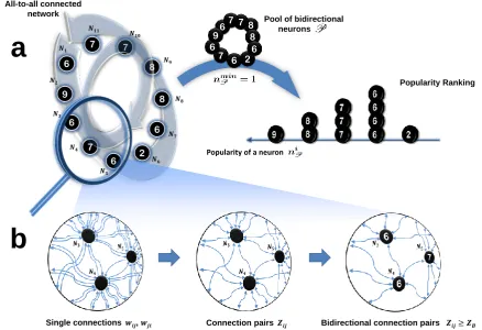
In Fig. 1-3 we show the algorithm implementation on a toy network of N = 11 neurons, all-to-all connected and labelled asN1, N2, . . . N11 (Fig. 1a,left). For simplicity, instead of usingNi when referring

to the neurons of the example, we assume that indices likeivary directly in the setN1, N2, . . . N11. Moreover,

for a better understanding, in Tab. 1 we report a list of the symbols used and their description.

Step 1. Neurons popularity ranking. From the full network’s connectivity W (Fig. 1b, left), we derived the relative strength Zij of each pair of neurons (Fig. 1b, middle), given by equation (2), and we

assess their bidirectionality using the threshold ZB defined in equation (3). This allows assigning to each

neuron i a numberni representing how many bidirectional pairs that neuron forms in the entire network (Fig. 1b,right).

Based on this information, neurons are initially entered in a bidirectional poolPdepending on a minimum required number of bidirectional pairs nmin

P , which can be arbitrarily chosen (Fig. 1a, middle). Neurons

that do not meet thepool entering condition ni_≥nmin

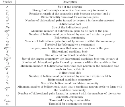
Symbol Description

N Size of the network

wij Strength of the single connection from neuronj to neuroni

Zij Relative strength of the connection pair between neuronsiandj

ZB Bidirectionality threshold for connection pairs

ni Number of bidirectional pairs formed by neuroniin the entire network

P Bidirectional pool

NP Size of the bidirectional pool

nmin

P Minimum number of bidirectional pairs to be part of the pool

ni

P Number of bidirectional pairs formed by neuroniwithin the pool

C Bidirectional community

ni

C Number of bidirectional pairs formed by neuroni within the community

ϑC Threshold for belonging to a community

Cmax

i Largest possible community that neuronican form in the pool

˜

B Bidirectional candidate blob

N_B˜ Size of the bidirectional candidate blob

Nmax_˜

B Size of the largest community the bidirectional candidate blob can be part of

ni

˜

B Number of bidirectional pairs formed by neuroniwithin the candidate blob

nmin

˜ B

Minimum number of bidirectional pairs that each neuron in the candidate blob needs to form within it

B Bidirectional blob

ni

B Number of bidirectional pairs formed by neuroniwithin the blob

˜

C Bidirectional candidate community

N_C˜ Size of the bidirectional candidate community

nmin_˜

C

Minimum number of bidirectional pairs that a candidate neuron needs to form with the candidate community

ni

˜ C

Number of bidirectional pairs formed by neuroniwith the members of the current candidate community

ϑnoise Threshold for noisy communities

ϑω Threshold for communities merger

Table 4.1List of the symbols used for the algorithm description and their meaning.

requirement for being part of a community. As a consequence, the bidirectional pairs that these excluded neurons form in the network also cannot be part of any community, hence they should be subtracted from the

ni _{of the involved neurons. Therefore, after P is formed, neurons are subject to the pool staying}

condition ni

P ≥nminP , whereniP is the number of bidirectional pairs formed only withinP. Nodes violating

this inequality are excluded from P and so are their bidirectional pairs. The pool is therefore reduced and

ni

P need to be updated. This iterative process stops whenniP ≥nminP ∀i ∈ P or when the number of

neurons left in the pool is below the noise threshold (meaning that an eventual community can be considered as a random happening, see below). In the first case, the finalP is the working material for the next steps, whereas in the second case the entire algorithm ends with no communities found.

Differently from the following steps, nodes that are left out ofP are definitely lost, as they will not be reconsidered again. Hence, the value assigned tonmin

P has to be carefully evaluated: limiting the number of

neurons in the pool will greatly reduce the computational cost of the rest of the algorithm; however, the risk of not including neurons that are actually part of a community increases. Throughout this paper we adopt the ”safe” choicenmin_P = 1, for whichP coincides with the whole network whenN andZB are sufficiently

large like the ones we use. This is also the case of the toy network we are considering in this section (all neurons of the network are admitted to the pool, see Fig. 1a).

Neurons in P can be sorted in a popularity ranking based solely on ni_P (Fig. 1a, right). In doing so, nodes with the same value ofni

P are treated as identical because we are (temporarily) losing all the detailed

information of which pairs of neurons are effectively connected with each other. Step 2 below is built only upon the popularity ranking, therefore without the need to access this detailed information. This allows to save a considerable amount of computational resources and to speed up the research, while still obtaining great results in terms of community detection.

Popularity ranking is a preliminary step, deterministic and with no approximations (i.e. there is no loss of information) as long as the thresholdnmin

P is kept to a low value. From now on we will be working only

8 6

8 7

2 6 7

6 9

6

8

6 7

8 7

2 6 7 6

9

6

Popularity of a neuron

7

Pool of bidirectional neurons f

𝑵𝟏

𝑵𝟐

𝑵_𝟑

𝑵_𝟒

𝑵_𝟓

𝑵_𝟔

𝑵𝟕

𝑵𝟖

𝑵_𝟗

𝑵𝟏𝟎

𝑵𝟏𝟏

All-to-all connected network

Single connections 𝒘_𝒊𝒋, 𝒘_𝒋𝒊 Connection pairs 𝒁𝒊𝒋 Bidirectional connection pairs 𝒁𝒊𝒋≥ 𝒁𝑩 Popularity Ranking

a

b

Figure 1 Algorithm Step 1: Neurons popularity ranking. AAll-to-all toy network ofN= 11 neurons labelled

fromN1toN11(left). Each neuroniis associated with an integer representing the number of bidirectional connections made by iin the entire network, ni. Neurons meeting the thresholdnminP = 1 are entered in a bidirectional pool

P (middle), and here they are sorted in a popularity ranking according to the number of bidirectional connections

made within the pool,niP (right). In this example, network and pool coincide. BZoom on a portion of the network highlighting the procedure to obtain

ni _{: The initial directed network{w}

ij, wji}(left) is mapped into an undirected

network of single connection pairs{Zij}(middle). nicounts how many of these pairs fall in the bidirectional domain

(right). This quantity is used as initial criterion to enter the neurons in the poolP(see text).

Step 2. Blob search. Our heuristic approach consists in using the popularity ranking to narrow the research to the regions in P where it is more likely to find a community. The key observation is that once we give a formal definition of community like equation (4), we can use it a basis for a reliable heuristic search. On the left hand side of equation (4) we have the number of bidirectional pairs formed by neuron i within the community C, which, by using the notation introduced in this section, can be rewritten as ni

C. As pointed out earlier, these quantities are unknown; however, they are upper bounded byniP, which

corresponds to the case where all the bidirectional pairs that a neurons forms are part of the same, unique community. We can invert this argument and derive from equation (4) the size of the largest community that each neuron can potentially form within the pool:

|Cmax i |=

ni

P

ϑC

+ 1 ∀i∈ P. (5)

|Cmax

i |does not take into account which are the neurons connected with neuronithrough theniPbidirectional

connections. As a consequence, all the NP =|P|relations of equation (5) are uncoupled, differently from

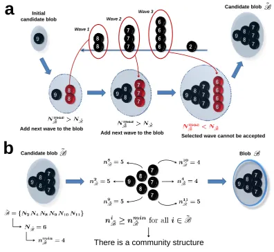
what happens in the community definition. Starting from equation (5), this second step aims at filling the gap with equation (4) by progressively incorporating these element that have been discarded, hence producing as a result sets of neurons in P that satisfy the full community definition. The goal of this step is indeed to find the largest possible communities in the network. This is done through a recursive two-step procedure, depicted in (Fig. 2):

Add next wave to the blob

Candidate blob Initial

candidate blob

Add next wave to the blob

Selected wave cannot be accepted

Wave 1

Wave 2

Wave 3

a

Blob

There is a community structure

b

Figure 2 Algorithm Step 2: Blob search. APart 1: Detecting a candidate blob ˜B. The research starts with

the highest ranked neuron as the only one in ˜B (top left). The other neurons left in the ranking are divided into waves depending onniPand are progressively added to the candidate blob until the conditionNBmax˜ > NB˜is violated

(middle), see explanation in the text. IfNBmax˜ < NB˜, as in this example, then ˜Bis the set of neurons found before

adding the current wave (top right). BPart 2: Candidate blob validation. The full community definition is restored within ˜B, giving the minimum number of bidirectional pairs that each neuron of the blob needs to form within the blob itself,nminB˜ (left). In this example all the neurons in the candidate blob meet this requirement (middle), as they are all-to-all bidirectionally connected except for the pairN4,N10. The candidate blob satisfies then the complete community definition and gets the status of blobB(right).

bidirectional candidate blobB˜. Formally, ˜Bis a set of neurons such that:

ni_P ≥ϑC

|B| −˜ 1 ∀i∈B˜ withB˜as large as possible. (6)

Respect to equation (5), with equation (6) we are restoring the coupling between the equations, that is an essential feature of the community definition. On the other hand, the approximation that we are making respect to equation (4) is clear when we compare the two relations: neurons are included in

˜

Bnot because of the number of bidirectional connections that they form within ˜B, as the community definition would require, but depending on the total number of bidirectional connections that they form in the entire pool,ni_P.

Note that ˜B does not coincide with the potential community that the most popular neuron can form (maxi∈P|Cimax|), but it is highly likely that such a neuron is part of ˜B. In other words, the most

popular neuron i∗ = argmax_i∈P|Cmax

i | is the node that has the highest probability in the entire

network to belong to ˜B, hence it is the first one to be recruited. In the example, i∗ _{= N}

2, with 9

bidirectional pairs formed in the pool (see Fig. 2a,top left). The other neurons are organised in waves, formed by identically ranked nodes, which are evaluated one at a time in a descending order (Fig. 2a,

N_B˜and the sizeN_Bmax˜ of the largest possible community the entire set ˜Bcan be part of, based on the

popularity ranking. Since for each neuron this is given by equation (5), then, for the candidate blob as a whole,Nmax_˜

B is determined by the last wave of neurons included:

N_Bmax˜ = min

i∈_B˜|C

max

i |. (7)

At the beginning, ˜B={i∗}, henceN_B˜= 1 andN_Bmax˜ =|Cimax∗ |. As we progressively recruit waves of

neurons,N_B˜increases whereas N_Bmax˜ decreases. As long asN_B˜< N_Bmax˜ then ˜B can potentially be a

community and we can keep on recruiting the next wave of neurons to investigate whether a larger candidate blob (which could lead to a larger community) is possible. When the inequality is no longer satisfied then the process of recruiting neurons stops. We can have two scenarios: N_B˜> N_Bmax˜ means

that some neurons in ˜B, the most recently added ones, do not have enough bidirectional pairs: even in the most optimistic case where all these pairs are within ˜B, these neurons do not meet the community threshold, given the actual size of ˜B. Thus, the largest possible candidate blob is the one found at the previous iteration. This is the case of the toy network we are considering, as shown in Fig. 2a,top right. The second scenario is whenN_B˜=N_Bmax˜ , and the largest possible candidate blob is the set of

neurons found at the current iteration.

• Part 2. At this stage we have a set of neurons, a candidate blob ˜B (Fig. 2b, left), that satisfies equation (6): according to the number of bidirectional connections that each of them forms in the pool, ˜B is suitable to form a community. We can therefore move on and restore the full community definition, equation (4), by computing the number of bidirectional connectionsni_˜

Bthat each neuron in

˜

Bforms within ˜Bitself (Fig. 2b,middle). In other words, we are substitutingni

P withni_B˜in equation

(6), obtaining exactly the community definition. Thus, if each neuron in ˜Bsatisfies the condition, then there is a community structure and we call it abidirectional blob B(Fig. 2b,right): a set of neurons that certainly contains at least one bidirectional community.

If the community definition is not satisfied, then we withdraw those neurons that violate it to obtain a new ˜Band to applyPart 2 again. This refinement process continues until the algorithm finds a blob Bor until ˜B contains only one neuron, meaning that there is no blob.

Whenever this step gives a non empty blob as a result, then we proceed withStep 3 below to finally find the communities that are present inB. After this, we temporarily eliminate from the pool all the neurons that have been detected as being part of a community so far, and to this modified pool we apply Step 2

from the beginning. Therefore, if a neuron is found to be part of a community, it does not get the chance to be evaluated again for being included in other blobs, meaning that blobs are all disjointed sets. This is one of the reasons why we introduceStep 3 below, which is built to detect overlapping communities.

The procedure continues until there is no blob found. In this case the entire algorithm goes to an end and its final outcome are all the bidirectional communities found so far within the previously detected blobs. Thus, the result of this step is a set of non-overlapping blobs, each of them containing for sure at least one bidirectional community.

Step 3. Looking into a blob: the friendship algorithm. The setBthat we obtain at the end ofStep 2 certainly forms a community, as it satisfies the definition. However: i) two different communities, or at least parts of them, may be detected within the same blob (resolution problem). ii) The method does not correctly identify overlapping communities. If there is an overlap between any of them, the above procedure assigns the intersection region to only one community (overlapping problem). iii)Mistakes may occur during the identification process: some neurons that are originally part of a community may have been left out of the blob that contains that community, we call themgood friends, whereas some other neurons may have been erroneously included inB, we call themfalse friends (accuracy problem).

In order to address these issues, at this stage we define a procedure that builds up a community neuron by neuron through direct verification of the definition. This approach is much more feasible and robust at this stage rather than at the very beginning, for two reasons: i)we apply it to a very limited set of neurons, i.e. the blobB, andii) we already know that these neurons are relevant in terms of community structure.

7

7

7 7

Blob

Community core

7 7 7

Initial candidate community

Current random candidate

Candidate accepted

Nodes left in the blob Final candidate community

a

b

The 3 highest ranked neurons

that are all to all connected

through a bidirectional pair

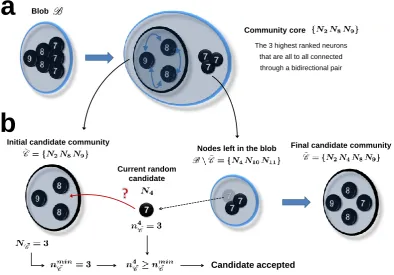
Figure 3 Algorithm Step 3: Friendship algorithm. ADetecting the candidate community core: The highest

ranked neurons in the blob that are also all-to-all bidirectionally connected. B Building a candidate community: Starting from the core (left), one of the neurons that are left in the blob is randomly selected at a time and, based on the community definition, its inclusion in the candidate community is evaluated (middle). Here we show only the first iteration with the neuronN4: Because it forms a bidirectional connection with all the 3 neurons in ˜C(n4C˜= 3), it can be accepted, resulting in a bigger candidate community for the next iteration (right).

nodes maximise the probability of having three neurons being part of the same community, since they are the highest in the ranking. On the other side, the choice of having a core of only two neurons does not seem very reliable because, due to the random generation process of connections in the network (see below), the event that two neurons are connected with a bidirectional pair is very common, even among neurons that are not part of any community. Once we identify the candidate community core, in each iteration we randomly select a neuron in the blob and we ask if it satisfies the community definition (Fig. 3b): given the current size of the candidate communityN_C˜, by using the definition equation (4) and rounding up the

result, we have the minimum number of bidirectional connectionsnmin

˜

C that thecandidate neuron needs to

form with the current members of ˜Cin order to join it.

In Fig. 3b we show the procedure for the first iteration only, where ˜C ={N2N8N9}, hence N_C˜ = 3,

nmin

˜

C = 3, andN4is the randomly selected node. This neuron forms 7 bidirectional connections in the entire

network, but at this stage this is not relevant anymore. What matters is that it forms a bidirectional pair with each of the neurons in the current candidate community (n4

˜

C = 3), meaning that it is ”friend” with all

of them and thus it can clearly be accepted in ˜C. In the next iteration, the candidate community is then ˜

C ={N2N4N8N9}, which results inN_C˜= 4 and nmin_C˜ = 3 again. Thus, the neuron that will be selected,

either N10 or N11, needs to form at least 3 bidirectional connections with the 4 candidate community’s

members in order to join it. This is exactly what happens in this example, and, since in the last iteration also the last neuron turns out to have enough friends in ˜C(for which it will beN_C˜= 5 andnmin_˜

C = 4), the

final candidate community will coincide with the blob: ˜C={N2N4N8N9N10N11}.

Most likely, the above procedure returns a set that is a single, well consistent candidate community, hence solving the resolution problem. However, it might not be the original complete community: good friends may be left out, most likely in the blob B but also in the pool P. Therefore, we start recruiting for a second time with the condition of satisfying the community definition, first among the neurons left in the blob and then within the pool (good friends inclusion). This procedure, together with the false friends expulsion, addresses the accuracy problem. Moreover, recruitment among neurons in the pool allows to consider for the current candidate community also neurons that have been previously included in other blobs or communities, hence solving the overlapping problem. In our example, there are no neurons left in the blob so we check the ones in the pool: N1, N3 and N7 are recruited whereas N5 and N6 are left out,

giving finally a community candidate of 9 neurons that coincides with the original true community.

Step 4. Candidate community global control. As pointed out earlier, based on Esposito et al. (2014) [Esposito et al., 2014], for a set of neurons to be a bidirectional communityC, its symmetry measure equation (1) must exceed a threshold valuesB, which depends on the distribution of connections considered.

Now that we isolated a candidate community from the rest of the network, we are in the position of applying this criterion. Candidate communities that do not pass this test are sets that cannot be qualified as commu-nities. Note, however, that they are still bidirectional communities in the sense of our topological definition equation (4). Since this definition is threshold-based, it introduces a binary criterion with subsequent loss of information. The definition is guidance for community detection that reduces the weighted network to an un-weighted one. Thus, once the research has been successful, the complete information stored in the weights needs to be recovered and the actual identity as bidirectional community can be finally evaluated by means of the symmetry measure.

Sets that cannot be qualified as communities present an excess of bidirectional pairs due to the random generating process, which made these sets to be detected as possible communities, but failure in the sym-metry measure test means that the rest of the pairs are far from being bidirectional, hence pulling the value of the symmetry measure down within the randomness boundaries. This is no evidence that learning took place in the specific set as a whole. Statistically, this situation is likely to happen for small sets of neurons, and indeed this is when we observe failure of the symmetry measure test. These sets of neurons are therefore safely withdrawn.

Step 5. Noisy candidate communities identification. Besides the real communities that are present in the network as a result of learning, communities can be also formed out of chance, due to the randomness in the network’s connectivity: it is highly likely that small sets of 4−5 neurons show community properties and thus will be detected as such. Since the probability of randomly forming a community dramatically drops with the size, we can define a noise threshold ϑnoise and discard all sets below such a threshold.

This clearly fixes a lower limit to the resolution of the algorithm. However, the maximum size of a random community, which ideally corresponds to such a threshold, grows with the size of the network in a way that is sub-linear, allowing to set a unique, relatively small threshold for all the networks with a large size that does not affect the overall performance.

Step 6. Single community reduction. At this stage we have single communities C, but we might have a finalredundancy problem, especially for networks of small size: it can happen that the same original community has been detected more than once, every time with different false friends included and good friends left out. It can also happen that the original community is broken into two overlapping parts detected as different communities. The final step is therefore trying to resolve these issues calculating the overlap degrees between each pair of communities. Pairs with an overlap exceeding the overlap threshold

ϑω are merged together and the symmetry measure is used as an evaluating criterion: if the value on

the merged community is higher than the values of the single communities, then the merged community definitely replaces the two single ones, otherwise they are kept separate.

Network and communities generation: benchmark procedure

To test the above algorithm, we generatedin silico data representing several different scenarios, which will be discussed in the Results section alongside the algorithm performance. Below, we describe the general procedure used to produce a connectivity matrix for a network containing bidirectional communities.

The first step for creating a bidirectional community is to decide the value of its symmetry measure, which has to be in the range [sB,1] [Esposito et al., 2014]. By definition, this gives the mean value of the

the pairs form a Gaussian distribution. Therefore, for each community in the network, we generated the set of {Zij} according to a Gaussian distribution with mean hZi and standard deviation σ, which is a

free parameter. We recall that Z is a variable ranging from 0 to 1 and that the bidirectionality region is [0, ZB]. Based on this, two issues may arise when we generate the pairs, related to the two boundaries and

to the choice ofσ: i) some of theZij could be negative. If this is the case, the tails of the distribution are

symmetrically folded towards the inside so as to guarantee the non-negativity of the{Zij} and to preserve

the mean value of the distribution. ii) A considerable part of the distribution could fall in the randomness domain (Z > ZB), meaning that many pairs will not be classified as bidirectional. As a consequence, some

neurons may not form the minimum number of bidirectional pairs required by the community definition, resulting in the whole set not being a community anymore. To avoid this issue, we make sure that the integral of the Gaussian in the bidirectional region, which gives the probability of forming a bidirectional pair℘B, exceeds the community thresholdϑC.

Once we have the set of{Zij} for each community, we can generate the single connectionswij. A first

half of them is directly drawn from the uniform distribution in [0,1], be the upper (or the lower) triangular part of the community’s connectivity matrix. This first half, together with the{Zij}, is used to compute the

second half of the single connections by means of equation (2). The rest of the connections in the network are drawn from the uniform distribution in [0,1].

Overlaps between communities are governed by the set of parameters{ωλρ}representing the fraction of

the community ρthat is in common with the communityλ:

ωλρ=

|Cλ∩ Cρ|

|Cρ|

(8)

We allow overlaps only between subsequent pairs of communities. In other words, we can progressively enumerate the communities in the network in such a way each of them overlaps at most with only the previous and following one. Formally: ωλρ = 0 if|λ−ρ| ≥2, leading to a tridiagonal matrix of overlaps.

In cases of overlap between two communities, after having generated the first community, the mean of the pairs in the intersection is computed and it is used to offset the mean of the Gaussian distribution for the rest of the pairs in the second community, so as to preserve the value of the symmetry measure that we chose.

The set of parameters{sλ}, {σλ}, {ωλρ} we introduced here for the connections generation, together

with the size of communities {Nλ} and network N, entirely define the structure of a network, but they

do not uniquely determine its connectivity because all the connections are generated through the above mentioned random process. Due to the presence of random elements in both data generation and detection procedure, for each combination of parameters we consider, we repeat the experiment niter = 100 times.

Each experiment, or run, consists in generating the network connectivity as described above and applying our detection algorithm. Cumulative and averaged results are displayed in the appropriate section.

Analysis of the results: measuring successful detection

At the end of each run, on one side we have the communities that we generated at the beginning, i.e. the real communities, and on the other side those detected by the algorithm. One way of measuring the quality of the results is to count how many good neurons have been detected. However, since this is going to be displayed as an average over the runs, we may lose too much information about the single run. Also, as pointed out earlier, failure in detecting single neurons may still happen despite the bulk of the community has been correctly identified.

Therefore, we introduce a criterion to determine successful community detection: whenever the number of neurons in a detected community equals at least a fraction ϑrecog of the neurons in a real community,

we count that real community as successfully identified. If there is more than one detected community for which this happens relatively to the same real community, then the one with the highest percentage is considered to be one matching the real community and the others are counted as false communities, unless they result to match some other real community in the network. We chooseϑrecog= 75% as in our opinion

Thresholds

The algorithm described above makes use of 5 customisable thresholds, see Tab. 1. Throughout this paper we keep them fixed at their respective values. Since we assume a uniform distribution of connections prior learning, we can directly rely on the results of Esposito et al. 2014 [Esposito et al., 2014] for uniform distributions: by fixing a level of confidence atp= 0.05, the bidirectionality threshold we use issB= 0.6954,

which in turn givesZB = 0.3046. The thresholdϑCfor community existence is rather arbitrary and it can be

fixed according to how dense we require the communities to be. In the present study we choose ϑC = 75%.

Concerning the noise effect, after observing the size of the noisy communities detected by the algorithm, we fix ϑnoise = 30. For the other thresholds, also arbitrary, we use nmin_P = 1 as a safe choice (as previously

stated) and ϑω= 25% as a limit case before two communities can be considered as part of a single bigger

one (after evaluation of symmetry measure, seeStep 6).

Results

In this section we present the results obtained by applying the community detection algorithm to networks of neurons with different community structures. In all the cases, we assume that the given network is the final product of a learning process that shaped the connections of some sub-regions away from the initial uniform distribution, to form what we called bidirectional communities, equation (4). The rest of the connections remain unchanged and therefore they are uniformly distributed. Network connectivity is generated according to the procedure outlined in Methods section.

Since the learning process is not explicitly simulated here, we have total control on the final structure of the network, through the tuning of 6 sets of parameters: the size of the networkN, the number of commu-nitiesν, the size of communities{Nλ}and the overlap between communities{ωλρ} define the architecture

of a network. The symmetry measure of the communities{sλ}and the standard deviation of the connection

pairs in the communities{σλ}define how much a community has been shaped towards bidirectionality.

The way the algorithm is constructed, we expect that strong bidirectional communities, i.e. withs→1 and small σ, are the easiest to detect, compared with bidirectional communities with s → sB and large

standard deviation. The degree of difficulty in the detection of a community can be derived from the way we generate the community itself. Indeed, as pointed out in the Methods section, s and σdetermine the number of bidirectional pairs that each neuron forms in the community, through a random process. Thus, necessary condition for a set of neurons to be a community (and therefore to be detected) is that this number exceeds the threshold for community existence. Also, the closer this number to the threshold (from above), the more difficult the detection of the community.

Each simulation consists ofniter= 100 runs, each of them starts with communities and network

genera-tion, continues with the communities’ detection algorithm and finally ends with the evaluation of the results, where we compare detected and generated communities. To evaluate the algorithm performance, we use two indicators for each community generated in the network. The first quantity counts how many times a community has been successfully detected during theniteriterations (see Methods). Once a community has

been correctly identified, the second indicator measures how many nodes of the generated community have been detected, and displays this information as an average percentage across niter iterations and relative

to the total number of nodes in the generated community. Additional indicators for the number of false communities detected and for the percentage of false neurons in a correctly detected community complete the evaluation.

Networks with a single community

Alongside the size of the community, we introduce the community to network ratiorc/n=NC/N, which

is a more significant indicator to assess the algorithm performance. A complete evaluation (at least in the single community case) requires, therefore, carrying out 3 different analyses, corresponding to fixing one of the three quantitiesNC, N, rc/nwhile varying the other two.

Single, size-varying community in a network of fixed size

We begin the analysis of the algorithm performance with the most common and typical problem: given a network, we want to know if there is a community and of which size. Therefore, we fix the size of the network at N = 5000 neurons and we systematically vary the size of the community in the set {75,100,250,500,750,1000,2500}. The community is generated with sC = 0.75 and σC = 0.05,

result-ing in a probability of formresult-ing a bidirectional pair ℘B = 0.863. Correctly, ℘B > ϑC (see Network and

Time per neuron [s] 0 0.02 0.04 0.06 0.08 0.1

200 400 800 2000 4000 8000

Network size 0.025 0.05 0.1 0.25 0.5 1

Ratio Community to Network

Time per neuron [s] 0 0.02 0.04 0.06 0.08 0.1

0.015 0.02 0.05 0.1 0.15 0.2 0.5

Ratio Community to Network

75 100 250 500 7501000 2500

Community size

Community Detection 0

20 40 60 80 100

50 75 100 150 250 350 500 750

Community size

Neurons Detection % 0 20 40 60 80 100

200 400 800 2000 4000 8000

Network size

Community Detection 0

20 40 60 80 100

200 400 800 2000 4000 8000

Network size

Neurons Detection % 0

20 40 60 80 100

0.015 0.02 0.05 0.1 0.15 0.2 0.5

Ratio Community to Network

Community Detection 0

20 40 60 80 100

0.015 0.02 0.05 0.1 0.15 0.2 0.5

Ratio Community to Network

a

b

c

e

f

d

g

h

i

Neurons Detection % 0 20 40 60 80 100

50 75 100 150 250 350 500 750

Community size

Time per neuron [s]

0.2 0.4 0.6

50 75 100 150 250 350 500 750

Community size

1000 1500 2000 3000 5000 70001000015000

Network size

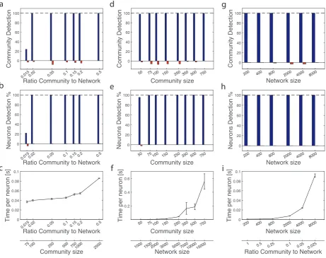
Figure 4 Algorithm Performance for the case of single community of sC = 0.75 and σC = 0.05

embedded in a network. A - C Network’ size fixed at N = 5000 neurons while varying community’ size.

D - FRatio community to network fixed at rc/n= 0.05 while varying both network’ and community’ size. G - I

Community’ size fixed at NC = 200 neurons while varying network’ size. All results in each panel are relative to niter = 100 repetitions. A, D, G Cumulative community detection. Blue bars: Successful detection, Red upside

down bars: False detection. The dashed line represents the best possible performance of correctly detecting the

community all the time. B, E, H Average percentage of neurons detection, relative to the size of the generated community. Blue bars: Good neurons,Red upside down bars: False neurons. C, F, ISimulation time per neuron in the network. Error bars represent standard error. Note that the scale of all x-axes is logarithmic.

In Fig. 4a we report the results concerning community detection: blue bars show the cumulative number of successful detection of the generated community, whereas the upside down red bars count the number of false communities. Similarly, Fig. 4b shows the average percentage of good neurons (blue bars) and false neurons (upside down red bars) in the detected community. Blue bars carry what we can call a positive information as we want to maximise them, whereas red bars is what we want to minimise to zero, hence they carry anegative information. The horizontal black dashed line marks the optimality level for positive information: when for the same value ofrc/n both bars of Fig. 4a,b hit this level means that the algorithm

has detected all the neurons forming that community all the time. For the values considered here, this is almost always the case, except for the smallest community case where detection of the community is successful only 20% of the times. Note that whenever this community is identified, the algorithm correctly recruits all the good neurons (the blue leftmost bars of 4a,b have the same height). As expected, these results suggest that the bigger the size of the community the easier to detect it, with a critical value of ∼100 neurons.

the community (by increasing the value of its symmetry measure), the algorithm time is the same (result not shown here). This means that detection time is not affected by the internal structure of the community but only by its size.

Single, size-varying community in a size-varying network with fixed ratio

The above scenario gives only partial information on the goodness of the algorithm, as the size of the network is fixed to a single value: Fig. 4a-c show results when we vary only the size of the community to account for different ratios community to network. However, the task of finding a community of 100 neurons in a network of 1000 nodes might be different from searching for a community of 1000 in a network of 10000 nodes.

Therefore, we investigate a second scenario: a single, size-varying community within a network whose size also varies, in such a way to keep the ratio community to network fixed. We choose a relatively small value rc/n= 0.05, while the size of the community varies between the values{50,75,100,150,250,350,500,750}.

The size of the network varies accordingly from 1000 to 15000. As above,sC = 0.75 andσC = 0.05.

Results are shown in Fig. 4d-f, with the same meaning of quantities and colours as in Fig. 4a-c. Detection is perfect almost all the time, with very few mistakes mostly in the sense of detecting false communities. At first, the performance is fairly independent of the absolute sizes, as expected. A more careful inspection shows that slightly better performances are obtained for larger sizes. The reason could be that for larger networks the fluctuations on the bidirectional pairs formed out of chance become smaller and for the neurons being part of the generated community is easier to stand out of the crowd of nodes, hence the precision of the algorithm increases.

Single, fixed size community in a size-varying network

Finally, to complete the analysis of the single community case, we study the algorithm performance when we increase the size of the network while keeping fixed the number of nodes in the community. We choose a small community of NC = 200 neurons and we vary the size of the network in the set

{200,400,800,2000,4000,8000}. The ratio community to network varies accordingly from 1 to 0.025. Again, sC = 0.75 andσC = 0.05.

Results are shown in 4g-i. Once again, the performance of the algorithm is excellent in the range of values considered, in terms of both positive and negative information. In particular, 4h shows that the algorithm finds exactly the 200 neurons forming the community all the time, with no false neurons. As expected, increasing the size of the network also increases the time needed for the detection, with dependence from the time per neuron of the network that looks quadratic.

Community NC sC σC ωCC0 ℘_B

1 200 0.75 0.05 - 0.86

2 200 0.75 0.05 0.2 0.86 3 500 0.74 0.05 0.1 0.81 4 150 0.74 0.05 0.2 0.81

5 150 0.79 0.1 0 0.81

Table 4.2List of parameter’s values used to generate the community structure in the case of ν= 5 communities.

Column 1: Community progressive number. Column 2: Size of the community. Column 3: Symmetry measure.

Column 4: Standard deviation of the connection pairsZ. Column 5: Overlap with the previous community, expressed

as number of common neurons divided by the number of total neurons in the community. Column 6: Probability that a neuron of the community forms a bidirectional pair, as a result of a Gaussian distribution with parameters based on Columns 3 and 4.

A multiple communities case

0 50 100 Community 4 7500 5000 2143 1500 Network Size 0.100 0.070 0.050 0.030 0.020

Comm 4 Ratio

Comm Detection 3000 Good Neurons False Neurons 0 50 100 Community 3 7500 5000 2143 1500 Network Size 0.333 0.233 0.167 0.010 0.067

Comm 3 Ratio

Comm Detection 3000 Good Neurons False Neurons 0 50 100 Community 2 7500 5000 2143 1500 Network Size 0.133 0.093 0.067 0.040 0.027

Comm 2 Ratio 3000

Comm Detection Good Neurons False Neurons 0 50 100 Community 1 7500 5000 2143 1500 Network Size 0.133 0.093 0.067 0.040 0.027

Comm 1 Ratio

Comm Detection 3000

Good Neurons False Neurons

Time per neuron [s]

0.1 0.2 0.3 0.4

1500 2143 3000 5000 7500

Network size 0.02 0.03 0.05 0.07 0.1

Ratio Community to Network

Av. Community Detection0

1 2 3 4 5 6

1500 2143 3000 5000 7500

Network size 0 50 100 Community 5 7500 5000 2143 1500 Network Size 0.100 0.070 0.050 0.030 0.020

Comm 5 Ratio

Comm Detection 3000 Good Neurons False Neurons

a

f

b

g

c

d

e

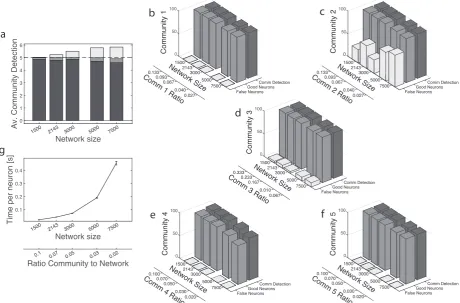
Figure 5 Algorithm Performance for a network with complex structure. Five communities with different

sets of parameters, see Tab. 2, are embedded in the network. Communities’ size are kept fixed while varying network’ size. All results in each panel are relative toniter = 100 repetitions. A Global performance. Dark grey

bars: Successful detection with all communities resolved, grey bars: Successful detection with two communities

unresolved (see text for details), light grey bars: False communities. The dashed line represents the best possible performance of correctly detecting all the five communities all the time. B - FSingle community detection statistics.

Dark grey bars: Cumulative community detection over the 100 repetitions,grey bars: Good neurons,light grey bars:

False neurons. Note that the (expected) discrete amount of false neurons detected in communities 2 and 3 is due to the unresolved cases between these two communities (see text for a discussion). GSimulation time per neuron in the network. Error bars represent standard error. Note that the scale of all x-axes is logarithmic. The ratio community to network below panel g is relative to the smallest community in the network.

Fig. 5a shows the global performance of the algorithm, in the form of stacked bars for each value of the network’s size considered. The dark grey part at the bottom of the bars counts how many times the 5 communities have been correctly detected as 5 different communities, as an average over niter= 100 runs.

The central part in grey shows the average number of times that a community has been detected as an unresolved community, i.e. two overlapping communities detected as a single big one (never more than two). The upper part in light grey shows the average number of false communities. Clearly, as the size of network increases, the number of false communities also increases, but the performance on the 5 true communities remains stable and optimal. Indeed, all the communities are detected almost all the time, either resolved (more than 95% of the time) or unresolved. From a more detailed analysis of the results, it can be seen that when there is an unresolved community this is always the union of the communities 2 and 3 in Tab. 2. This is reasonable as C3 is by far the largest in the network and the overlap of 0.1 with

communityC2 means that they have 50 neurons in common. From the perspective of community 2 this is

a considerable overlap of 25%, which indeed equals the value we chose for the overlap thresholdϑω. It is

therefore a matter of few neurons whether these two communities are merged or not during the last step of the algorithm (see Methods).

unresolved cases between these two communities. In this sense they are not completely false neurons. Finally, community 4 is the only one showing a decrease in the performance as the size of the network increases, with percentages still above 85% for N = 7500. The reason is that C4 is the most difficult to

detect because is the one with the lowest values ofNC, sC andσC.

The last panel, Fig. 5g shows the simulation time per neuron in the network. Note that, compared to the case of a single community, the time needed is nearly five times larger, suggesting that it grows linearly with the number of communities.

Discussion

In this paper we address the problem of structure detection in networks of neurons, which is of crucial importance in the study of connectome in Neuroscience, framing it within the well-known, in Network Theory, community detection problems. By nature, networks of neurons are weighted and directed graphs, which makes the problem of structures searching in these networks one of the most difficult ones to approach. In the general, for most of the problems related to structures detection in Graph and Networks Theory it is not possible to give an exact solution, hence heuristic algorithms are often adopted.

Here we present an algorithm for the detection of a particular class of communities in large scale simulated networks. Thus, this is intended mainly as a tool to help in silico research aiming at understanding the connectome. In the future, the opportunity of having direct access to synaptic weights, and therefore to connectivity matrices, may also allow a direct application of the algorithm to experimental data. Moreover, the algorithm could be of more general interest for pure studies in Networks and Graph Theory and it can be adapted to similar problems in other disciplines where nodes are not neurons.

Differently from cliques, that are very well defined objects, the concept of community is vague and we cannot find a unique definition in the literature. Traditional methods for community searching are either based on cliques or define a community a posteriori, i.e. as the outcome given by the algorithm. Here we propose a different approach by giving a formal definition for communities a priori. We show how having such a definition is an advantage as the algorithm can use it directly for a more efficient and direct research. Also, the method is based on a definition of symmetry measure, which allows manipulating the original connectivity and deal with quantities carrying much reduced information. This implies a loss of information, but we show that results are excellent and there is a great benefit in terms of time and computational resources.

The algorithm we present is based on statistics and it requires that the distribution of the connections is known and is somehow regular: we assumed a uniform distribution, but in principle the method works for any kind of distribution for which it makes sense to define mean and variance. As such, differently from traditional approaches, our method works better for large number of neurons: we show that increasing both the size of the network and the community gives better results. Also, we chose to focus on bidirectional communities, but the procedure can be extended to other kind of communities, for instance unidirectional ones. Indeed, similarly to bidirectional structures, experimental results show also an excess of unidirectional connections in some parts of the brain [Wang et al., 2006,Lefort et al., 2009,Pignatelli, 2009]. Generalisation to sparse networks should be also possible.

The results we present here are relative to worst case scenarios, because the communities are generated with symmetry measure very close to the random domain. For communities that are more markedly bidi-rectional the performance would be even better. Besides measuring the success on community detection, the performance of the algorithm is also evaluated on the false detections: false communities and false neurons within good communities. Based on initial results, to minimise false communities we naively fixed a threshold for a minimum community size at 30 neurons, considering everything smaller as an outcome of the random process used to generate the connections in the network. This limits the resolution of the algorithm: if there are real communities whose size is smaller than the threshold, they will not be detected. Since the average size of communities formed out of random depends on the size of the network, this part of the algorithm can be improved by using a threshold that is a function ofN. Such a function can be de-rived by carrying out a systematic analysis on completely random networks, both theoretically and through simulations.

On the other hand, it is worth noting there is nothing that makes a false community different from a true community, except for the fact that the latter has gone through a learning process. A possible approach to solve this problem could be therefore to track the evolution of the connectivity whenever possible. After having detected the communities, looking back at the history of their connections could give important insights about which sets really experienced a learning process.

only highly significant bidirectional communities, if any. We can tune the thresholds as we like for a stricter search, which would require also less computational time. Once we have the outcome, we can then gradually relax the values of the thresholds for a broader search, if we need.

The full algorithm is the combination of two algorithms executed one after the other. The first sub-algorithm alone already gives excellent results, especially for single community detection, with a massive reduction of the running time. Indeed, the second sub-algorithm is essential for dealing with overlaps and for resolving two communities that have been detected as a big one. Also, due to the statistical approach of the algorithm, it is possible to evaluate the level of noise (bidirectional pairs formed out of chance) and take it into account from the beginning of the procedure. This would allow to withdraw a consistent fraction of neurons before executing the two sub-algorithms and therefore to greatly reduce the number of neurons for the search. These aspects need to be further investigated, together with the possibility of introducing parallel computing, to improve on the computational time requirements.

References

[Albert and Barab´asi, 2002] Albert, R. and Barab´asi, A.-L. (2002). Statistical mechanics of complex net-works. Reviews of Modern Physics, 74.

[Ball et al., 2011] Ball, B., Karrer, B., and Newman, M. E. J. (2011). Efficient and principled method for detecting communities in networks. Phys Rev E Stat Nonlin Soft Matter Phys, 84(3 Pt 2):036103.

[Barab´asi and Oltvai, 2004] Barab´asi, A.-L. and Oltvai, Z. N. (2004). Network biology: understanding the cell’s functional organization. Nat Rev Genet, 5(2):101–113.

[Bassett and Bullmore, 2009] Bassett, D. S. and Bullmore, E. T. (2009). Human brain networks in health and disease. Curr Opin Neurol, 22(4):340–347.

[Bomze et al., 1999] Bomze, I. M., Budinich, M., Pardalos, P., and Pelillo, M. (1999). Handbook of Combi-natorial Optimization. Kluwer Academic Publishers, Norwell, USA.

[Bondy and Murty, 2008] Bondy, A. and Murty, U. (2008). Graph Theory. Springer.

[Brandes et al., 2006] Brandes, U., Delling, D., Gaertler, M., Grke, R., Hoefer, M., Nikolski, Z., and Wagner, D. (2006).On Modularity - NP-completeness and Beyond. Universit¨at Karlsruhe, Fakult¨at f¨ur Informatik, Bibliothek.

[Bressler and Menon, 2010] Bressler, S. L. and Menon, V. (2010). Large-scale brain networks in cognition: emerging methods and principles. Trends Cogn Sci, 14(6):277–290.

[Bullmore and Sporns, 2009] Bullmore, E. and Sporns, O. (2009). Complex brain networks: graph theoret-ical analysis of structural and functional systems. Nat Rev Neurosci, 10(3):186–198.

[Clopath et al., 2010] Clopath, C., Buesing, L., Vasilaki, E., and Gerstner, W. (2010). Connectivity reflects coding: A model of voltage-based stdp with homeostasis. Nat Neurosci, 13:344–52.

[Cook, 1971] Cook, S. A. (1971). The complexity of theorem-proving procedures. In Proceedings of the Third Annual ACM Symposium on Theory of Computing, STOC ’71, pages 151–158, New York, NY, USA. ACM.

[Danon et al., 2005] Danon, L., Duch, J., Diaz-Guilera, A., and Arenas, A. (2005). Comparing community structure identification. J. Stat. Mech.

[Diestel, 2010] Diestel, R. (2010). Graph Theory. Springer-Verlag Berlin Heidelberg.

[Esposito et al., 2014] Esposito, U., Giugliano, M., van Rossum, M., and Vasilaki, E. (2014). Measuring symmetry, asymmetry and randomness in neural network connectivity. PLoS One, 9(7):e100805.

[Esposito et al., 2015] Esposito, U., Giugliano, M., and Vasilaki, E. (2015). Adaptation of short-term plastic-ity parameters via error-driven learning may explain the correlation between activplastic-ity-dependent synaptic properties, connectivity motifs and target specificity. Front Comput Neurosci, 8:175.

[Fortunato, 2010] Fortunato, S. (2010). Community detection in graphs. Physics Reports, 486(3-5):75–174.