This is a repository copy of An efficient screening method for computer experiments. White Rose Research Online URL for this paper:
http://eprints.whiterose.ac.uk/84123/ Version: Accepted Version
Article:
Boukouvalas, A, Gosling, JP and Maruri-Aguilar, H (2014) An efficient screening method for computer experiments. Technometrics, 56 (4). 422 - 431. ISSN 0040-1706
https://doi.org/10.1080/00401706.2013.866599
Reuse
Unless indicated otherwise, fulltext items are protected by copyright with all rights reserved. The copyright exception in section 29 of the Copyright, Designs and Patents Act 1988 allows the making of a single copy solely for the purpose of non-commercial research or private study within the limits of fair dealing. The publisher or other rights-holder may allow further reproduction and re-use of this version - refer to the White Rose Research Online record for this item. Where records identify the publisher as the copyright holder, users can verify any specific terms of use on the publisher’s website.
Takedown
If you consider content in White Rose Research Online to be in breach of UK law, please notify us by
An efficient screening method for computer
1
experiments
2
Alexis Boukouvalas
Aston University, United Kingdom
and
John Paul Gosling
University of Leeds, United Kingdom
and
Hugo Maruri-Aguilar
Queen Mary, University of London, United Kingdom
3
October 30, 2013
4
Abstract
5
Computer simulators of real world processes are often computationally expensive
6
and require many inputs. The problem of the computational expense can be handled
7
using emulation technology; however, highly-multidimensional input spaces may
re-8
quire more simulator runs to train and validate the emulator. We aim to reduce the
9
dimensionality of the problem by screening the simulator’s inputs for non-linear effects
10
on the output rather than distinguishing between negligible and active effects. Our
11
proposed method is built upon the elementary effects method for screening (Morris,
12
1991) and utilises a threshold value to separate the inputs with linear and non-linear
13
effects. The technique is simple to implement and acts in a sequential way in order to
14
keep the number of simulator runs down to a minimum, whilst identifying the inputs
15
that have non-linear effects. The algorithm is applied on a set of simulated examples
16
and a rabies disease simulator where we observe run savings ranging between 28% and
17
63% compared to the batch elementary effects method. Supplementary materials for
18
this paper are available online.
19
Keywords: Morris design, Sensitivity analysis, Variable selection.
20
technometrics tex template (do not remove)
1
Analysis of complex computer simulators
22
Formal design and analysis of computer experiments stems from the seminal paper by Sacks
23
et al. (1989). In recent years, computer experiments have been used to make climate
pro-24
jections (Hargreaves et al., 2004), investigate biological processes (Wedge et al., 2009) and
25
estimate national carbon balances (Kennedy et al., 2008). In many applications,
emula-26
tors are constructed as efficient surrogate alternatives to expensive computer simulators
27
(O’Hagan, 2006). Further analyses are then carried out on the emulator; for example,
sen-28
sitivity analyses or prediction of response at new points. However, even when using the
29
emulator technology, the analysis of complex simulators can be restricted by the number
30
of input dimensions. In the present paper, we introduce a sequential screening procedure
31
to identify inputs that have a non-linear effect on the output. Our proposal stems from
32
the elementary effects (EE) method introduced in Morris (1991), and consists of sequential
33
estimation coupled with a space-filling criterion. Estimation of model behaviour is a
com-34
mon practice in sensitivity analysis (Morris, 1991) and use of space filling design ensures
35
reasonable coverage of the input space (Campolongo and Braddock, 1999). There exist a
36
wide range of methods in the literature to estimate functional effects. Screening methods
37
allow for efficient estimation of effects using a minimal number of simulator evaluations.
38
Variance-based sensitivity analyses methods (Saltelli et al., 2000) offer more precise results
39
in terms of the percentage of variance explained by each input factor and their interactions.
40
However, these methods require many more model runs and are employed at a later stage
41
of simulator analysis than screening algorithms.
42
Our aim in this paper is to develop a method that identifies inputs with non-linear
43
effects on the output. Morris (1991) considers screening for factors with linear, non-linear
44
or interacting effects, defined as active. Identification of inputs with active effects is the
45
usual aim of screening, also known as variable selection. Our focus is to distinguish factors
46
with non-linear or interaction effects from factors with linear or negligible effects. It is of
47
interest to identify the latter since they can be dealt with more simply in subsequent stages
48
of simulator analyses as discussed in Section 4. Screening methods are further discussed in
49
Section 2. We review the EE method in Section 3 and introduce our sequential method and
50
its properties in Section 4. We compare the method to other popular screening methods
through a simulated example in Section 5 and finish by demonstrating our method on a
52
computer model of rabies disease spread in Section 6.
53
2
Screening approaches
54
In classical experimentation on physical processes, screening usually incorporates some of
55
factorial designs, fractional factorial designs, nonregular orthogonal arrays, or optimal
de-56
signs. However, without further model assumptions, sequential use of such designs is not
57
straightforward and cannot be utilised to identify a nonlinear effect. When the number of
58
inputs dimensions is very large, but it is expected a priori that only a small subset of them
59
will have an effect on the output, the iterated fractional factorial design (IFFD) of Andres
60
(1997) has been shown to be highly efficient in practice. The IFFD method is most
effi-61
cient when there are very few highly influential factors (Saltelli et al., 2000). The IFFD
62
is an example of a supersaturated design. These designs use fewer model runs than input
63
dimensions, but typically make assumptions on the number of active inputs or the type of
64
effects on the response (Saltelli et al., 2000, Section 4.8). Kleijnen (2009) proposes sequential
65
bifurcation that can be effective, provided monotonicity of the model output with respect to
66
the inputs is satisfied.
67
If the simulator is computationally cheap, traditional sensitivity methods can be used such
68
as the Fourier amplitude sensitivity test (Cukier et al., 1973) or the method of Sobol’ (Sobol,
69
1993). These approaches utilise a simulator-based functional ANOVA. The robust
applica-70
tion of such methods requires typically many more runs of the simulator than most screening
71
methods.
72
Response surface methods have been proposed for screening in high-dimensional problems
73
where a surrogate model is utilised to approximate the simulator response. In Linkletter et al.
74
(2006) and Savitsky et al. (2011), the surrogate is a Gaussian-process-based model and a
75
prior encapsulates the assumptions of effect sparsity. Reich et al. (2009) proposes a functional
76
ANOVA decomposition where a spline surrogate model is used to estimate each term. When
77
using any approach that relies on a surrogate model, careful validation is needed to ensure
78
the adequacy of the surrogate model for the purposes of screening.
79
The elementary effects (EE) method (Morris, 1991) is a popular methodology for
tivity analysis of computer simulators. The EE method requires no simplifying assumptions
81
to be made on the ratio of active to total number of factors or their effect on the response
82
(Saltelli et al., 2000). Furthermore, the method is easy to implement and computationally
83
efficient. In the next section, we describe the EE method in detail, and, in Section 4, we
84
extend the EE method to a more efficient, sequential approach.
85
3
The elementary effects method
86
Consider a deterministic simulator Y(·) with k input variables and design region [0,1]k. 87
The simulator is assumed to be a smooth real valued function with a domain containing
88
the design region. Computation of elementary effects starts from a point x from which a
89
trajectory is constructed with k random moves of size ∆. One-at-a-time (OAT) moves are
90
performed along each single coordinate axis in turn to end at point x+ ∆(e1+· · ·+ek). 91
The elementary effect for the i-th input variable for the trajectory starting at x∈[0,1]k is 92
EEi(x) =
Yx+∆Pi
j=1ej
−Yx+∆Pi−1 j=0ej
∆ , (1)
where ∆ > 0 is fixed. Here i = 1, . . . , k indexes input factors and ei is the unit vector in 93
the direction of the i-th axis where e0 is defined as 0. A total of k+ 1 evaluations of Y(·)
94
are performed, ending with effects EE1(x), . . . , EEk(x). Each EEi(x) is a measure of the 95
variation in the output with respect to a change in input i at point x.
96
Consider R starting points xr, r = 1, . . . , R. From each point xr, we perform k OAT 97
moves and compute elementary effects EEi(xr) for every input factor so that the total 98
number of runs used in the EE method is (k+ 1)×R. The following sample moments are
99
computed for each input factor:
100
µi =
1 R
R
X
r=1
EEi(xr), µ∗i =
1 R
R
X
r=1
|EEi(xr)| and σi =
v u u t
R
X
r=1
(EEi(xr)−µi)2
R−1 . (2)
The moment µi is an average effect measure, and high values suggest dominant contribution 101
of the i-th input factor. The moment µ∗
i is a main effect measure, proposed in Campolongo 102
a negligible or linear effect will have constant EEi values and the corresponding σi will be 104
zero. Non-linear and interaction effects are identified with relatively largeσi. An effects plot 105
can be constructed by plotting µi or µ∗i against σi. This plot is a visual tool to detect and 106
rank effects. Factor effects close to the origin on this plot are the least influential.
107
There is interest in doing input screening with as few runs as possible and as the number
108
of input factorsk is fixed, the size of the experiment is controlled byR. Usually small values
109
of R are used; for instance, Morris (1991) used R = 3 and R = 4 in his examples. A value
110
of R between 10 and 50 is mentioned in recent literature (Campolongo et al., 2004, 2007).
111
A larger value of R will improve the quality of the estimations, but at the price of extra
112
simulator runs.
113
The step size ∆ is selected in such a way that all the simulator runs lie in the input space
114
and the elementary effects are computed within reasonable precision. The choice of ∆ in
115
the literature is determined by the input space considered for experimentation, which is a k
116
dimensional grid constructed with p uniformly spaced values for each input. The number p
117
is recommended to be even and ∆ = p/(2(p−1)), ensuring the elementary effects for each
118
input have an equal probability of selection during the trajectory design generation (Morris,
119
1991). To ensure that the trajectories remain in the design region, the implementation of the
120
EE method will use −∆ as necessary in place of ∆. The step ∆ is usually kept at the same
121
value for all the inputs, but the method can be generalised to instead use different values of
122
∆ and p for every input. In the original proposal Morris (1991), the points x1, . . . ,xR were 123
taken at random from the input space grid. Campolongo et al. (2007) proposed spreading
124
runs over the design space by generating a large number of trajectory designs and selecting
125
a subset by maximising the minimum distance between them.
126
A potential drawback of OAT designs used in the EE method is that design points may
127
fall on top of each other when projected into lower dimensions. This disadvantage becomes
128
more apparent when the design runs are to be used in further modelling after discarding
129
unimportant factors. An alternative is to screen with randomly rotated simplices located
130
at points xr, see Pujol (2009). The computation of distribution moments µi, µ∗i, σi and 131
further analysis is similar to the EE method, with the advantage that projections of the
132
resulting design do not fall on top of existing points, and all observations can be reused in
133
a later stage. A disadvantage of this approach is the loss of efficiency in the computation
of elementary effects; that is, computing effects from a rotated simplex is suboptimal when
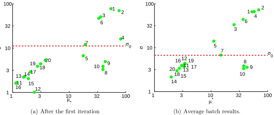
135
compared with (1) which is optimal for computing elementary effects, see Pujol (2009).
136
4
Sequential elementary effects method
137
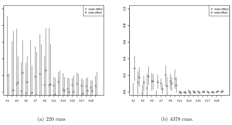
We propose a sequential screening method that has the potential to reduce computation time
138
significantly. The methodology aims to distinguish between factors with linear or no effect
139
and factors with non-linear effect. In the EE method, all (k+ 1) evaluations are performed
140
for each trajectory irrespective of the type of factor effect. Whereas, in our sequential
141
strategy, when effects are identified as non-linear, their corresponding one-step evaluations
142
are removed from subsequent trajectories. This results in fewer model runs. The rationale
143
is that if σi is small for a given factor, then we should investigate whether σi remains small 144
when adding extra trajectories. At the end of experimentation, those input factors for which
145
σi remained small are considered to have linear or no effect, and factors for which σi was 146
bigger than a threshold have a non-linear effect on the output. A method of eliciting the
147
choice of threshold is presented in Section 4.1.
148
The justification of thresholding solely on the variance of the elementary effects σi is 149
that independent linear effects of factors may be removed from the simulator output at a
150
preprocessing stage or during the emulation phase. As an example of the latter approach,
151
factors with linear effects may be incorporated in the mean function of a Gaussian Process
152
(GP) emulator while omitted from the covariance specification. If we denote by A the
153
subset of {1, . . . , k} that indexes factors with linear effects, the GP prior may be written
154
as Y(x) =β+Pk
i=1aiXi+Z∗ where Z∗ is a stochastic process whose covariance structure 155
depends only on the variables with non-linear effects; that is, the xi withi∈ {1, . . . , k} \A. 156
The residual process Z∗ is therefore placed in a lower dimensional space simplifying the 157
design and inference tasks.
158
For our algorithm to run, a space filling design with M points is created. This design
159
provides the sequence of points at which the Morris OAT runs will be tested. Initially, we
160
select a good space filling design, such as a maximin Latin hypercube (LH) (Morris and
161
Mitchell, 1995). The generation of maximin designs is discussed further in (Ravi et al.,
162
1994). The value of M is selected such that (k+ 1)M is the maximum number of runs that
can be performed during the whole screening process.
164
A preprocessing stage orders the design points according to the biggest distance between
165
points. The first two points are those whose Euclidean distance is largest; then the third
166
point maximises the minimum distance between itself and the first two points, then a fourth
167
point is ordered in the same way, and so on. This procedure of ordering points mirrors
168
nearest neighbour clustering, but acts in an opposite manner as points are ordered from
169
those farthest apart to those that are closest.
170
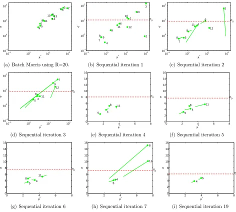
Example 1. For k = 5 input factors and M = 6 runs, consider a maximin LH design in
171
[0,1]5 with point coordinates x
1 = (0,4,1,4,4)/5, x2 = (1,5,5,1,3)/5, x3 = (2,1,3,0,1)/5,
172
x4 = (3,0,4,5,2)/5, x5 = (4,3,0,3,0)/5 and lastly x6 = (5,2,2,2,5)/5. The preprocessing
173
stage first selects the points x2 and x5, which are furthest apart. The next point, x4,
174
maximises the distance between those remaining points and the first two points chosen.
175
The procedure continues by selecting x6, then x1 and finishes with x3. This preprocessing
176
stage produces the ordered sequence of points x2,x5,x4,x6,x1,x3, which are relabelled as
177
x(1), . . . ,x(6).
178
The screening algorithm starts with the computation of elementary effects for all input
179
factors at the first two design points of the ordered maximin LH design. OAT runs are
180
created at those two points and elementary effects are computed. With this initial data,
181
a first estimation of the moments µi, µ∗i and σi is available. If, for a given input factor, 182
its sample moment σi is larger than a specified threshold σ0, then we say that the output
183
is responding non-linearly to this input. This leads us to declare that input as active and
184
remove it from the list of current input factors. The technique continues by adding OAT runs
185
at the next point, only for factors suspected to be linear. Elementary effects are computed
186
and moments are updated for each added point, removing a factor if the condition for σi is 187
met. The methodology ends when all input factors have been removed or after computing
188
elementary effects for all M points. On ending, the input factors are separated into two
189
groups: those having non-linear effect and those with linear or no effect on the output.
190
Algorithm 1 sets out the procedure in pseudo-code form.
191
Example 2. To show how the proposed sequential algorithm works, considerY(x1, x2, x3, x4, x5) =
192
cos(x3/5)(x2+ 1/2)4/(x1+ 1/2)2+x5 on the design region [0,1]5. Note that x4 has negligible
Algorithm 1 The procedure for completing our screening technique.
Screening algorithm
Input: Simulator Y(·) with k inputs; total number of one-at-a-time experi-ments M; step size ∆; threshold σ0.
Output: Moments µi, σi, µ∗i; lists of factors with linear (C) and with
non-linear effect (A).
A.Preprocessing stage
1. Set design region to [0,1]k and create space filling design with M points
x1, . . . ,xM.
2. Order the design points using maximum distance between points. Label the ordered points asx(1), . . . ,x(M).
B.Calculating the elementary effects
1. Set R:= 2 and the initial design to beD:=
x(1),x(2) . Set list of current
factors toC:={1, . . . , k}and list of active effects A:=∅.
2. For every point in D, create one-at-a-time runs only for those input fac-tors indexed by C. Run the simulator at those points. This totals |C|+ 1 experiments for every point inD.
3. Using simulator runs from step B2 and (1), compute elementary effects
{EEi(x) :x∈D, i∈ C}.
4. If R = 2, compute moments µi, µ∗
i and σi using elementary effects for all
factors. IfR >2, only update moments for the current list of input factors, indexed byC.
5. For i∈ C, ifσi> σ0 then update C:=C \ {i} and A:=A ∪ {i}.
6. If C=∅, then all the inputs were identified non-linear. Algorithm ends.
7. If R = M, then all the design points available are exhausted. Algorithm ends.
C. Producing the next design point
1. Update R:=R+1; set D={x(R)}.
effect here. The function Y is treated as a simulator, from which the only information we
194
require are its values at design points. We use the same pre-ordered LH design of Example
195
1; set p= 10 for step size ∆ = 5/9 and threshold σ0 = 0.15. See 4.1 for details on the
con-196
struction of the threshold σ0. Random trajectories are constructed with the first two ordered
197
points, giving the following moment estimates (µ1, µ2, µ3, µ4, µ5) = (−7.87,4.66,−0.047,0,1)
198
and (σ1, σ2, σ3, σ4, σ5) = (6.62,0.27,0.06,0,0). Note that the method yields exact zeroes for
199
the fourth variable. The estimates σ1, σ2 are greater than the threshold σ0 and thus x1
200
and x2 are separated as having non-linear effects. As all σ3, σ4 and σ5 are smaller than
201
σ0, further investigation is required for x3, x4 and x5. At the third design point, OAT
ex-202
perimentation only for those factors produces updated moments (µ3, µ4, µ5) = (−0.06,0,1)
203
and (σ3, σ4, σ5) = (0.05,0,0), i.e. the factors remain under investigation. The sequential
204
methodology continues for all of them until finishing with all the design points. At this final
205
step, updated moments are (µ3, µ4, µ5) = (−0.039,0,1) and (σ3, σ4, σ5) = (0.04,0,0), where
206
again for the fourth factor the results are exactly zero. We conclude that linearity of the
207
response in terms of x3, x4 and x5 over the design region could not be rejected. Near zero
208
variances for x4 and x5 suggest strong conclusions for those factors.
209
The total experimental effort was 28 runs, from which the first 12 runs involved
tra-210
jectories for all factors, while further 16 runs were required for the linear factors under
211
investigation. This is a 22% reduction from the (5 + 1)∗6 = 36 runs needed to perform the
212
batch EE method. The moment estimates obtained for the non-linear factors are only rough
213
approximations of the true moment values, and the moment estimates for the linear factor
214
were computed with more information. This asymmetry is apparent when comparing with
215
exact analytic sensitivity results µ= (−5.34,6.62,−0.04,0,1) andσ = (8.88,7.42,0.06,0,0),
216
where we use µi =
R [0,1]5
∂
∂xiY(x)dxand σ
2
i =
R [0,1]5
µi−∂x∂iY(x)
2
dx.
217
4.1
Heuristic selection of variance threshold
218
In Algorithm 1, the elementary effect variance threshold σ0 is an input. In this section, we
219
present a heuristic to chooseσ0 indirectly by eliciting the expected divergence from linearity
220
of the factor effect as the variance of an auxiliary random variable. A linear (or near-linear)
effect of the variable xi is represented by an additive noise model: 222
Y(xi) =axi +b+εi, (3)
where εi is an independent and identically distributed normal random variable with zero 223
mean and known variance γ, and a, bare constants. In other words, the marginal effect due
224
to the factor xi is modelled with a simple regression line. The auxiliary random variable εi 225
captures interaction with other factors and non-linearities.
226
In practice, the variance γ has to be elicited prior to the screening experiment and there
227
are two alternatives that we have considered in the examples in the present paper.
228
1. We might believe that the factorxi has a linear effect, but the simulator runs contain a 229
numerical error. In this case, we expect γ to be set to a small value, such as a multiple
230
of machine precision.
231
2. If we believe that small non-linear effects will not have an appreciable impact on the
232
model output, then γ should be chosen to reflect the level of variation from a straight
233
line to be tolerated.
234
The elicitation of the variance parameter is in contrast to Kadane et al. (1980) and
235
Garthwaite and Dickey (1988), where full probability distributions are elicited that reflect
236
beliefs about the parameters of the linear model. In the present application, we do not wish
237
to prejudge the behaviour of the model: we want a number specifying how far we can tolerate
238
from being linear.
239
Given the varianceγ, the sampling distribution of the variance of the elementary effects
240
can be calculated according to the following lemma, whose proof is given in Appendix A.
241
For simplicity we omit the subscriptifrom the quantitiesσ2,σΦ,γ and ∆, all of which could
242
potentially take different values for each input. In practice we choose a common γ and ∆
243
for all inputs.
244
Lemma 1. Let x1, . . . , xR be univariate design points, at each of which trajectories are 245
constructed. Assume that observations taken at design points and trajectories follow the
246
model given in (3). Let elementary effects and moments be defined as in (1) and (2) and let
σ2 Φ = 2
γ
∆2. Then
248
σ2 ∼ σ
2 Φ
R−1χ
2
R−1. (4)
where χ2
R−1 denotes a chi-square random variable with R−1 degrees of freedom. 249
We propose to use the 99% quantile of the cumulative distribution function of the
chi-square distribution to derive the EE variance threshold σ0. We have found this choice
of quantile sufficiently conservative for the examples we have investigated. The following
equation
P σ2 ≤σ20
=P
σ2 Φ
R−1χ
2
R−1 ≤σ
2 0
= 0.99,
when inverted yields the threshold
250
σ0 = q
χ2
0.99,R−1σ2Φ/(R−1), (5)
whereχ2
0.99,R−1is the 99% quantile of a chi-squared distribution withR−1 degrees of freedom.
251
In other words, σ0defines a threshold over which the effect is considered non-linear; that is, if
252
σi < σ0, then the input variablexi is retained for further testing. Note that Lemma 1 applies 253
directly in a multivariate setting; in which case, the comparison is performed separately for
254
each input variable.
255
In Example 2, we used a single thresholdσ0 for all variables. In order to obtainσ0 = 0.385
256
using the method described in this section, the values R= 6, ∆ = 5/9,√γ = 8.7×10⁻² and 257
quantile χ2
0.99,5 = 15.08 could be used.
258
To simplify the algorithm, the thresholdσ0 may be kept fixed for all computations rather
259
than adapting σ0 to the actual number of trajectories involved. The main difference is in
260
the degrees of freedom for the scaled chi-square distribution in (5). The adaptive approach,
261
which was utilised in the simulation experiments presented, involves recomputing σ0 with
262
updated degrees of freedom prior to step B5 in Algorithm 1. In the simplified approach using
263
a single value σ0, the method is more conservative than when varying degrees of freedom;
264
i.e. the rejection rate is higher with fixed threshold than otherwise.
265
The detection of nonlinearity under the heuristics in this section is further explored in
266
Appendix B. The robustness of the proposed selection of σ0 in our sequential algorithm is
267
explored under different departures from linear model (3).
5
Simulated high dimensional example
269
We illustrate the sequential screening method on the synthetic test function introduced in
270
Morris (1991). The function is defined on 20 inputs x∈[0,1]20 as follows:
271
y=β0+ 20 X
i=1
βiwi+
20 X
i<j
βijwiwj +
20 X
i<j<l
βijlwiwjwl+
20 X
i<j<l<s
βijlswiwjwlws, (6)
where wi = 2(xi − 12) except for i = 3,5,7 where wi = 2 1.1xi/(xi+ 0.1)−12
. The
coef-272
ficients are set to βi = 20 for i = 1, . . . ,10, βij = −15 for i, j = 1, . . . ,6, βijl = −10 for 273
i, j, l = 1, . . . ,5 and βijls = 5 for i, j, l, s = 1, . . . ,4. The remaining first and second order 274
coefficients are generated independently from a zero mean unit variance normal distribution
275
and the remaining third and fourth order coefficients are set to zero. Factors x1, . . . , x7 have
276
a non-linear effect on the function output while factors x8, x9, x10 have a linear effect and
277
factors x11, . . . , x20 have negligible effect (Morris, 1991; Pujol, 2009).
278
First, we compare the performance of the batch and sequential EE methods in terms of
279
required model runs. The screening experiment was performed under the configuration used
280
in Pujol (2009) for 100 realisations. As in Pujol (2009) the discretisation level has been set
281
to p = 20 so ∆ = 0.5263 and the number of trajectories to R = 10. For the sequential
282
procedure, a threshold value of γ= 2.6 was used. This corresponds to around 0.005% of the
283
range of the response y in (6), which varies between −225 and 139.
284
A total of 210 function evaluations are required for the batch EE procedure. For the
285
sequential EE procedure on average 150 function evaluations are required with a standard
286
deviation of 13, that is an average savings of 28% compared to the batch approach. Factors
287
x1, . . . , x7are correctly identified as having non-linear effect in 99% of the realisations because
288
the corresponding σi is larger than the threshold σ0. Factors x8, . . . , x10 are found to have
289
linear effects in 92% of the realisations becauseµiis large andσi is small. Factorsx11, . . . , x20
290
are found to have negligible in all realisations due to small σi values. The full batch EE 291
screening results and the first iteration of one realisation of the sequential algorithm are
292
shown in Figure 1. This first iteration is equivalent to running the algorithm up to step B.4
293
in Algorithm 1. We note that six of the seven factors with non-linear effects are identified
294
at this early stage.
1 3 10 32 100 1
3 10 32 100
1 2 3
4
5 6
7
8 9 10
11 12 13 14
15 16
17 18 19 20
σ0
µ*
σ
(a) After the first iteration
1 3 10 32 100 1
3 10 32 100
1 2
3
4
5
6
7
8 9 10 11
12 13 14
15 16
17 18
19 20
σ0
µ*
σ
[image:14.595.69.536.68.265.2](b) Average batch results.
Figure 1: Applying the batch and sequential EE screening method on the 20 input factor Morris test function. Horizontal dashed line denotes the σ0 threshold value for the given
iteration.
Finally, we illustrate the efficiency of the EE method by contrasting it to a traditional
296
sensitivity analysis method. Applying the Sobol’ sensitivity analysis method (Sobol, 1993) to
297
compute first-order and total indices using a random design of 220 runs, results in large 95%
298
confidence intervals indicating that more model runs are required before any conclusions can
299
be drawn from the examination of the indices (Figure 2). We also show how the uncertainties
300
dramatically reduce when a larger design is used. These results were obtained by using the
301
sensitivity R package (Pujol et al., 2013). This illustration confirms our expectation that
302
screening methods such as the EE method, can be utilised prior to a more detailed sensitivity
303
analysis in order to minimise the number of model runs.
304
We conclude that the sequential approach results in significant computational savings
305
compared to the batch EE method as factors with clear non-linear effects can be eliminated
306
in the early screening stages with high confidence. Furthermore, we have demonstrated the
307
efficiency of the EE screening methods compared to classical sensitivity analysis as illustrated
308
by the number of runs required to effectively calculate the Sobol’s first-order and total indices
309
for this example.
X1 X3 X5 X7 X9 X11 X13 X15 X17 X19
0.0
0.2
0.4
0.6
0.8
1.0
0.0
0.2
0.4
0.6
0.8
1.0 main effect
total effect
(a) 220 runs
X1 X3 X5 X7 X9 X11 X13 X15 X17 X19
0.0
0.2
0.4
0.6
0.8
1.0
0.0
0.2
0.4
0.6
0.8
1.0 main effect
total effect
[image:15.595.81.527.85.325.2](b) 4378 runs.
Figure 2: Applying Sobol’s sensitivity analysis method on data generated using (6). Random designs of 220 and 4378 have been used. The error bars indicate 95% confidence intervals for the first-order and total effect indices.
6
Rabies Model
311
In this section, we discuss the application of the Morris sequential screening method described
312
in Section 4 on a stochastic model provided by the Food and Environment Research Agency
313
(FERA) (Singer et al., 2008, 2009). An overview of the stochastic simulator is given in
314
Section 6.1, followed by a description of the screening methodology in Section 6.2) and a
315
discussion of the results in Section 6.3.
316
6.1
Model Description
317
Although rabies in wild animal populations has been eradicated from large parts of Europe,
318
there is a remaining risk of disease re-introduction. The situation is aggravated by an
319
invasive species, the raccoon dog (Nyctereutes procyonoides) that can act as a second rabies
320
vector in addition to the red fox (Vulpes vulpes). The purpose of the rabies model is to
321
analyse the risk of rabies spread in this new type of vector community (Singer et al., 2008).
322
The individual-based, non-spatial, discrete-time model incorporates population and disease
dynamical processes such as host reproduction and mortality as well as disease transmission.
324
The model includes two vector species: raccoon dogs and foxes. The model is non-spatial
325
and disease propagation is calculated solely with respect to population dynamics.
326
Description min max 1 Number of replications 200 300 2 Fox population winter density (ind./km2) 0.1 0.5 3 Raccoon dog population winter density (ind./km2) 0.1 1 4 Shape parameter for the probability distribution 0.39 0.47
of raccoon dog infection
[image:16.595.120.461.137.351.2]5 Dummy variable with no influence 0.9 1.1 6 Fox population mortality 0.9 1.1 7 Raccoon dog population mortality 0.9 1.1 8 Winter hunting proportion 0.9 1.1 9 Fox population birth rate 0.9 1.1 10 Raccoon dog population birth rate 0.9 1.1 11 Fox population infection rate 0.9 1.1 12 Fox population rabies incubation rate 0.95 1.05 13 Raccoon dog rabies incubation rate 0.95 1.05
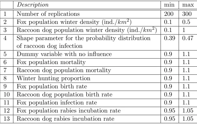
Table 1: Input parameters for the rabies model and their ranges.
The model has 13 free parameters, shown in Table 1. In addition, three simulator
config-327
uration parameters were kept fixed: the maximum number of time steps was set to 400; the
328
cross infection input was 0.002 and the environment area size was kept fixed at 5400 km2.
329
The response used is the probability that the rabies disease becomes extinct in both
330
species within 5 years. This output is scaled to lie in the range [0,100] and is important
331
in deciding on the response to a potential rabies outbreak since it indicates the risk of long
332
term rabies disease persistence (Singer et al., 2008, 2009).
333
6.2
Screening Methodology
334
For screening, we utilise a Morris design with the number of trajectories set to R = 20
335
resulting in (k + 1)×R = 14×20 = 280 simulator evaluations, where k = 13. The mean
336
µ∗ of the absolute values of the Elementary Effects is used to rank the input factors. We set 337
the number of levels to p= 6 and ∆ =p/(2(p−1)) = 0.6.
338
The sequential Morris method discussed in Section 4 allows the specification of a variance
339
γ from which the threshold on the Elementary Effect deviationσ0is derived. We setγ = 3.5,
which reflects a prior belief that individual factor effects on the output are considered
near-341
linear if the effect on the output is within three standard deviations of purely linear, i.e.
342
±3√γ = 5.6. Since the output is bounded in the range [0,100] a factor has near-linear effect
343
if the output varies no more than 5.6% from linear. This variability encapsulates both the
344
internal variability of the stochastic model and our prior definition of a near-linear effect.
345
6.3
Screening Results
346
Singer and Kennedy (2008) performed sensitivity analysis on this model using the standard
347
Morris method with the same setup as here as well as the Sobol’ method. They noted the
348
most important parameters are species winter densities (inputs (2) and (3)) and mortalities
349
(inputs (6) and (7)). They also noted the least influential factors are the dummy variable (5)
350
that has by definition no influence on the model output and parameter 4, a shape parameter
351
for the probability distribution of raccoon dog infection. It is also noted that the Sobol’
352
method is prohibitively expensive and offers low accuracy with a sample size of 300. They
353
suggested increasing the sample size and reducing the dimensionality of the problem by
354
fixing some of the factors to their nominal values. For expensive simulators this motivates
355
the usage of the Morris method.
356
The standard Morris method variable ranking with R = 20 trajectories is presented in
357
Figure 3(a) where the four dominant factors were found to be the winter densities for both
358
species (2,3) and the associated mortality rates (6,7). Singer and Kennedy (2008) have noted
359
that the dominant factors have strong non-linear and interaction effects which is reflected in
360
the high σ value observed in the Morris method.
361
The sequential Morris method is initialised with R = 2 trajectories on all 13 factors
362
requiring (k+ 1)R = 28 simulator runs. The same step size ∆ and the computed threshold
363
σ0 is the same for all factors. The Morris plot with the associated threshold value is shown
364
in Figure 3(b). The elementary effect variance is over the threshold for four factors, the
365
raccoon dog winter density (3), raccoon dog rabies incubation probability (13), number of
366
replicated runs (1) and raccoon dog population birth rate (10) are eliminated from further
367
consideration since they have strong non-linear effects on the simulator output.
368
Another trajectory design for the remaining 9 factors is evaluated and requires 10 further
369
simulator evaluations (Figure 3(c)). The parameters fox winter density (2) and mortality
(6) factors are found to have non-linear effects and are removed from further consideration.
371
As evidenced by the Morris plot, the σ value for parameter 2 changed significantly from the
372
previous iteration where the effect was considerably below the threshold and very close to
373
linear.
374
For the third iteration, the seven factor trajectory requires 8 more simulator evaluations
375
(Figure 3(d)). Three further parameters are eliminated, the raccoon dog (7) mortality rate,
376
the fox birth rate (9) and the fox population rabies incubation probability (12) where large
377
changes in the moments of the elementary effects are again observed due to the increased
378
accuracy from the increased Morris design size. No more factors are eliminated until iteration
379
7 requiring a further (4 + 1)×4 = 20 simulator evaluations (Figure 3 (e)-(h)). At iteration
380
7, the winter hunting proportion (8) and fox population infection rate (11) parameters are
381
removed from further consideration.
382
The remaining two factors, the shape parameter for the probability distribution (4) and
383
the dummy variable (5), are found to be below the σ threshold for all subsequent twelve
384
iterations requiring (2 + 1)12 = 36 simulator evaluations. The total number of simulator
385
evaluations for the sequential procedure is 102 compared to the 280 evaluations required by
386
the standard batch Morris method with R = 20 trajectories, yielding a 27% reduction in
387
required code runs.
388
We have also performed the threshold calculation on the full Morris set with R = 20
389
trajectories and the same factors as with the sequential version are identified as near-linear.
390
In summary, the sequential Morris method for the rabies model has been successfully used
391
to identify factors with no or near-linear effects on the simulator response at a significant
392
saving to the standard Morris method.
393
7
Discussion
394
We have presented a novel sequential screening method that extends the batch elementary
ef-395
fects method originally proposed by Morris (1991). The method aims to identify inputs with
396
non-linear effects with a minimum number of trajectories. We have empirically demonstrated
397
the computational savings achieved compared to the batch approach on both synthetic data
398
and a real-world simulator. A critical aspect of the method is the specification of the
10−1 100 101 102 10−1 100 101 102 1 2 3 45 6 7 8 9 10 11 12 13 σ µ*
(a) Batch Morris using R=20.
10−1 100 101 102
10−1 100 101 102 1 2 3 4 5 6 7 8 9 10 11 12 13 σ0 σ µ*
(b) Sequential iteration 1
10−1 100 101 102
10−1 100 101 102 2 4 5 6 7 8 9 11 12 σ0 σ µ*
(c) Sequential iteration 2
10−1 100 101 102
10−1 100 101 102 4 5 7 8 9 11 12 σ0 σ µ*
(d) Sequential iteration 3
0 2 4 6 8
0 2 4 6 8 10 12 14 16 4 5 8 11 σ0 σ µ*
(e) Sequential iteration 4
0 2 4 6 8
0 2 4 6 8 10 12 14 16 4 5 8 11 σ0 σ µ*
(f) Sequential iteration 5
0 2 4 6 8
0 2 4 6 8 10 12 14 16 4 5 8 11 σ0 σ µ*
(g) Sequential iteration 6
0 2 4 6 8
0 2 4 6 8 10 12 14 16 4 5 8 11 σ0 σ µ*
(h) Sequential iteration 7
0 2 4 6 8
0 2 4 6 8 10 12 14 16 4 5 σ0 σ µ*
[image:19.595.64.536.154.578.2](i) Sequential iteration 19
Figure 3: Batch and Sequential EE screening on the rabies simulator. Solid line denotes path from previous value of (µ∗, σ) for each factor. Horizontal dashed line denotes the σ
0
old σ0 which is used to determine whether an input has a non-linear effect. The elicitation
400
of this value directly can be challenging and we have presented an indirect approach which
401
utilises an easily interpetable variance value γ specified on the simulator output space.
402
In order to apply the screening method of the present paper, the analyst must make a
403
number of choices. To create the ordered design of OAT-experiment start-points,M must be
404
specified. We recommend that M is chosen with respect to the computational effort needed
405
to run the simulator; at worst, the simulator will run (k+ 1)M times. The threshold valueσ0
406
can be set to zero so that only true linear- and no-effect inputs are investigated. We suggest
407
to use a threshold σ0 > 0 as in practice some small non-linearities might be tolerated and
408
replaced instead by a linear function.
409
In cases where direct elicitation of the EE variance thresholdσ0 is not feasible or
straight-410
forward, elicitation of the variance γ may be preferable. The varianceγ may be interpreted
411
as the expected divergence of a factor from strict linearity under which the factor effect may
412
still be considered linear for modelling purposes. In the case of stochastic simulators, this
413
parameter includes the internal simulator variability whereas for deterministic simulators
414
near-linear definitions only include errors due to machine precision and degree of departure
415
from truly linear effects on the output. In the future, alternative elicitation methods may be
416
constructed to allow for other non-Gaussian deviations from linear effect. An area of future
417
interest is double classification of factors using the joint distribution of moments µ∗
i and σi.
418
This not only would classify a factor as linear or non-linear, but would discriminate between
419
active and non-active factors. A starting point for this would be the t test for µ in Morris
420
(1991).
421
A variation of our algorithm is to select OAT runs to improve space filling properties of
422
the whole design. The simplest approach is to use random OAT runs. However, OAT runs
423
can be selected to maximise distance between them, as in Campolongo et al. (2007). An
424
adaptation of the OAT runs suggested in Pujol (2009) can also be used where we create a
425
simplex in the current set of input factors. Another criterion is to select OAT runs to improve
426
uniformity of unidimensional projections of the design thus minimising the unidimensional
427
discrepancy of the whole design, conditioned on the initial hypercube. The use of discrepancy
428
to measure uniformity stems from quasi-Monte-Carlo methods (Niederreiter, 1992). We
429
have used Sobol’s low discrepancy space filling sequence (Niederreiter, 1992). The only
change required in the pseudo-code of Algorithm 1 is to remove step A2. Sampling from low
431
discrepancy sequences has the advantage of sequential generation of points. However, for
432
small sample sizes the spread of points of a low discrepancy sequence may not be as good as
433
that of a maximin space filling design with fixed size.
434
In this paper, we have not addressed the question of how multiple simulator outputs could
435
be handled in our method. The simplest approach, of generating separate OAT designs for
436
each output, is inefficient. In a sequential setting, the initial design could be shared for all
437
outputs. In our approach, factors are excluded from subsequent screening stages when
non-438
linear effects are detected. Therefore, subsequent stages need only include factors that are
439
under the EE variance threshold across all outputs. As the number of outputs grows, it is
440
more likely that a factor will have a non-linear effect on at least one of the outputs. Therefore
441
fewer simulator runs will be required for screening but it is also more likely fewer factors with
442
only linear or no effects across all outputs are detected. An alternative approach would be to
443
use a functional summary of all simulator outputs as the response for the screening analysis.
444
However the EE variance threshold will need to be elicited for the functional summary rather
445
than for each individual simulator output.
446
Acknowledgements
447
This work was carried out within the Managing Uncertainty in Complex Models (EPSRC
448
grant EP/D048893/1). We thank Dan Cornford for many useful discussions. We also thank
449
Graham Smith and Alexander Singer at the Food and Environment Research Agency for
450
providing the rabies model and explaining the simulator structure.
451
A
Proof of Lemma 1.
452
Proof. All computations in this lemma are defined for a single factor. The elementary effect
453
at point xi follows a normal distribution EE(xi) ∼ N(a,∆2γ2). Independence of elementary
454
effects EE(x1), . . . , EE(xR) follows from independence of observations of model. 455
The mean ofR elementary effects is distributed µ∼N(a,R2∆γ2). To find the distribution
of σ2 = 1
R−1
PR
i=1(EE(xi)−µ)2, the following sum of squares is used 457
R
X
i=1
EE(xi)−a
q 2γ
∆2
2
= (R−1)σ
2
2γ
∆2
+R(µ−a)
2
2γ
∆2
.
The left hand side above is a sum of squared independent standard normal variables and
458
thus it has a chi-squared distribution with R degrees of freedom. By independence of µ
459
and σ2, the first summand on the right has a chi-squared distribution with R−1 degrees of
460
freedom and the second summand has a chi-squared distribution with one degree of freedom.
461
Therefore σ2 ∼ 2γ
(R−1)∆2χ2R−1.
462
B
Power computations
463
The input xi is declared non-linear the first time that σi satisfies σi > σ0 in step B5 of the
464
algorithm. If the total number of experiments satisfiesM > 2, then detection of nonlinearity
465
for a given input can occur before the total number of allowed experiments M is reached.
466
Power computations are possible for different departures from the linear model used to
467
determine σ0, here we explore two.
468
The first departure we consider is a change in variance, with varianceγ being multiplied
469
by a factorδ2to becomeγ′ =δ2γ. The factorδquantifies change in variance from the original
470
model. The probability of detecting the change at the step R is Pr X2
R−1 > χ20.99,R−1/δ2
.
471
A geometric walk argument with probabilities changing as more data is included yields the
472
power: 1−QM
R=2 1−Pr XR2−1 > χ20.99,R−1/δ2
.
473
A different departure from linear model is when data follows
474
Y(xi) =cx2i +axi+b+εi. (7)
Hereεistill satisfies the same assumptions as for the linear model anda, bandcare constants. 475
The following scenarios were used for power computations through simulations under the
476
(wrong) model (7): M = 2,3,4,5, a = 101,15,12,1; and the quadratic coefficient depended
477
on the slope through the following relation c = δa with δ ranging from 10−2 to 103. Here 478
the quantity δ is used to quantify departures from the original model through an increasing
1 5 10 50 500
0.01
0.05
0.20
0.50
delta
po
w
er
M=2 M=3
M=4 M=5
1 5 10 50 500
3.0
3.5
4.0
4.5
5.0
delta
ARL
a=1 0.5
0.2 a=0.1
[image:23.595.165.418.72.217.2](a) (b)
Figure 4: Simulation results: (a) power and (b) ARL against scaling factor δ.
quadratic coefficient. The errors in the models simulated were standard normal, i.e. γ = 1
480
and in each scenario used a uniform design of M points over [0,1]. The results of power
481
against different values of M with a= 101 are shown in Figure 4 (a). As would be expected,
482
the test reacts quickly to increasing quadratic trend through δ, but also asM increases and
483
even for very small changes there is already a higher rejection rate. For instance, when
484
M = 5 the rate is already larger than 10%.
485
In each simulation experiment, the run length was recorded. Recall that run length is the
486
number of steps required for a factor to be declared nonlinear and it only takes integer values.
487
A number of 12,000 simulations were carried out and run lengths obtined were averaged to
488
produce the average run length (ARL). This computation was performed for M = 5 and
489
same scenarios for parameters a and c as above. The graph of ARL against δ is shown in
490
Figure 4 (b), where the top curve (a = 101 ) required more exploration and produced higher
491
ARL than the rest of the cases for a, with the lowest ARL in the simulations achieved for
492
a = 1 (bottom curve), where the departure from linear is highest and the method detects it
493
very quickly. Simulations for both Figures 4 (a) and (b) used the same range ofδ but in the
494
right figure the results are plotted only for M = 5.
495
Supplementary Materials
496
Technical Report: Supplementary information on the scalability of the sequential
elemen-497
tary effects method. (pdf)
Matlab code for the sequential screening method: Matlab code that demonstrates the
499
sequential screening method on a synthetic dataset. The example can be started by
500
running seqMorrisExample.m. (GNU zipped tar file)
501
References
502
Andres, T. (1997). Sampling methods and sensitivity analysis for large parameter sets.
503
Journal of Statistical Computation and Simulation, 57(1-4):77–110.
504
Campolongo, F. and Braddock, R. (1999). The use of graph theory in the sensitivity analysis
505
of the model output: a second order screening method. Reliability Engineering & System
506
Safety, 64(1):1–12.
507
Campolongo, F., Cariboni, J., and Saltelli, A. (2007). An effective screening design for
508
sensitivity analysis of large models. Environmental Modelling Software, 22(10):1509–18.
509
Campolongo, F., Cariboni, J., Saltelli, A., and Schoutens, W. (2004). Enhancing the Morris
510
Method. In Hanson, K. M. and Hemez, F. M., editors,Proceedings of the 4th International
511
Conference on Sensitivity Analysis of Model Output, pages 369–79, Santa Fe, New Mexico.
512
Cukier, R., Fortuin, C., Shuler, K., Petschek, A., and Schaibly, J. (1973). Study of the
513
sensitivity of coupled reaction systems to uncertainties in ratecoefficients. Journal of
514
Chemical Physics, 59:38733878.
515
Garthwaite, P. H. and Dickey, J. M. (1988). Quantifying expert opinion in linear regression
516
problems.Journal of the Royal Statistical Society. Series B. Methodological, 50(3):462–474.
517
Hargreaves, J. C., Annan, J. D., Edwards, N. R., and Marsh, R. (2004). An efficient
cli-518
mate forecasting method using an intermediate complexity Earth System Model and the
519
ensemble Kalman filter. Climate Dynamics, 23:745–60.
520
Kadane, J. B., Dickey, J. M., Winkler, R. L., Smith, W. S., and Peters, S. C. (1980).
521
Interactive elicitation of opinion for a normal linear model. Journal of the American
522
Statistical Association, 75(372):845–854.
Kennedy, M., Anderson, C., O’Hagan, A., Lomas, M., Woodward, F., Gosling, J., and
524
Heinemeyer, A. (2008). Quantifying uncertainty in the biospheric carbon flux for England
525
and Wales. Journal of the Royal Statistical Society - Series A, 171:109–135.
526
Kleijnen, J. P. C. (2009). Factor screening in simulation experiments: Review of sequential
527
bifurcation. Advancing the Frontiers of Simulation: A Festschrift in Honor of George S.
528
Fishman, pages 147–173.
529
Linkletter, Crystal, Bingham, Derek, Hengartner, Nicholas, Higdon, David, Ye, and Kenny,
530
Q. (2006). Variable selection for gaussian process models in computer experiments.
Tech-531
nometrics, 48(4):478–490.
532
Morris, M. and Mitchell, T. (1995). Exploratory designs for computer experiments. Journal
533
of Statistical Planning and Inference, 43:381–402.
534
Morris, M. D. (1991). Factorial sampling plans for preliminary computational experiments.
535
Technometrics, 33:161–74.
536
Niederreiter, H. (1992).Random number generation and quasi-Monte Carlo methods. Society
537
for Industrial and Applied Mathematics, Philadelphia, PA, USA.
538
O’Hagan, A. (2006). Bayesian analysis of computer code outputs: a tutorial. Reliability
539
Engineering & System Safety, 91:1290–1300.
540
Pujol, G. (2009). Simplex-based screening designs for estimating metamodels. Reliability
541
Engineering & System Safety, 94:1156–60.
542
Pujol, G., Iooss, B., and Janon, A. (2013). sensitivity: Sensitivity Analysis. R package
543
version 1.7.
544
Ravi, S. S., Rosenkrantz, D. J., and Tayi, G. K. (1994). Heuristic and special case algorithms
545
for dispersion problems. Operations Research, 42(2):pp. 299–310.
546
Reich, B. J., Storlie, C. B., and Bondell, H. D. (2009). Variable selection in bayesian
smooth-547
ing spline anova models: Application to deterministic computer codes. Technometrics,
548
51(2):110–120.
Sacks, J., Welch, W., Mitchell, T., and Wynn, H. (1989). Design and analysis of computer
550
experiments. Statistical Science, 4:409–23.
551
Saltelli, A., Chan, K., and Scott, E., editors (2000). Sensitivity Analysis. New York: Wiley.
552
Savitsky, T., Vannucci, M., and Sha, N. (2011). Variable Selection for Nonparametric
Gaus-553
sian Process Priors: Models and Computational Strategies. ArXiv e-prints.
554
Singer, A., Kauhala, F., Holmala, K., and Smith, G. (2008). Towards the elimination of
555
rabies in eurasia. Developments in Biologicals, 131:213–222.
556
Singer, A., Kauhala, F., Holmala, K., and Smith, G. (2009). Rabies in northeastern europe
557
- the threat from invasive raccoon dogs. Journal of Wildlife Diseases., 45(4):1121–1137.
558
Singer, A. and Kennedy, M. (2008). Sensitivity analysis on the rabies model. Personal
559
Communication.
560
Sobol, I. M. (1993). Sensitivity analysis for non-linear mathematical models. Math. Modelling
561
Comput. Exp., 1:407–414.
562
Wedge, D. C., Rowe, W., Kell, D. B., and Knowles, J. (2009). In silico modelling of
di-563
rected evolution: Implications for experimental design and stepwise evolution. Journal of
564
Theoretical Biology, 257:131–41.