Robust dimensional variation control of compliant assemblies through the application of sheet metal joining process sequencing

(1)

Robust dimensional variation control of

compliant assemblies through the

application of sheet metal joining process

sequencing

Adam Nagy-Sochacki

October 2015

A thesis submitted for the degree of

Doctor of Philosophy

of

The Australian National University

c

(2)

(3)

Acknowledgments

This has been a long journey for me, and without a doubt has taken me further than

I thought possible. I would never have gotten to the end without a strong group of

people around me, helping in many different ways.

Firstly, I would like to thank my supervisors, Doctor Matthew Doolan, Professor

Michael Cardew-Hall and Associate Professor Bernard Rolfe. It has been a long battle

to get to the end and they have given me nothing but encouragement and support.

They never gave up on me, and exhibited patience beyond comprehension. I think

this was quintessential to getting to the end, and it is a trait I admire greatly.

My sincerest thanks to Ford Australia for their support with this project and to all

those that were involved in my time down in the factory in Geelong; including the

technical inspection team at the time Peter Jenkinson, Chris Wickens, Andrew Hill,

Glen Rush and Peter Ilijevski.

All the past and current research students that have gone through the Materials

and Manufacturing research group; in particular, Chris Stokes-Griffin, Hamza

Bendemra and Timothy Matuszyk. My time researching at the ANU was made all

the more enjoyable by learning and questioning work outside of my research field.

I would also like to say thank you to Dave Tyschen-Smith and Ben Nash in the

ANU Engineering Manufacturing Workshop, for letting me have free reign to do as I

needed, whenever I needed. Also, to Dave in particular, for being a good friend and

for all the cups of tea and good laughs while consuming said tea with over priced

baked goods.

To all my friends, including Steve & Miranda, Sarah, Miriam, Adam M & Reggie,

Dave H & Pauline, Florian, Alistair, Rob and Craig; many of who shared their homes

with me at a variety of times throughout my studies. Thank you for the coffees,

(4)

up for lunch or messing about under cars for the afternoon; they were always very

welcomed breaks. To Sarah for the many chats, coffees and times reminiscing of

how easy undergraduate life was and what it was like when we thought we knew

things. I would also like to thank Miriam for all the encouragement over the years

and countless edits to finally see this through to the end.

I would also like to thank my dad. He has had to put up with me and my random

working hours at a variety of stages of my candidature when I lived with him. More

than once I lost track of time working in the lab and forgot plans we had together, his

understanding will not be forgotten. And to my mum, for always staying positive

and being sure to see that I am okay, eating well and making progress.

Finally, I would like to immensely thank my partner Keely. It has been many

long years now, and I would not have made it here without the effort, patience,

(5)

Abstract

Imperfections are inherent in every manufactured part - when the hundreds of sheet

metal components that form the automotive Body In White (BIW) are assembled

together, significant deformation and variability are possible. Although early work

by Takazawa (1980) showed that compliant components can absorb individual

component variability when assembled, interactions between the components and

successive operations complicates analysis of the assembly process and prediction

of the assembled output. Therefore, improving vehicle dimensional quality requires

more detailed knowledge of the assembly process and control of features critical to

functionality and aesthetic appeal. In the automotive industry, these features

include: uneven gaps and flushness between panels, high closure forces, and

incorrect seal gaps leading to leaks and excessive noise. Despite significant research

in the field of compliant assembly, there have not been sufficiently detailed studies

regarding the joining sequence process. Further, existing works are based on a

number of assumptions that limits the applicability of their results.

This thesis addresses this gap by utilising the joining process sequence to control

deformations and minimise dimensional variation during the assembly of complex

non-ideal compliant components. In this work, a geometry class to represent

complex compliant assemblies is presented; the interactions of process sequences

and variations examined; the criteria for robust sequence selection established; and

a method for the rapid identification of robust sequences is developed.

In addressing the aim of this research a number of key findings were developed.

A broad method of classifying the input variation of the components is presented.

Using this basis, identifying when the joining process has a significant influence on

final assembly dimensionality can be established. The pre-existing guidelines of

fixed-to-free end were then further generalised for complex geometries, resulting in

(6)

the approach of most-to-least rigid configuration, noting the importance of prior

joining operations and the fixture boundary conditions. In determining the

potential impact of the joining sequence, the need to consider the build-up of

internal stresses while modelling the assembly process is highlighted. A novel

method, which analyses the natural frequency shift of the structure between

successive joins, is presented as a technique of calculating a robust joining sequence.

This technique requires no knowledge of the part deformations, only the

component geometry, fixture configuration and weld locations, and hence is more

practical to industry. Experimental studies to validate the simulation-based work

were then performed. Although sequence-based trends are identifiable in some of

the extracted data patterns, the twist induced in the experimental structure was less

significant when compared to the simulated results. This difference is a result of a

number of factors which are then postulated and analysed. Further investigation of

this effect would be beneficial to further validate the approach.

To build on the work in this thesis, two notable directions in addition to further

industrial validation have been identified. By assessing the functional impact of

variation patterns in measurement data, functional variation sequence synthesis

could be investigated; where the goal is to select a sequence that best controls these

critical functional variations. Evolvable assembly systems that utilise the input work

and holding forces to optimise the sequence operations and minimise potential

spring-back of the component can also be considered. This strategy would negate

the need for the additional measurement step for process feedback which currently

hampers existing adaptive techniques.

With between four and six thousand joins performed per vehicle, an estimated

300 billion joining operations are performed annually worldwide. With minimal

knowledge available to industry regarding the impact of the joining process

sequence, the results from this work have the potential to significantly improve

(7)

Publications

1. Nagy-Sochacki, A. F.; Cardew-Hall, M.; Rolfe, B.; and Doolan, M., 2012.

Influence of welding sequences on compliant assembly geometric variations in

closure assemblies. In Trans. of CIRP conference on Assembly Technologies.

(8)

Acknowledgments ii

Abstract iv

List of Figures xxi

List of Tables xxiii

1 Introduction 1

1.1 Background . . . 2

1.2 Problem Statement . . . 3

1.3 Research question and objectives . . . 5

1.3.1 Research question . . . 5

1.3.2 Objectives of this research . . . 5

1.4 Structure of this thesis . . . 7

2 Literature Review 9 2.1 Background . . . 10

2.1.1 Principals of compliant assembly . . . 11

2.1.2 Summary . . . 13

2.2 The Sheet Metal Assembly Process . . . 14

2.3 Root cause diagnosis of variability . . . 18

2.4 Modelling of the Compliant Body Assembly Process . . . 23

2.4.1 Multi-station models . . . 28

2.5 Variation influencers and control techniques . . . 29

2.5.1 Design based variation control . . . 29

(9)

Contents viii

2.5.2 Operation based variation control . . . 32

2.6 Characterising shape variations . . . 38

2.7 This work . . . 43

3 Research methodology 45 3.1 Methodology overview . . . 45

3.2 Structure topology . . . 48

3.2.1 Geometric representation . . . 49

3.2.1.1 Beam section . . . 49

3.2.1.2 Finite element representation . . . 51

3.2.2 Input deviations . . . 52

3.2.3 Summary . . . 53

3.3 Assembly process finite element model . . . 53

3.4 Experimental assembly design . . . 56

3.5 Output measurement strategies . . . 58

3.5.1 Principal component analysis . . . 59

3.5.1.1 Point Distribution Models . . . 60

3.6 Experimental study methodology . . . 60

3.6.1 Sample preparation . . . 60

3.6.2 Methodology used for the analysis . . . 62

3.7 Chapter summary . . . 63

4 Industrial context 64 4.1 Context description . . . 65

4.1.1 Process description . . . 66

4.1.2 Assembly comments and notes . . . 67

4.2 Process deviations and variations . . . 69

4.2.1 End-of-line . . . 69

(10)

5 Joining sequence modelling results 81 5.1 Simulated influence of incoming dimensional variation patterns . . . . 83

5.1.1 Summary . . . 85

5.2 Influence of joining process sequence on joint gap variation . . . 85

5.2.1 Impact on twist . . . 89

5.2.2 Impact on other patterns . . . 92

5.3 Interactions between clamp and joining sequences . . . 94

5.4 Discussion . . . 99

5.4.1 Notes about pattern analysis . . . 100

5.4.2 A preferred sequence . . . 102

6 Beam based sequence analysis considering internal stresses 104 6.1 Background . . . 105

6.1.1 The importance of internal stress build-up . . . 107

6.2 A two dimensional joining sequence problem . . . 110

6.2.1 A sequence variation robustness index . . . 111

6.3 Beam assembly joining sequence results . . . 113

6.3.1 Case 1: Cantilevered beams . . . 113

6.3.2 Case 2: Polygon beam assembly . . . 119

6.3.3 Joining sequence case summary . . . 129

6.4 Considerations regarding internal stress build-up . . . 130

6.4.1 Modelling with or without stress build-up? . . . 130

6.4.2 The addition of clamping . . . 131

6.5 Sequence robustness discussion . . . 134

6.5.1 Need to consider internal stresses . . . 138

(11)

Contents x

6.5.3 Robust Vs. Best sequence . . . 140

7 A joining sequence synthesis method 142 7.1 A joining process sequencing algorithm . . . 143

7.1.1 Summary . . . 145

7.2 Application to the idealised assembly . . . 146

7.2.1 Simulated study . . . 147

7.3 Discussion of synthesis method . . . 149

8 Experimental joining sequence results 153 8.1 Experimental procedure . . . 154

8.1.1 Assembly process . . . 154

8.1.2 Assembly fixture . . . 160

8.1.3 Experimental program . . . 165

8.2 Experimental assembly results . . . 166

8.2.1 Sample dimensional variation . . . 166

8.2.2 Induced twist variation . . . 168

8.2.2.1 Two millimetre induced twist . . . 168

8.2.2.2 Five millimetre induced twist . . . 169

8.2.2.3 Eight millimetre induced twist . . . 170

8.2.2.4 Other variation modes . . . 171

8.2.3 Discussion . . . 172

8.2.3.1 Simulated process idealisations . . . 173

8.2.3.2 Correlated experimental study noise . . . 175

8.2.4 Summary . . . 176

8.3 Simulating with pre-assembly experimental data . . . 176

(12)

8.3.2 Results analysis . . . 179

8.3.3 Discussion . . . 181

8.3.3.1 Geometry modification . . . 182

8.3.3.2 Plasticity in weld behaviour . . . 183

8.3.3.3 Discussion summary . . . 184

9 Discussion 186 9.1 A view of the assembly process . . . 186

9.2 Further implications of this work . . . 190

9.2.1 Industry terminology . . . 190

9.2.2 Technology transfer . . . 191

9.2.3 Vehicle safety ratings . . . 192

9.3 Future research directions . . . 192

9.3.1 Industrial assessment and algorithm development . . . 193

9.3.2 Functional variation sequence synthesis . . . 193

9.3.3 Evolvable assembly systems . . . 194

10 Conclusion 196 10.1 Place of this work . . . 196

10.2 Contributions of this work . . . 198

10.3 Future research . . . 200

10.4 Final remarks . . . 201

References 217 A Simulation creation and analysis procedure 218 A.1 Creation of simulation files . . . 219

(13)

Contents xii

A.3 Processing of simulation data . . . 221

B Experimental program 222

B.1 Fixture layout and access position of weld gun . . . 222

B.2 Sequence information . . . 223

C Industry quality process measures 224

C.1 Process capability . . . 224

C.2 Process performance . . . 225

D Mathematical procedures 226

D.1 Hausdorff distance . . . 226

(14)

1.1 The structure of this thesis, including the four objectives and the

chapters in which they are addressed. . . 7

2.1 Twisted component example, (a) before clamping, (b) after clamping

and joining and (c) after final release. Colour scale highlighting the

displacement from the nominal position. . . 11

2.2 The Place, Clamp, Fasten and Release cycle (Chang and Gossard, 1997) 15

2.3 The 3-2-1 locating strategy. Clamps and pins are indicated byCi andPi

respectively. In this example, the pins also coincide with the location

of two of the locating surfaces. (Ceglarek and Shi, 1999) . . . 16

2.4 Fish-bone diagram illustrating potential root causes of variation that

feed into the assembly process (Huet al., 2001)1 . . . 17 2.5 Fault manifestation of variation pattern for a 3-2-1 layout fixture

(Ceglarek and Shi, 1999). . . 19

2.6 Cross-sectional views of joint geometries for (a) Lap joint, (b) Butt joint,

and (c) Butt-Lap joint (Ceglarek and Shi, 1998). . . 30

2.7 Sequence synthesis based on welding from weak to strong (Liu and

Hu, 1995b). . . 33

2.8 Proposed method to minimise dimensional variability induced by

stress build up (Shiuet al., 2000). . . 34

3.1 Breakdown of the steps used in this thesis and the relevant chapters. . . 46

3.2 Cutaway section illustrating the profile and structure geometry. . . 49

3.3 Twisting of the geometry (a) before and (b) after joining of the structure. 51

(15)

LIST OF FIGURES xiv

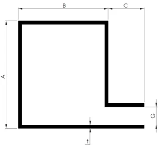
3.4 Cross section of the final geometry with dimensions illustrated. . . 52

3.5 Complete finite element model representing the structure along with

analytical rigid surfaces representing the fixture clamps and weld tips

(illustrated at the centre of the assembly). . . 55

3.6 Exploded view of the sheet metal components used to create the

assembly used in this study. . . 57

3.7 Laboratory Fixture used during the assembly process (a) during a

sub-assembly phase and (b) prior to final sub-assembly. . . 58

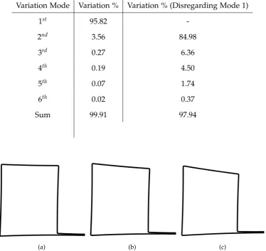
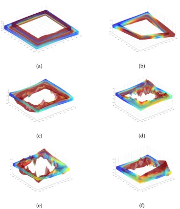
3.8 Gap variation modes extracted from scan measurement data: (a) Mode

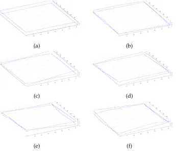
1, (b) Mode 2, (c) Mode 3, (d) Mode 4, (e) Mode 5 and (f) Mode 6. . . . 61

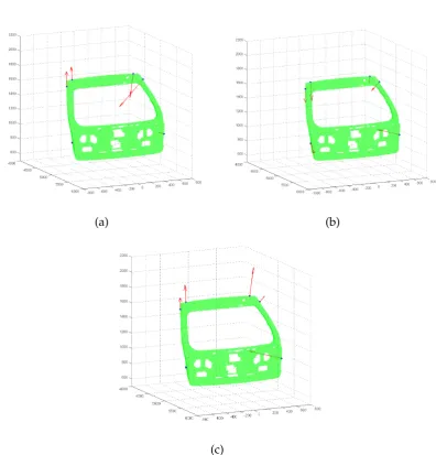
4.1 An exploded view of the sheet metal components that combine

together to create the closure assembly for a production sports utility

vehicle. . . 66

4.2 Production history data from standard measurements representing

mean shifts and variation in these measurements. Relative vector size

is indicative of magnitudes. . . 70

4.3 Dominant variation patterns observed in the six measurement points.

(a) Mode 1, (b) Mode 2, and (c) Mode 3. . . 72

4.4 Projected data points of the first three principal components of the

history data used with the KDE-PDM model applied to visualise the

distribution of these points. . . 74

4.5 Data point history mapped against variation pattern: (a) Mode 1, (b)

Mode 2 and (c) Mode 3. Series of graphs showing the apparent random

order of the sample components signifying there was no step shift in

(16)

5.1 Mapping of resulting twist for each joining sequence against the

spring-back twist. Twist scale provided as a measure of the principal

component and angular representation. Secondary y-axis detailing

the equivalent flushness difference from left to right caused by the

degree of structural twist. . . 84

5.2 Mapping of resulting twist for each joining sequence based on the gap

input deformation. Secondary y-axis detailing the equivalent flushness

difference from left to right caused by the degree of structural twist. . . 84

5.3 Cross section of deformed input gap variation at: (a) 2 mm, (b) 5 mm

and (c) 8 mm. This represents the primary variation mode in the

extracted data which is neglected for this study. . . 88

5.4 Extracted variation mode vectors across all simulated sequences and

gap variants: (a) Mode 1, (b) Mode 2, (c) Mode 3, (d) Mode 4, (e) Mode

5 and (f) Mode 6. . . 89

5.5 Mapping of the second principal component for the selected weld

sequences across all gaps. . . 90

5.6 Mean geometry from all simulations with colour-map illustrating

divergence from nominal. Illustrated as reference for the principal

component magnitudes. Ten times deformation shown. . . 91

5.7 Distributions for the selected curves based on the input distribution

with a mean of three millimeters and standard deviation of 0.5

millimeters. . . 91

5.8 Mapping of principal component 2the second principal component

(twist) for all weld sequences across all gaps. . . 92

5.9 Comparison of principal components 2 and 6 with the weld sequence

(17)

LIST OF FIGURES xvi

5.10 Plot of principal component coefficients for the second, third and

fourth components. Graph depicts the strong non-linear relationship

each individual sequence has between the patterns. A single line

representing a weld sequence, with the points representing the

simulated gap level. . . 94

5.11 Extracted variation mode vectors across all simulated weld and clamp

sequences, and gap variants: (a) Mode 1, (b) Mode 2, (c) Mode 3, (d)

Mode 4, (e) Mode 5 and (f) Mode 6. . . 96

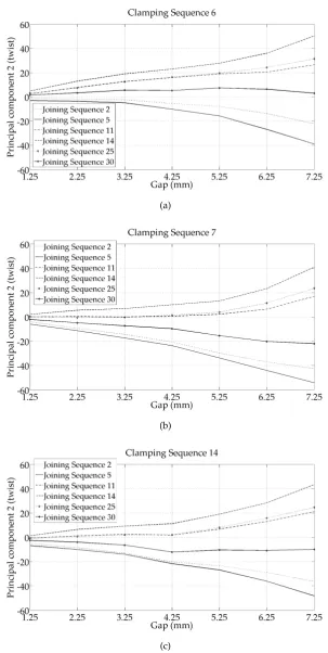
5.12 The second principal component mappings for each clamp sequence:

(a) Sequence 6, (b) Sequence 7, (c) Sequence 14, (d) Sequence 20, (e)

Sequence 21 and (f) Sequence 22. . . 97

5.12 The second principal component mappings for each clamp sequence:

(a) Sequence 6, (b) Sequence 7, (c) Sequence 14, (d) Sequence 20, (e)

Sequence 21 and (f) Sequence 22. . . 98

6.1 Analysis assumptions and relationships between joining sequence,

variability and structural design. . . 106

6.2 Two dimensional, two beam sequencing problem with exaggerated

example deformation. . . 107

6.3 Comparison of analysis by considering stress build-up and without

stress build-up. For variation pattern one, refer to Figure 6.8 (a). . . 108

stress build-up. For variation pattern two, refer to Figure 6.8 (b). . . 108

stress build-up. For variation pattern three, refer to Figure 6.8 (c). . . . 109

6.6 Comparison of final geometric positions by considering stress buildup

compared to without stress build-up for variation pattern three. . . 109

6.7 Example mapping of two different sequence curves given a particular

(18)

6.8 Variation patterns studied in the cantilever beam assembly

sequencing problem. (a) Variation pattern 1, (b) Variation pattern 2,

and (c) Variation pattern 3. . . 114

6.9 Mapping curve (a) and mapping curve derivative (b) for the first

variation pattern. . . 116

6.10 Mapping curve (a) and mapping curve derivative (b) for the second

6.11 Mapping curve (a) and mapping curve derivative (b) for the third

6.12 Two-dimensional, polygon-based beam assembly model with an

illustrative deformation applied. . . 120

6.13 Variation patterns for the polygon geometry (a) Pattern one, (b) Pattern

two, and (c) Pattern three. . . 121

6.14 Mapping and gradient curves for each input variation pattern

illustrating the selected sequences. (a) Pattern one (i) Mapping (ii)

Gradient, (b) Pattern two (i) Mapping (ii) Gradient, and (c) Pattern

three (i) Mapping (ii) Gradient. . . 123

three (i) Mapping (ii) Gradient. . . 124

(19)

LIST OF FIGURES xviii

6.15 Shape deformations for the weak-to-strong and fixed-to-free

methodologies modelled with and without internal stress build-up.

(a) Pattern one (i) Sequence 1-4-2-3 (ii) Sequence 3-2-4-1, (b) Pattern

two (i) Sequence 1-4-2-3 (ii) Sequence 3-2-4-1, and (c) Pattern three (i)

Sequence 1-4-2-3 (ii) Sequence 3-2-4-1. . . 126

6.16 Illustration of the increasing structural stress against the increase in

total variation of the polygon structure. . . 129

6.17 Comparison of robustness index against geometric profile change for

the polygon assembly. . . 130

6.18 Variation patterns for the nonagon geometry (a) Pattern one, and (b)

Pattern two. . . 132

6.19 Comparison of clamped and released geometries for two different

sequences: (a) Clamped configuration, (b) Released configuration. . . . 133

6.20 Preferred robust sequences for (a) the cantilever beam and (b) the

polygon geometries. . . 136

6.21 Cantilever beam sequence results presented by Liu and Hu (1995b). . . 137

7.1 Sequence calculated using the developed algorithm for the idealised

(20)

7.2 Simulated optimal joining sequence (Sequence 31) for (a) simultaneous

clamping configuration, and (b) clamping condition 1-2-3-4 (Clamp

sequence 21) configuration, presented against the poorest performing

simulated joining sequence (Sequence 14). . . 148

8.1 Set of laser-cut components. . . 154

8.2 Set of components bent into shape with joggle applied to the corner sections. . . 155

8.3 Set of upper components assembled with 16 joins. . . 156

8.4 Set of lower components assembled with 12 joins. . . 156

8.5 Example of outer lip to be joined during phase two of assembly. . . 157

8.6 Completed assembly with inner and outer connections made. . . 158

8.7 Positioning and mounting of Faro Co-ordinate measurement arm on assembly fixture. . . 159

8.8 Scanned measurement point cloud with point grid projected onto the surface for a top assembly. . . 160

8.9 Scanned measurement point cloud with point grid projected onto the surface for a bottom assembly. . . 160

8.10 Rotating bed and plate holding tooling elements with a physical stop used for limiting rotation to the same position. . . 161

8.11 Resistance spot welder mounted on rails with pin location system for positioning of joins on the assembly. . . 162

8.12 Illustration of brass limit blocks used to consistently position the resistance spot welder. . . 162

8.13 Clamping blocks holding the four components of the lower assembly in place where the corner joins are applied. . . 163

8.14 All components manufactured prior to the final assembly operation. . . 164

(21)

LIST OF FIGURES xx

8.16 Percentage reduction in the Root Mean Square (RMS) value of

variation for each sample group of five components at each gap level

for each sequence . . . 167

8.17 First variation mode of the two millimeter Principal Component

Analysis (PCA) analysis which is closest to representing the twist

variation mode. . . 168

8.18 First variation mode of the five millimeter PCA analysis which is

closest to representing the twist variation mode. . . 170

8.19 First variation mode of the five millimeter PCA analysis which is

closest to representing the twist variation mode. . . 171

8.20 Mapping of both the first and fourth principal component coefficient

illustrating groupings caused by different sequence selection. . . 172

8.21 Comparison of gap opening after joining. 8mm joined component with

plastic yielding at the weld zone, and (b) 2mm joined component with

no noticeable plastic yielding at the weld zone. . . 174

8.22 Overlay of prior simulation and digitised component geometry from

the experimental study. . . 175

8.23 Example of a distorted Finite element model generated utilising

scanned data. Colours illustrate deviation from intended design, with

red representing greatest and blue closest to nominal. . . 178

8.24 Experimental measurement points projected onto a simulated

geometry with 10x magnitude deformation. . . 178

8.25 Extracted variation modes across all revised simulated studies. (a)

Mode 1, (b) Mode 2, (c) Mode 3, (d) Mode 4, (e) Mode 5, (f) Mode 6,

(g) Mode 7 and (h) Mode 8. . . 180

8.26 Mapping of both the first and sixth principal component coefficient

illustrating the loss of relationship to sequence when new revised

(22)

8.27 Ability of a perfect rectangle to shear in comparison to a trapezoidal

geometry. (a) Initial rectangle, (b) Sheared rectangle, (c) Initial

irregular trapezoid, and (d) Sheared irregular trapezoid. . . 183

10.1 Illustrative example of the relationship between modelling complexity

and analysis accuracy placing this work in comparison to other works. 197

A.1 Procedure used to create the simulation input decks in the respective

simulation folder. . . 219

A.2 Procedural flow for the continuous execution of simulation on a given

quantity of processing cores. . . 220

A.3 Data extraction and processing procedure for the analysis of the

simulation database files. . . 221

B.1 Positions of each spot weld on the fixture. Illustration also indicated

the positions and numbering used in the simulated trials. . . 222

E.1 Mapping curve (a) and mapping curve derivative (b) for the first

variation mode used in the six join clamped polygon geometry. . . 229

E.2 Mapping curve (a) and mapping curve derivative (b) for the second

(23)

List of Tables

4.1 Process capability and process capability index across 30 of the

measurements. Numbered measurements begin at the top right

corner of the illustrations. . . 70

4.2 Variation modes, contributing variation percentage, per variation

pattern and cumulative variation. . . 73

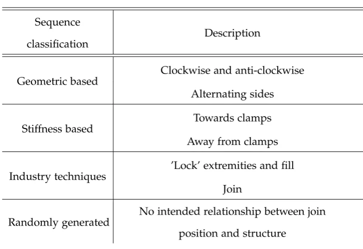
5.1 Tabulated descriptions of different joining sequence trends used in the

simulated study. . . 86

5.2 Individual principle component contributions for each weld sequence

and gap level. . . 87

5.3 Contribution of variation modes for 30 different weld sequences and 7

gap input variation levels. . . 88

5.4 Contribution of variation modes for six different weld sequences, six

different clamp sequences and seven gap input variation levels. . . 95

6.1 Summary of sequence analysis works for developing sequence

synthesis methodologies. . . 106

6.2 All two dimensional beam assembly problems simulated. . . 110

6.3 Robustness measure for selected sequences based on given input

variations for the cantilever geometry. The calculated robustness

measure indicated in brackets. . . 115

variations for the polygon geometry. . . 122

variations for the polygon geometry with clamping incorporated. . . 134

(24)

8.1 Complete experimental program with the selected sample numbers for

each gap size and the assigned sequence number. . . 165

8.2 Sequence and modal coefficient values for the twist principal

component in the two millimetre experimental data. . . 169

component in the five millimetre experimental data. . . 170

component in the five millimetre experimental data. . . 171

B.1 Access positions of spot weld gun for the relevant weld on the fixture. . 223

E.1 Sequence robustness evaluation for the cantilever geometry, ranked

according to their ability to reduce variation . . . 227

E.2 Sequence robustness evaluation for the polygon geometry, ranked

(25)

List of Acronyms

BIW Body In White

CAD Computer Aided Design

DCA Designated Component Analysis

DCT Discrete Cosine Transform

EAVS Elastic Assembly Variation Simulation

Efi Effective independence

FE Finite Element

FEA Finite Element Analysis

GD&T Geometric Dimensioning & Tolerancing

KDE-PDM Kernel Density Estimate - Point Distribution Model

MC Monte Carlo

MIC Method of Influence Coefficients

mm Millimetre

MPC Multi Point Constraint

PCA Principal Component Analysis

PCFR Place,Clamp,Fasten andRelease

PCMR Place,Clamp,Measure andRelease

(26)

PDM Point Distribution Model

RMS Root Mean Square

RSS Root Sum of Squares

RSW Resistive Spot Weld

SHS Square Hollow Section

SMA Statistical Modal Analysis

SOVA Stream of Variation Analysis

SQP Sequential Quadratic Programming

SUV Sports Utility Vehicle

(27)

Chapter1

Introduction

The quality of a product can be measured in a number of ways, the most important

being how it compares to the customer’s perceptions. Improving measures deemed

to be important to the aesthetics and functionality of a product will improve

customer perceptions of brand quality. This leads to increased sales and improved

brand reputation. This link is particularly evident in the automotive market, where

a reputation for poor quality vehicles can take decades to reverse and a brand’s

reputation for quality can take years to develop.

A customer’s perception of a high quality product is influenced by the product’s

ability to reliably perform to the customer’s expectations. As expectations increase,

a demand is placed on manufacturers to improve product quality. In the automotive

industry, some of the physical characteristics of a vehicle on which a customer builds

their perception of quality are: uneven gaps and flushness between panels, high

closure forces, and incorrect seal gaps leading to leaks and excessive vehicle interior

noise.

Improving product quality requires more detailed knowledge of the assembly

process and control of features critical to product functionality and aesthetic appeal.

As greater product quality is achieved, warranty costs will be reduced and customers’

perceptions of the brand’s quality will increase; leading to quicker production set up

due to decreased testing iterations and increased sales.

(28)

1.1 Background

The dimensional quality of a vehicle is the predominant factor affecting functionality

and aesthetics in the automotive market. Examples include: the flushness and gap

between panels; the sealing ability and general fit of closure assemblies; and the

effort required for opening and closing of these closure assemblies - all of which are

related to dimensional quality. Improving product quality therefore requires detailed

knowledge of the mechanics involved during assembly. Imperfections are inherent in

every manufactured part and when these imperfect parts are combined together to

create a more complex assembly, the dimensionality of the assembly will inherently

be a function of the individual components’ initial imperfections. Consequently, for

the assembly to function as intended, certain dimensional restrictions must be in

place not only on the assembly, but also on its constituents.

The relationship between a part and the final assembly dimensionality is the area

of tolerance design. Acceptable dimensional restrictions for the deviations of a part

from nominal are specified as tolerances; these allow manufacturers to work within

a range of the targeted dimension. Traditionally, the process of tolerance analysis is

applied to determine the final assembly level variation. This is often a cyclic process

where part design, manufacturing operation and tolerance specifications are revised

until the final assembly achieves its requirements - which can prove to be a costly

exercise. Alternatively, part tolerances can be estimated based on the desired final

assembly tolerance, a process know as tolerance synthesis or allocation.

Traditionally, the quality of assemblies is improved by increasing the accuracy

and precision of the individual components - a philosophy known as net build

(Hammett et al., 1998). Variations and deviations stack together, and the final

assembly dimensionality can be determined. However, all of the commonly applied

techniques (see Section 2.1) are based on the assumptions of rigid body assembly,

normal distributions and linearity. When analysing compliant bodies, such as sheet

(29)

§1.2 Problem Statement 3

these well known tolerance analysis models fail because they do not represent the

appropriate assembly mechanics.

1.2 Problem Statement

Sheet metal does not follow the traditional rigid body assembly laws, and to study

this, a variety of approaches have been developed to understand the mechanics of

assembly. Unfortunately, many of these are resource intensive or lack the ability to

adequately represent the assembly mechanics observed in certain situations. An

example of this is the degree of non-linearity present when studying clamp and

joining process sequencing. If this behaviour is not captured appropriately, then the

sequence appears to have either no influence or the results will be significantly

different in practice. When a detailed study investigating variational effects is

combined with sequence based assembly process design, it can often be unrealistic

to execute the large number of simulations or assembly trials required to adequately

understand the mechanics of that particular component’s assembly.

While to date focus has been been given to modelling the behaviour observed

during assembly, comparatively little attention has been given to the effect different

assembly joining sequences have on the assembly. Early work suggested that, as a

general rule, weld sequence should be performed from the weakest-to-strongest

area of the assembly (Liu and Hu, 1995b). However, other works suggested a

fixed-to-free end methodology; that would minimise internal stress buildup and, as

a consequence, was shown to reduce variation. Such statements are useful in a

production situation as they can enable more informed decisions to be made about

process sequencing. However, in some production situations these guideline, along

with other common industry practices, has not always been successful in reducing

variation - as presented by Wärmefjordet al.(2010c).

The impact on the final output variation is not only a function of the assembly

(30)

variations. Matuszyk et al. (2007) showed this for a slender top hat assembly

involving clamp sequencing. Furthermore, each shape variation was shown to

require a different ideal sequence, but it was possible to find a generic robust

solution. As mentioned, not all assembly guidelines have been successful in

minimising dimensional variation. This can be attributed to varying input

variations being undesirable with the sequences chosen, or the possibility that

certain variations cannot be controlled by joining sequence operations. This allows a

contrast to be made between the best sequence and the most robust sequence,

where the sequence the reduces variability the greatest for a particular input

variation, may perform poorly for another. Thus, a robust solution would be

preferable when no production variability information is available.

An understanding of the compliant assembly process is critical in developing

methods that seek to optimise the process. While researchers have focused on

developing models to represent the assembly process, to date comparatively little

focus has been given to understanding the generalised influence that different

operations have on compliant assemblies. Where studies have examined this, the

work has considered simplified lower dimensional situations that are not

representative of practical applications. Moreover, a unique possibility exists by

using the joining sequence to control variability because it can be freely altered in

existing production assemblies at minimal cost, even after vehicle launch. This work

addresses this opportunity using a combination of higher and lower dimensional

geometry cases to determine the requirements of joining sequence operations to

(31)

§1.3 Research question and objectives 5

1.3 Research question and objectives

1.3.1 Research question

As discussed in Sections 1.2 and 2.1.1, compliant bodies do not follow the

traditional rigid body assembly rules. Variations in the components propagate in a

non-linear manner as a consequence of geometric deformation and contact

conditions in manufacturing operations. As a result, there is an industry-wide need

for more detailed knowledge about the assembly of compliant bodies. This need is

addressed by the key research question of this work:

How can joining process sequencing be applied effectively to control

deformations and minimise dimensional variation during assembly of complex

non-ideal compliant components?

1.3.2 Objectives of this research

In addressing the aim, this work will focus on the analysis of different types of

incoming variability and the resulting impact on outgoing variability under realistic

processing conditions for use in practical applications. As such, it will centre on a

complex generalised assembly, rather than a specific case study or lower

dimensional representation. However, a case study will be utilised for topological

context, and a lower dimensional situation used to develop a deeper understanding

of the influencing factors in join sequencing. This research will address the aim by

focusing on the following four objectives:

Objective 1. Develop a geometry class to represent complex compliant assemblies.

The first component of this work simplifies an industrial case to develop an idealised

situation of the assembly process for further investigation. This involves interpreting

(32)

on a production situation. This objective addresses the area of the research question

relating to the complex non-ideal compliant assembly.

Objective 2. Demonstrate the interactions of process sequences and variations.

A significant component of this work is devoted to demonstrating the resulting

impact of the interactions between the incoming component variations, clamp

sequence, and joining process sequence on outgoing variation. To achieve this, the

simplified representative assembly from Objective 1 is used, and combined with

both computational simulation and experimental techniques for determining the

structure’s response. This forms the foundation of this thesis, and is used to answer

a number of sub-questions to the key research question, specifically:

1. When can weld sequence be used to control variation?

2. What is the impact of clamp sequencing on joining sequencing?

Objective 3. Determine the criteria for optimal sequence selection.

This objective involves determining the input conditions for an optimal joining

sequence. The assumptions used to model the analysis process are also considered

within the scope of this objective. A number of sequences can be defined as optimal;

however, for the purposes of this objective the three following research questions

are posed:

1. What is a robust sequence for minimising output variation given any input

dimensional variation pattern?

2. What is the influence of structural design on optimal sequence selection?

3. What is the significance of internal stress build-up to the analysis process?

Objective 4. Develop a method for the rapid identification of robust sequences.

(33)

§1.4 Structure of this thesis 7

robust sequence selection. This knowledge will be formalised in a procedural or

mathematical approach in order to develop an algorithm to determine a suitable

joining process sequence; henceforth allowing for faster setup and less guess work

where more complicated assemblies are concerned.

1.4 Structure of this thesis

To address the four objectives, this thesis is separated into seven proceeding chapters,

followed by the conclusions of this work. The structure is detailed in Figure 1.1.

Interpret process as observed in an industrial context and idealise

the geometrical situation for further analysis.

Create and validate a model of the assembly sequence process.

Investigate input variations and their interactions with process

variables.

Investigate a simplified model for sequence analysis, and

determine the requirements for optimal sequence selection.

Develop and demonstrate a sequence synthesis method for the

rapid identification of robust sequences.

Figure 1.1: The structure of this thesis, including the four objectives and the chapters in which they are addressed.

Firstly, a literature review is presented (Chapter 2) that provides an in-depth

(34)

compliant assembly and assembly in general. The methodology of this thesis then

follows (Chapter 3), which presents the methodological approaches used, and

includes the development of the idealised representative structure used throughout

the remainder of this work. This is then followed by an industrial context chapter

(Chapter 4), which aids in highlighting the applicability of the topology of the

structure developed in the methodology and specific limitations with existing

knowledge when confronted with a complex industrial application.

The next four chapters (Chapters 5, 6, 7 and 8) are devoted to the studies

performed on the idealised structure and the development of a generalised

algorithm. This can be separated into two areas: developing an understanding of

the process and its impact on variability; and developing an understanding of the

modelling assumptions and their impact on variability estimates for sequence

synthesis. Chapters 5 and 8 detail both computer-based simulations to study the

sequence dependence during assembly, and experimental-based trials for validation

of variation reduction through robust sequence selection. A study of the sequence

analysis process and modelling assumptions is provided in Chapter 6 by utilising a

simplified beam model with a variety of geometric forms. This is then followed by a

chapter that presents an algorithm for sequence synthesis (Chapter 7). Chapter 9

then presents a broader high level discussion on the application and place of this

work in the automotive and wider industries. The final chapter (Chapter 10)

presents the conclusions of this work and recommendations for future

(35)

Chapter2

Literature Review

This chapter presents a detailed review of the research involved in sheet metal

assembly, which, more broadly, is within the field of compliant body assembly. The

chapter begins with an overview of methods for tolerance analysis based on a rigid

body assumption (Section 2.1). Included here is an example application of possible

variation reduction observed in compliant assemblies to exemplify the shortcomings

of the discussed rigid body models. The next section (Section 2.2) presents a

detailed description of the assembly process and develops much of the terminology

used within this work. Specific attention is paid to common practices in industry.

This is then followed by a section on root cause diagnosis of variation (Section 2.3);

an area that formed the basis for much of the early research into sheet metal

assembly. Following this, a review of modelling techniques used to replicate the

assembly process is provided in Section 2.4. Since these models then form the basis

for studying variability within the assembly process, Section 2.5 reviews the

opportunities to minimise and control variability. Lastly, the chapter provides a

review of the work related to measurement and classification of variations and its

place within the design-to-manufacture process (Section 2.6). This highlights the

current issues and limitations of previously developed techniques to identify key

areas for investigation.

(36)

2.1 Background

The most common tolerance analysis techniques are the Worst Case (WC) and Root

Sum of Squares (RSS) (Chase and Parkinson, 1991). In the Worst Case model,

maximum variations are summed to produce the possible assembly variation. This

model guarantees assembly dimensional quality, but places tighter tolerances on the

part dimensions than are often required; therefore leading to an increase in

manufacturing costs. The RSS approach attempts to alleviate this issue by

considering a statistical model, where the part variations are assumed to be

normally distributed. The potential variation of two individual components of

length L1 and L2 when placed together can be estimated statistically, by applying

the law of propagation of uncertainties, expressed by Equation 2.1.

∆y=

v u u t n

∑

i=1

∂y ∂xi

2

∆xi2 (2.1)

Where the function y = f(x1,x2, . . . ,xn), in this case the function y can be

expressed as L=l1+l2representing the summation, or stacking of two components

of lengths l1 and l2. By applying the law of propagation of uncertainties the

variation inL can be expressed by Equation 2.2.

∆L=

q

∆l12+∆l22 (2.2)

This model allows for larger tolerance zones, which results in lower production

costs. However, it can also underestimate the required tolerance if skewness,

kurtosis, different input distributions, and/or mean shifts are present in the

measured data. Modified versions of the RSS model have been developed to take

into consideration some of these shortcomings and to allow for skewed inputs and

mean shifts. In higher dimensional situations, these techniques are based on vector

chains, either open or closed loop. These chains contain links that pass between the

(37)

§2.1 Background 11

final assembly variation.

2.1.1 Principals of compliant assembly

Takazawa’s (1980) research illustrated that flexible or compliant components, such

as sheet metal panels, do not follow the traditional rigid body assembly rules, and

that part variations could be absorbed through the assembly process. This ability to

absorb variations is based on a relationship between the joined and unjoined stiffness

of the parts.

The geometric stiffness is an important aspect in minimising dimensional

variability in compliant assemblies. The change in stiffness pre- to post- joining has

the ability to dictate the degree of spring-back when a deformed component is

released. This aspect of compliant assembly is not new; Hu and Koren (1997)

highlighted the relationship that exists between stiffness and variation during

multistage assembly. They showed that propagation of variation was closely

dependent on the type of assembly, either serial or parallel. For serial component

assembly, the resulting assembly became less rigid and consequently an increase in

variation was observed. For parallel assembly, such as closure assemblies, a

reduction in variation was observed due to the increase in stiffness of the whole. To

illustrate the relationship between structural stiffness and variability, an example of

a twisted component is provided(Figure 2.1).

(a) (b) (c)

Figure 2.1: Twisted component example, (a) before clamping, (b) after clamping and joining and (c) after final release. Colour scale highlighting the displacement from the nominal position.

(38)

position, joined and released. Here, a thin wall Square Hollow Section (SHS),

represented by Figure 2.1 is used. The section requires a moment applied to it for it

to lie flat. This moment can be determined based on elementary mechanics, where

the moment per unit angular deflection can be represented by Equation 2.3.

T

θ =

JG

L (2.3)

Here, J is the torsional moment of inertia, Gthe shear modulus andLthe length

of the beam. The process of joining the beams together along the open edge, alters

the torsional moment of inertia of the beam. Before joining, the torsional moment

of inertia for the beam can be calculated using Equation 2.4; by taking the sum of

the polar moment of inertia for each side of a square hollow section, as no shear

flow circuit exists over the beam’s cross section. After joining, the torsional moment

of inertia can be estimated by Equation 2.5, a known torsional property for SHS

members.

Jopen =Σ dt3

3 =

4(d−t)t3

3 (2.4)

JClosed =t(d−t)3 (2.5)

Where, for a rectangular section with equal sides, d is the width and height of

the rectangle and t is the material thickness. By determining the load applied to

the beam initially based on a level of deflection, then applying the opposite of this

load to the joined structure, the final assembly deformation can be determined using

Equation 2.6.

θout = 4 t2

(39)

§2.1 Background 13

By applying this to a 40mm SHS with a 1mm wall (Equation 2.7)

θout=8.77×10−4θin (2.7)

The variance of Equation 2.7 can then be determined by applying the law of

propagation of uncertainties presented in Equation 2.1. This results in the expected

variation presented in Equation 2.8.

σ_out2 = (8.77×10−4)2σ_in2 (2.8)

Given 10 degrees of twist variation prior to assembly, the equation can be completed

as shown in Equation 2.9.

σout=

q

(8.77×10−4₎2_×₁₀2 ₌_8.7_×₁₀−3_deg _(2.9)

As has been shown using the example of torsion in open and closed sections, by

joining the profile a significant increase in the geometric torsional stiffness occurs.

Since this increase causes a corresponding reduction in variation, it is this principle

that forms the basis for studying variation control in complex assemblies, such as

closure panels, where significant stiffness changes can occur.

2.1.2 Summary

The complete assembly process of compliant components, in this instance sheet

metal, can be considered as a step-based process involving incremental increases of

stiffness - such as the increase observed in the example. As each joining operation,

such as a spot weld or self piercing rivet, is performed, the compliant component is

pulled to a nominal location by the joining tool, then it is joined and released. When

released the component will return to a different location that will depend on the

stiffness of the components and the component geometry prior to the execution of

(40)

with each prior operation repeatedly clamping and releasing the assembly from and

to different locations. Additionally, each prior operation also results in internal

stresses in the components which may have an impact on the complete process,

particularly when the final assembly is released from the tooling elements (fixture)

used to locate the component for each of these sequenced joining operations. This

complete process is described in further detail in Section 2.2.

2.2 The Sheet Metal Assembly Process

The sheet metal assembly process is a complex series of operations that differs from

the traditional rigid body assembly processes. The compliant nature of the

components leads to assembly process interactions influencing the final assembly

output. These interactions make the assembly process difficult to model, sensitive to

process variables and problems, and make faults more difficult to diagnose. Given

these complexities, a wide variety of modelling and analysis approaches have been

used to understand the sheet metal assembly process. Previous research has applied

control theory, pattern recognition and artificial intelligence algorithms to

investigate these problems, and to attempt to reduce variations in production.

An automobile body, otherwise known as a Body In White (BIW), is constructed

from hundreds of individual components that are assembled together. To achieve the

end result, a large number of assembly operations are performed that build smaller

assemblies, or sub-assemblies, before they are combined to form larger assemblies,

and eventually the complete BIW. This process may be repeated many times, where

smaller sub-assemblies have other components added on; building on the assembly.

The most basic element of this larger chain of processes is a single assembly

process. Chang and Gossard (1997) represented the assembly of sheet metal

components by a four stage process, the Place, Clamp, Fasten andRelease (PCFR) cycle (Figure 2.2). Components are placed on an assembly station, aligned using

(41)

§2.2 The Sheet Metal Assembly Process 15

components onto the control surfaces. The fastening procedure is then performed;

this is commonly performed by spot welding, although self piercing rivets are also

used. Finally, the components are un-clamped from the assembly station.

Figure 2.2: The Place, Clamp, Fasten and Release cycle (Chang and Gossard, 1997)

To locate a component onto the assembly station, control strategies are used to

restrain the component’s available degrees of freedom. Translations and rotations

about each axis for a rigid component are restricted by a 3-2-1 locating system

(Figure 2.3). The locating strategy defines the number of points of contact in each

plane, where three points of contact are used in the primary datum plane, followed

by two in the secondary and one in the tertiary (Krulikowski, 2007). For compliant

bodies, Caiet al.(1996) showed that a N-2-1 locating strategy is effective in reducing

dimensional variability from external loading during the assembly of compliant

bodies. In this strategy, additional locating surfaces are used in the primary plane to

constrain the flexibility of the component and bring it to the desired position. The

secondary and tertiary planes are typically constrained using a locating pin with a

(42)

Figure 2.3: The 3-2-1 locating strategy. Clamps and pins are indicated byCi and Pi

respectively. In this example, the pins also coincide with the location of two of the locating surfaces. (Ceglarek and Shi, 1999)

The combination of control surfaces and pin tooling elements used to support a

workpiece are assembled into a supporting framework. These supporting

frameworks will be referred to as assembly fixtures. These assembly fixtures form

part of the assembly station, which also consists of the joining equipment and

appropriate safety equipment. The clamps that are used to hold the components

onto the control surfaces are most commonly pneumatically operated to aid the

automation of the assembly process.

The joining operation is then performed. The most common type of join is a

Resistive Spot Weld (RSW); however, self-piercing rivets are growing in use,

particularly when joining materials which are dissimilar or hard to join. For

resistive spot welding the methods of tip actuation and control can also vary. The

most common types are the positional and compensating tip control methods,

although servomechanism controlled tips are becoming increasingly popular. For

positional tip control, one weld tip is moved into position before the other is

clamped down onto it. Compensating weld tips close simultaneously and utilise

pneumatics as a force balance. Servomechanism controlled tips utilise force sensors

that can control the force exerted by the tips to control the position and clamping

force. The primary benefit of a servomechanism is the improved control of the force

(43)

§2.2 The Sheet Metal Assembly Process 17

2000).

Measurement of the assembly can be described by a similar technique, known

as the Place, Clamp, Measure andRelease (PCMR) (Ceglarek and Shi, 1999) cycle. In this cycle the components undergo a similar process, but are measured rather

than joined. In both the PCFR and PCMR process cycles, significant interactions and

deformations can occur to the component.

Due to the complexity of the sheet metal assembly process, any deviations of the

component from their target, or nominal, values become difficult to incorporate into

a tolerance analysis method. This affects the entire design-to-manufacture process,

and, as such, identifying the source of any variability within these deviations is

a critical concern. This can be visualised graphically by considering the potential

sources of variation using a fish-bone diagram, as shown in Figure 2.4. Due to the

need to understand the causes of variations in the assembly process, early work in

the area of sheet metal assembly focused on root cause diagnosis.

Figure 2.4: Fish-bone diagram illustrating potential root causes of variation that feed into the assembly process (Huet al., 2001)1

1_{Note that PCWR is used here to represent the PCFR cycle, where W refers to weld instead of F for}

(44)

2.3 Root cause diagnosis of variability

Determining the sources of variations is critical to quality improvement. Early work

showed that 72 percent of assembly variations in the sheet metal assembly process are

a result of faults in assembly fixtures (Ceglarek and Shi, 1995). To diagnose a fault,

a fault configuration is matched to an observed variation. In sheet metal assembly,

fault diagnosis is commonly considered as a simple linear mapping exercise; also

known as a parity relation (Venkatasubramanian et al., 2003), and is represented by

Equation 2.10.

x=D·v+ω (2.10)

Where x = [x1,x2, . . . ,xn]T is a random sample of n measurements; v =

[v1,v2, . . . ,vp]T is a vector representing the contribution of each fault; D= [d1,d2, . . . ,dp], is annx pconstant matrix, that represents the faults in the data;

andωis the uncorrelated noise. D, referred to as the diagnostic matrix is comprised

of a set of pdiagnostic vectors of length n. To diagnose faults, the diagnostic matrix

must first be determined. This can be achieved by using process information

(model-based) or through historical data (data-driven). Apley and Shi (2001)

presented a methodology that used factor analysis to estimate the diagnostic matrix

based on measurement data. Data-driven models have been proven to be useful to

identify variation sources (Apley and Lee, 2003); however, they suffer from pattern

interpretation in terms of the real physical process (Kong et al., 2008) and a lack of

historical data prevents their use in the early stages of production (Ronget al., 2000).

When a complete set of all faults is known, model-based pattern recognition

algorithms can be applied. Ceglarek and Shi (1996) used this approach in

identifying single fixture faults. Based on the fixture design, a set of diagnostic

vectors corresponding to each rigid body motion was formulated, as shown in

(45)

§2.3 Root cause diagnosis of variability 19

Figure 2.5: Fault manifestation of variation pattern for a 3-2-1 layout fixture (Ceglarek and Shi, 1999).

The measurement data were mapped onto the reduced data space generated by

performing Principal Component Analysis (PCA)2 on the diagnostic matrix. Fault matches were then determined using a minimum distance classifier. However, in

cases where excessive measurement noise is present, the fault is unknown or a new

variation pattern is observed from multiple faults, a misdiagnosis can be made.

Ceglarek and Shi (1999) presented an extension of this approach to incorporate

uncorrelated noise. Later, Ding et al. (2002) extended the application of PCA to

identify faults in a multi-stage process using a state-space model. This work

identified that it is not always possible to achieve complete diagnosis using PCA

due to the potential similarities between diagnostic vectors in multi-stage processes.

A more detailed pattern recognition algorithm, based on PCA, that is capable of

dealing with multiple faults, has also been proposed for a single station (Li and

Zhou, 2006) but has not been successfully translated to the multi-stage process.

Model-based methods that utilise direct estimation techniques allow for reduced

diagnostic sets to be used and predict faults using probability estimates. Ronget al.

(2000) combined diagnostic information obtained from the inverse stiffness matrix

of a beam model and PCA to identify the eigen-value/vector combinations from

measurement data. Hypothesis testing was then successfully applied to test the

plausibility of single faults given the diagnostic information. Kong et al. (2008)

presented a methodology for multiple fault diagnosis in a multi-station assembly

process by combining a state-space model with orthogonal diagonalisation analysis,

a method based on PCA. However, the variation patterns identified using PCA are

(46)

estimated as strictly orthogonal eigenvectors, whereas fixture faults can result in

non-orthogonal vectors. In addition, multiple variation patterns can be

compounded into one eigenvector representing maximum variation (Camelio and

Hu, 2004). As a result, PCA is capable of diagnosing a single fault but can be

insufficient for multiple fault diagnosis (Liu and Hu, 2005).

To address multiple fault diagnosis, Apley and Shi (1998) developed a method

using a least squares estimate. This approach was shown to be successful in

diagnosing multiple faults in an assembly fixture using a 3-2-1 locating strategy.

However, the ability for the technique to diagnose multiple faults depends on the

independence of the fault patterns. Noting this issue with the ability to diagnose,

Ronget al.(2001) developed an adjusted least squares approach which improved the

algorithm’s accuracy of diagnosis.

Liu and Hu (2005) presented another approach to address multiple fault

diagnosis when fault patterns may be close to co-linear. The technique uses

Designated Component Analysis (DCA), which has proved successful in diagnosing

multiple faults in both a 3-2-1 (Liu and Hu, 2005) and a N-2-1 (Camelio and Hu,

2004) locating strategy. The technique allows the fault pattern vectors to be selected

based on process knowledge. These designated patterns then need to form an

orthogonal set. Consequently, the set of patterns is then orthonormalised to convert

it to an orthogonal normalised basis (Lay, 2005). Unlike PCA, the components for

DCA do not need to be orthonormal and independent from the outset. For PCA an

orthogonal set is formed as a result of extracting the variation patterns. DCA has

proven more successful in diagnosing multiple fault patterns that are close to

co-linear than the least squares approach (Camelio and Hu, 2004). The approach

also allows greater physical significance of the patterns as they are dictateda priori.

DCA can be considered as a special case of the least squares algorithm where the

diagnostic vectors form an orthogonal set.

(47)

§2.3 Root cause diagnosis of variability 21

becomes significantly more difficult due to the potential co-linearity of the

diagnostic vectors. Ceglarek and Prakash (2011) developed the enhanced piecewise

least squares approach for diagnosis in these situations. The technique applies QR

factorisation3 _{as a method of orthonormalising the potentially ill-conditioned}

inverse stiffness matrix used as the diagnostic vectors, according to Stream of

Variation Analysis. The method proved successful in diagnosis for both a single and

a two fault case which were tested.

Previous research has also considered sensor placement for effective diagnosis of

faults. To determine the placement of the sensors, a complete diagnostic set of all

the fixture failures is required (Khan et al., 1999). Using a 3-2-1 locating strategy,

Khan et al. (1999) developed a constrained optimisation procedure in which the

objective was to maximise the distance between each dominant eigen-vector. A

diagnosability index was also developed to compare different sensor locating

positions and their ability to diagnose faults. The same technique was then

extended to locating sensors for single fault diagnosis in a multi-stage process

(Khan et al., 1998). Sensor positioning to identify multiple fixture faults in a N-2-1

locating strategy was studied by Camelio et al. (2005). The effective independence

method was applied to locate the sensors based on the diagnostic matrix assembled

from each single fixture fault. This method maximised the independence between

each of the sensors and showed the least squares estimate to be effective in

diagnosing multiple faults for the single assembly station.

Distributing sensor positions across the manufacturing process was also

considered by Khan and Ceglarek (2000) and was shown to improve the ability to

diagnose faults when compared to end of line measurements. More recently, Shukla

et al.(2013) developed an approach to distributed sensor placement with the specific

aim of feature based measurement across multiple stations. In this instance, the

features were key characteristics that were defined from Geometric Dimensioning &

Tolerancing (GD&T) information.