Multiple waves propagate in random particulate materials

White Rose Research Online URL for this paper:

http://eprints.whiterose.ac.uk/147112/

Version: Submitted Version

Article:

Gower, A.L. orcid.org/0000-0002-3229-5451, Parnell, W.J. and Abrahams, I.D. (Submitted:

2018) Multiple waves propagate in random particulate materials. arXiv. (Submitted)

© 2019 The Author(s). For reuse permissions, please contact the Author(s).

[email protected] https://eprints.whiterose.ac.uk/ Reuse

Items deposited in White Rose Research Online are protected by copyright, with all rights reserved unless indicated otherwise. They may be downloaded and/or printed for private study, or other acts as permitted by national copyright laws. The publisher or other rights holders may allow further reproduction and re-use of the full text version. This is indicated by the licence information on the White Rose Research Online record for the item.

Takedown

If you consider content in White Rose Research Online to be in breach of UK law, please notify us by

MATERIALS

ARTUR L. GOWER‡ †_{, WILLIAM J. PARNELL}‡_{, AND I. DAVID ABRAHAMS}§

Abstract. For over 70 years it has been assumed that scalar wave propagation in (ensemble-averaged) random particulate materials can be characterised by a single effective wavenumber. Here, however, we show that there exist many effective wavenumbers, each contributing to the effective transmitted wave field. Most of these contributions rapidly attenuate away from boundaries, but they make a significant contribution to the reflected and total transmitted field beyond the low-frequency regime. In some cases at leasttwo effective wavenumbers have the same order of attenuation. In these cases a single effective wavenumber does not accurately describe wave propagation even far away from boundaries. We develop an efficient method to calculate all of the contributions to the wave field for the scalar wave equation in two spatial dimensions, and then compare results with numerical finite-difference calculations. This new method is, to the authors’ knowledge, the first of its kind to give such accurate predictions across a broad frequency range and for general particle volume fractions.

Key words. wave propagation, random media, inhomogeneous media, composite materials, backscattering, multiple scattering, ensemble averaging

AMS subject classifications. 74J20, 45B05, 45E10, 82D30, 82D15, 78A48, 74A40

1. Introduction. Materials comprising small particles, inclusions or defects, randomly distributed inside an otherwise uniform host medium are ubiquitous. Com-monly occurring examples include composites, emulsions, dense suspensions, complex gases, polymers and foods. Understanding how electromagnetic, elastic, or acoustic waves propagate through such media is crucial to characterise these materials and also to design new materials that can control wave propagation. For example, we may wish to use wave techniques todetermine statistical information about the material, e.g. volume fraction of particles, particle radius distribution, etc.

The exact positions of all particles is usually unknown. The common approach to deal with this, which we adopt here, is to ensemble average over such unknowns. In certain scenarios, such as light scattering [38], it is easier to measure the average intensity of the wave, but these methods often need the ensemble-averaged field as a first step [14,54,53].

1.1. Historical perspective. The seminal work in this field is Foldy’s 1945 paper [14], which introduced the Foldy closure approximation in order to deduce a single ‘effective wavenumber’k∗in the formk∗=k0−φgwhereφis thevolume fraction of particles andg is the scattering coefficient associated with a single particle. Foldy introduced the notion of ensemble averaging the field, but the expression deduced for k∗ was restricted to dilute dispersions and isotropic scattering. Lax improved on this by incorporating a higher-order closure approximation [25, 26], now known as the ‘Quasi-Crystalline Approximation’ (QCA), and by including pair-correlation functions, which represent particle distributions. Both QCA and pair-correlations

∗_{Submitted to the editors October 2018.}

Funding: This work was funded EPSRC (EP/M026205/1,EP/L018039/1) and support from the Isaac Newton Institute (EP/K032208/1).

†_{Department of Mechanical Engineering, The University of Sheffield, UK ([email protected],} http://arturgower.github.io).

‡_{School of Mathematics, University of Manchester, Oxford Road, Manchester M13 9PL, UK.} § _{Isaac Newton Institute for Mathematical Sciences, 20 Clarkson Road, Cambridge CB3 0EH,}

UK

have now been extensively used in multiple scattering theory. The most commonly used pair-correlation is ’hole correction’ [13]. Both QCA and hole-correction are examples of statistical closure approximations [2,3], which are techniques widely used in statistical physics. For multiple scattering, the accuracy of these approximations has been supported by theoretical [33, 34], numerical [9] and experimental [59, 67] evidence. These approximations also make no explicit assumptions on the frequency range, material properties, or particle volume fraction. We note however that, to our are knowledge, there are no rigorous bounds for the error introduced by these approximations. For a brief discussion on these approximations see [21].

For an overview of the literature on multiple scattering in particulate materials, making use of closure approximations, see the books [55, 31, 38]. We now briefly summarise how calculating effective wavenumbers has evolved since the early work of Foldy and Lax.

Over the last 60 years, corrections to the dilute limit have been sought, mainly by expanding in the volume fractionφ and then attempting to determine the O(φ2₎ contribution to k∗. Twersky [56] obtained an expression for this contribution as a function off(π₋2θinc) andf(0), where θinc is the angle of incidence of an exciting plane wave, seeFigure 1, andf(θ) is the far field scattering pattern from one parti-cle [28]. The dependence on θinc implies that k∗ depends on the angle of incidence, which is counter-intuitive. Waterman & Truell [63] obtained the same expression as Twersky but with θinc = 0. However, [63] used a ‘slab pair-correlation function’ that (theoretically) limits the validity of their approach to dilute dispersions (small

φ), see [27] for comparisons with experiments and see [5] for a discussion in two di-mensions. Extensions that incorporate the hole-correction pair-correlation function were described by Fikioris & Waterman [13]. The Waterman & Truell expressions for three-dimensional (3D) elasticity are written down in [68, 45]. Work in 3D elastic-ity using QCA was reported by [8] andOther related work on effective wavenumbers, or more specifically effective attenutaion, on the low-frequency regime. Lloyd and Berry [30] calculated the O(φ2_{) contribution by including both QCA and hole} correc-tion for the scalar wave equacorrec-tion, although the language used stemmed from nuclear physics. More recently, [28, 29] re-derived the Lloyd & Berry formula for the effec-tive wavenumber without appealing to the so-called extinction theorem used in many previous papers, such as [60], and without recourse to ‘resumming series’. The work was then extended in order to calculate effective reflection and transmission in [32]. Gower et al. [21] subsequently extended this result to model multi-species materials, i.e. to account for polydisperse distributions.

Other related work on effective wavenumbers and attenuation include: comparing the properties of single realisations to that of effective waves [49,6,7,40], and effective waves in polycrystals [50, 64] such as steel and ceramics. The polycrystal papers use a similar framework to waves in particulate materials, except they assume weak scattering which excludes multiple scattering.

1.2. Overview of this paper. A commonassumption used across the field of random particulate materials, including those mentioned above, is to assume there ex-ists asingle, unique, complex effective wavenumber k∗that characterises the material. For example, for an incident wave eikx−iωt_{, of fixed frequencyω, exciting a half-space} (seeFigure 1) filled with particles, the tacit assumption is that the ensemble averaged wavehu(x)itravelling inside the particulate material takes the form

hu(x)_i=aeikx−iωt_+b

See [32] for a brief derivation. This assumption has been widely used in acous-tics [28,29, 31,12], elasticity [61,42, 43,46, 10] (including thermo-viscous effects), electromagnetism [58,59,52], and even quantum [51] waves. For example, it is a key step in deducing radiative transfer equations from first principles [35, 37].

In this work, we show however that theredoes not exist a single, unique effective wavenumber. Instead an infinite number of effective wavenumbersk1, k2, k3, ....exist, so that the average field inside the particulate material takes the form

hu(x)i=aeikx−iωt+ ∞

X

p=1

bpeikpx−iωt. (1.2)

In many scenarios, the majority of these waves are highly attenuating, i.e.kp has a large imaginary part forp >1. In these cases, the least attenuating wavenumberk1 will dominate the transmitted field in_hu(x)_i, andk1 will often be given by classical multiple scattering theory, as discussed in Subsection 1.1. However, these other ef-fective waves can still have a significant contribution to the reflected (backscattered) wave from a random particulate material, especially at higher frequencies and beyond the low volume fractionφlimit. Furthermore, there are scenarios where there are at least two effective wavenumbers, sayk1andk2, with the same order of attenuation. In these cases using only one effective wavenumber,k1 ork2, is insufficient to accurately calculate_hu(x)_i, even forxfar away from the interface between the homogeneous and particular materials.

We examine the simplest case that exhibits these multiple waves: two spatial dimensions (x, y) for the scalar wave equation, and consider particles placed in the half-space x > 0, which reflects incoming waves. We not only demonstrate that there are multiple effective wavenumbers, but we also use them to develop a highly accurate method to calculatehu(x)iand the reflection coefficient. This method agrees extremely well with numerical solutions, calculated using a finite difference method, but is more efficient. We provide software [17] that implements the methods presented and reproduce the results of this paper.

In a separate paper [18], we develop aproof that (1.2) is the analytical solution for the ensemble averaged wave. However, the proof in [18] is not constructive, in contrast to the work presented here, where we present a method that determines all effective waves (1.2).

We begin by deducing the governing equation for ensemble averaged waves in

Section 2. In Section 3we then show that multiple effective wavenumbers exist. To calculate these effective wavenumbers, we need to match them to the field near the interface at x= 0, which leads us to develop a discrete solution in Section 4. The discrete solution also serves as the basis for a numerical method, which we use later as a benchmark. InSection 5 we develop the Matching method, which incorporates all of the effective waves. InSection 6we summarise the fields and reflection coefficients calculated by the Matching method, the numerical method, and extant methods used in the literature. We subsequently compare their results inSection 7. InSection 8we summarise the main results of the paper and discuss future work.

2. Ensemble averaged multiple scattering. Consider a region Rfilled with

N particles or inclusions that are uniformly distributed. The field u is governed by the scalar wave equations:

∇2_u+k2_{u= 0, (in the background material),} (2.1)

∇2_u+k2

wherekandkoare the real wavenumbers of the background and inclusion materials, respectively. We assume all particles are the same, except for their position and rotation about their centre, for simplicity. For a distribution of particles, or multi-species, see [21].

In two dimensions, any incident wave∗ _v

j and scattered waveuj can be written in the form

vj(rj, θj) = ∞

X

n=−∞

vnjJn(krj)einθj, (2.3)

uj(rj, θj) = ∞

X

n=−∞

unjHn(krj)einθj, (2.4)

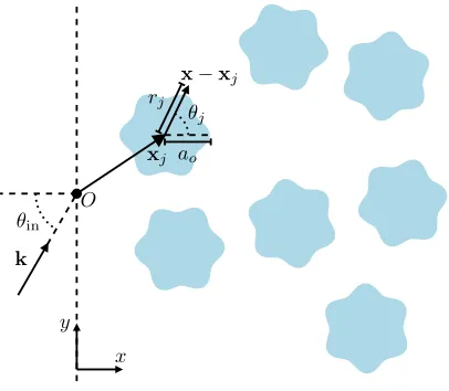
with (rj, θj) being the polar coordinates ofx−xj, andxj = (xj, yj) a vector pointing to the centre of thej-th particle, from some suitable origin, andxis any vector, see

Figure 1. The Jnand Hnare respectively Bessel and Hankel functions of the first kind. The representation (2.4) is valid whenrj is large enough for (rj, θj) to be outside of thej-th particle for allθj. For example, inFigure 1this distance would berj > ao.

ao θj x−xj rj

O xj

θin

k

y x

Fig. 1. Coordinates for particles with the origin O. The particles are only placed inx >0, that is, to the right of the dashed line. The vectork=k(cosθinc,sinθinc)shows the direction of the incident plane wave.

The T-matrix is a linear operator, in the form of an infinite matrix, such that

(2.5) unj= ∞

X

m=−∞

Tnm(τj)vmj for n=−∞, . . . ,∞ and j= 1, . . . , N ,

where we recall that N is the number of particles. The angleτj gives the particles rotation about their centre xj. Allowing particles to have different rotations, and assuming allτj∈[0,2π] to be equally likely, will lead to ensemble average equations that are equivalent to the equations for circular particles [39]. This matrixTexists

∗_{Equation (2.3) assumes that the incident wave originates outside of the of the j-th particle,}

when scattering is a linear operation (elastic scattering), and can accommodate par-ticles with a large variety of shapes and properties [15,16,62]; it is especially useful for multiple scattering [61,39,19].

The T-matrix also accounts for the particle’s boundary conditions. For instance, if u represents pressure, ρ and c are the background density and wave speed, the particles are circular with densityρo, sound-speedco, and radius ao, then continuity of pressure and displacement across the particle’s boundary [28, Section IV A], yields

(2.6) Tnm=−δnmZom, with Zom=

qoJm′ (kao)Jm(koao)−Jm(kao)Jm′ (koao)

qoHm′ (kao)Jm(koao)−Hm(kao)Jm′ (koao)

,

where qo = (ρoco)/(ρc) andko =ω/co. In this case the T-matrix is independent of the rotationτj.

In this paper we consider the incident plane wave

(2.7) uinc(x, y) = eik(xcosθinc+ysinθinc) for θinc∈(−π/2, π/2),

which excitesN particles, resulting in scattered waves of the form (2.4). SeeFigure 1

for an illustration. The total waveu, measured outside of all particles atx= (x, y), is the sum of all scattered waves plus the incident wave:

(2.8) u(x, y) =uinc(x, y) + N

X

j=1

uj(rj, θj).

To reach an equation for the coefficientsunj we write the total wave field incident on the j-th particle vj (2.3) as a combination of the incident wave plus the waves scattered by the other particles: vj(rj, θj) = uinc(x, y) +Pi6=jui(ri, θi). By then applying the Jacobi-Anger expansion touinc(x, y), using Graf’s addition theorem [31,

1], multiplying both sides byTqn, summing overn, and then using (2.5), we obtain

(2.9) uqj =uinc(xj, yj) ∞

X

n=−∞

Tqn(τj)ein(π/2−θinc)

+X

i6=j ∞

X

m,n=−∞

umiTqn(τj)Fm−n(kxi−kxj),

for all integersqandj= 1,2, . . . , N, where

(2.10) Fn(X) = (−1)neinΘHn(R),

and (R,Θ) are the polar coordinates ofX.

2.1. Ensemble averaging. In practice the exact position of the particles is unknown, so rather than determine the scattering from an exact configuration of particles, we ensemble average the field u over all possible particle rotations and positions in R. Sensing devices also naturally perform ensemble averaging due to their size or from time averaging [36]. See [14,45,21] for an introduction to ensemble-averaging of multiple scattering.

For simplicity, we assume the particle positions are independent of particle rota-tions, so that the probability of the particles being centred atx1,x2, . . . ,xN, is given by the probability density functionp(x1,x2, . . . ,xN). Hence, it follows that

(2.11)

Z

p(x1)dx1=

Z Z

where each integral is taken over_R. Further, we have

(2.12) p(x1, . . . ,xN) =p(xj)p(x1, . . . ,xN|xj),

wherep(x1, . . . ,xN|xj) is the conditional probability density of having particles cen-tred atx1, . . . ,xj, . . . ,xN (not includingxj), given that thej-th particle is centred at

xj. Given some functionF(x1, . . . ,xN), we denote itsensemble average(over particle positions) by

(2.13) _hF_i=

Z . . .

Z

F(x1, . . . ,xN)p(x1, . . . ,xN)dx1. . .dxN.

If we fix the location of the j-th particle, xj, and average over the positions of the other particles, we obtain aconditional averageofF given by

(2.14) hFixj =

Z . . .

Z

F(x1, . . . ,xN)p(x1, . . . ,xN|xj)dx1. . .dxj. . .dxN,

We assume that one particle is equally likely to be centred anywhere in_R, when the position of the other particles is unknown:

(2.15) p(xj) =

n

N, for xj ∈ R,

where we define the number densityn_{=N/|R|and the area of Ras |R|.}

Using the above we can expresshu(x, y)i, for (x, y) outside of the region R, by taking the ensemble average of both sides of (2.8) to obtain

hu(x, y)_i=uinc(x, y) + N

X

j=1

Z

Rh

uj(rj, θj)ixjp(xj)dxj (2.16)

=uinc(x, y) +n

Z

Rh

u1(r1, θ1)ix1dx1, for x6∈ R,

(2.17)

where we assumed that all particles are identical (apart from their position and ro-tation). We also used equations (2.12,2.15) and averaged both sides over particle rotations. Using the scattered field (2.4), we then reach

(2.18) hu1(r1, θ1)ix1 = ∞

X

n=−∞

hun1ix1Hn(kr1)e inθ1

.

The simplest scenario is the limit when the particles occupy the half-spacex1>0 [28], that is_R=_{(x, y)_|x >0_} . We focus on this case, although the method we present can be adapted to any region _R. In the limit of _R tending to a half-space, we let

N _{→ ∞}whilen_{remains fixed. Due to the symmetry between the incident wave (2.7)} and the half-space x1 >0, the field hun1ix1 has a translational symmetry along y1, which allows us to write [21]

(2.19) hun1ix1=An(kx1)e

iky1sinθinc

.

For step-by-step details on deriving a governing equation for An(kx1), see [28,

of equation (2.9), setj= 1, ensemble average over all particle rotations† _{and particle}

positions in x > 0, then use the statistical assumptions hole correction‡ and the quasicrystalline approximation, to reach the system:

(2.20) ∞

X

n=−∞ n

Z

x2>0 kx1−x2k>a12

TmAn(kx2)eik(y2−y1) sinθincFn−m(kx2−kx1)dx2

−Am(kx1) + eikx1cosθincTmeim(π/2−θinc)= 0, for x1>0,

where Tmδmq = (2π)−1R 2π

0 Tmq(τ)dτ,δmq = 1 if m=q and 0 otherwise, anda12 is the minimum allowed distance between the centre of any two particles. That is,a12 is at least twice the radius for circular particles. For the case shown in Figure 1we could choosea12= 2ao. This minimum distancea12 guarantees that particles do not overlap.

When the T-matrix T is known, we can determine the field An from the sys-tem (2.20). The aim of this paper is to efficiently solve for An and in the process reveal thatAn is composed of a series of effective waves.

For the rest of the paper we employ the non-dimensional variables

X1=kx1, X2=kx2, Roγ=ka12, φ=πn

R2 o

k2 =πn

a2 12

γ2, (2.21)

whereRo is the particles’ non-dimensional maximum radius (inFigure 1Ro =kao),

γ ≥ 2 a chosen closeness constant, with γ = 2 implying that particles can touch, and φ is the particle volume fraction§_{. Using non-dimensional parameters helps to}

formulate robust numerical methods and to explore the parameter space.

3. Effective waves. An elegant way to approximate An is to assume it is a plane wave of the form [31]

(3.1) _An(X) = ine−inϕAneiXKcosϕ for X >X,¯

whereKis the non-dimensional effective wavenumber (kKis the dimensional effective wavenumber), with Im K _≥ 0 to be physically reasonable, the factor ine−inϕ _{is for} later convenience, and ¯X is a length-scale we will determine later. We also restrict the complex angleϕby imposing that−π/2<Reϕ < π/2 and using

(3.2) Ksinϕ= sinθinc,

which is due to the translational symmetry of equation (2.20) iny1, see [21, Equation (4.4)]. This relation is often called Snell’s law.

As the material has been homogenised, it is tempting to make assumptions that are valid for homogeneous materials, such as assuming that only one plane wave (3.1) is transmitted into the material. When the particles are very small in comparison to the wavelength, this is asymptotically correct [44], but in all other regimes this is not valid, especially close to the edge ¯X = 0, as we show below.

†_{Assuming that every particle is equally and independently likely to be rotated by any angleτ}

j, which makes the ensemble-averaged T-matrix diagonal [57,39].

‡_{The assumption hole correction is not appropriate for long and narrow particles. More generally,}

the method we present can be applied to any pair correlations that depend only on inter-particle distance.

§_{For non-circular particles,φis slightly larger than the actual particle volume fraction because}

By substituting the ansatz (3.1) into (2.20), using (2.21) (see section SM1 for details) and by restrictingX1>X¯+γRo, we obtain

∞

X

n=−∞

Mmn(K)An= 0, Mmn(K) =−R2oδmn+ 2φTmNn−m (K) 1₋K2 , (3.3)

2φ

∞

X

n=−∞ einθinc

Ane−inϕe

i(Kcosϕ−cosθinc) ¯X

Kcosϕ₋cosθinc

= iπR2ocosθinc+g( ¯X), (3.4)

g( ¯X) = 2φ

∞

X

n=−∞ einθinc

(₋i)n−1

Z X¯

0 A

n(X2)e−iX2cosθincdX2, (3.5)

where

(3.6) Nn(K) =γRo(Hn′(γRo)Jn(γKRo)−KHn(γRo)Jn′(γKRo)),

and (3.4) is often called the extinction theorem, though we will refer to it as the extinction equation.

Using (3.3) we can calculate Kby solving

(3.7) det(Mmn(K)) = 0,

then the standard approach to calculate An is to use (3.3)1 and (3.4) and take ¯

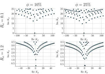
X = 0, which avoids the need to know An or to calculate g( ¯X). It is commonly assumed that there is only one viable K, when fixing all the material parameters, including the incident wavenumber k. However, in general (3.7) admits many solu-tions, which we denote asK=K1,K2,. . ., seeFigure 2for some examples. We order these wavenumbers so that Im Kp increases with p. There is no reason why these wavenumbers are not physically viable. Therefore we write_An as a sum of effective waves:

(3.8) _An(X) = in P

X

p=1

e−inϕp_Ap

neiXKpcosϕp for X >X,¯

where there are an infinite number of these effective wavenumbers [18], but to reach an approximate method we need only a finite numberP. Technically, (3.8) is a solution to (2.20) for X > 0, that is, we could take ¯X = 0. However, in this case, we found that close to X = 0 a very large number of effective waves P would be required to achieve an accurate solution. This is why we only use the sum of plane waves (3.8) forX >X >¯ 0.

One of these effective wavenumbers, in most cases the lowest attenuating K1, can be calculated using an asymptotic expansion for lowφ[28], and assuming it is a perturbation away from 1 (the background wavenumber).

Substituting (3.8) into (2.20) leads to the same dispersion equations (3.3) and (3.7), but withK1 andA1n replaced withKp andApn, which leads to

(3.9)

∞

X

n=−∞

Mmn(Kp)Apn = 0 and det(Mmn(Kp)) = 0,

while for the extinction equation (3.4) we need to substituteK forKp,ϕforϕp, and then sum overponly on the left-hand side to arrive at

2φ

P

X

p=1 ∞

X

n=−∞

Apnein(θ

inc−ϕp)e

i(Kpcosϕp−cosθinc) ¯X

Kpcosϕp−cosθinc

−100 ₋50 0 50 100 0

5 10 15 20 25

ReKp

Im

Kp

−100 −50 0 50 100 0

5 10 15 20 25

ReKp

Im

Kp

−40 −20 0 20 40 0.5

1.0 1.5 2.0 2.5 3.0 3.5

ReKp

Im

Kp

−40 −20 0 20 40 0.5

1.0 1.5 2.0 2.5 3.0 3.5

ReKp

Im

Kp

φ

= 10%

_φ

= 25%

R

=

0

.

1

R

=

1

.

2

Fig. 2.An example of the effective wavenumbersK1, K2, . . . that satisfy equation(3.9)2. The particles chosen are moderately strong scatterers, with T-matrix (2.6), parametersk= 1,ko= 2.0, co=ρo = 0.5,c=ρ= 1.0, and the non-dimensional radiusRo is0.2 for the top two graphs and 1.2for the bottom two graphs. Note that the bottom right graph shows two wavenumbers, almost on top of each other, both with imaginary part less than0.5.

for details see Section SM1. The question now arises: how do we calculate the un-knownsAp

n? Once each Kpandϕp are determined from (3.9)2and (3.2), then (3.9)1 can be used to write the vectorAp_{= [. . . , A}p

−n, A p

1−n, . . . , A p

n−1, Apn, . . .] in the form (3.11) Ap_=αp_ap _{and α= [α}1_{, α}2_{, . . .],}

where theap_{are determined from (3.9)}

1. However, only equation (3.10) remains to de-termine the vectorα. As there is more than one effective wave,P >1, equation (3.10) is not sufficient to determineα. This is because satisfying (3.9) and (3.10) only implies that the effective field (3.8) solves (2.20) forX1>X¯+γRo. The missing information, needed to determine α, will come from solving (2.20) for 0 _≤X1 <X¯ +γRo. We choose to do this by calculating a discrete solution for_An within 0≤X1<X¯+γRo, and then matching the An with the effective waves (3.8). The final result will be a (small) linear system (5.5).

4. A one-dimensional integral equation. Due to the symmetry between the halfspace and the incident wave, we can reduce (2.20) to a one-dimensional Wiener-Hopf integral equation:

(4.1) ∞

X

n=−∞

φ πR2

o

Z ∞

0

TmAn(X2)ψn−m(X2−X1)dX2

where

ψn(X) =Sn(X) +χ{|X|<Roγ}(Bn(X)−Sn(X)),

with χ{true} = 1 and χ{false} = 0, Sn(X) is given by (A.2) and Bn(X) is given by (A.6).

Gerhard [23] deduced a similar one-dimensional integral equation for electromag-netism, and in [18] we showed that the analytic solution to (4.1) is a sum of effective plane waves.

We will use (4.1) to determine the effective waves (3.8), and to formulate a com-pletely numerical solution to (2.20), which we use as a benchmark.

4.1. The discrete form. The simplest discrete solution of (4.1) is to use a regular spaced finite difference method and a finite-section approximation¶_{. A similar}

finite difference solution was used in [22]. Let_Aj

n=An(Xj) for Xj =jhandj= 0, . . . , J, with analogous notation for the other fields. We also define the vectors

A_{n = [A}0

n,A1n, . . . ,AJn], bn =−ein(π/2−θinc)Tn[eiX 0

cosθinc_{, . . . ,e}iXJcosθinc_]. (4.2)

For implementation purposes, we consider all vectors to be column vectors. We also use the block matrixA_{with components} A_n1=A_n, that is

(4.3) A_{= [. . . ,}A_−n,A_{1−n, . . . ,}A_n,A_{n+1, . . .],} soA_{can be viewed as a one column matrix. The goal is to solve for}A_.

To discretise the integrals in (4.1), we use R

f(X)dX ≈ P

jf(Xj)σj, which in the simplest form is σj = h for every j. Discretising the integrals in (4.1), then substituting (4.2), andX₁j=X₂j=jhforj= 0,1, . . . , J, leads to

(4.4) X

n (_Eℓ

nm+Rℓnm)−Aℓm+

X

n J

X

j=0

Qℓj

mnAjn=bℓm, for ℓ= 0,1, . . . , J,

whereq=_⌊Roγ/h⌋,

Qℓj mn=

φTm

πR2 o

σjSj−ℓn−m+

φTm

πR2 o

σℓj(Bn−mj−ℓ −Sn−mj−ℓ )χ{|j−ℓ|≤q}, (4.5)

Eℓ nm=

φTm

πR2 o

Z

X2≥XJ

An(X2)Sn−m(X2−Xℓ)dX2, (4.6)

Rℓ

nm=χ{ℓ>J−q}

φTm

πR2 o× (4.7)

Z Xℓ+Roγ

XJ A

n(X2)(Bn−m(X2−Xℓ, k)−Sn−m(X2−Xℓ))dX2.

Theσℓj depend on ℓbecause the discrete domain of integration |j−ℓ| ≤q changes withℓ, though the simplest choice would still be σℓj =h.

If we did not include _Eℓ

nm and Rℓnm, then the solution of (4.4) would represent the average wave in the layer 0_≤X_≤XJ_{. One method to calculate the solution for} the whole half-spaceX _≥0 is to extendXJ _until

An(XJ) tends to zero. However, it is more computationally efficient to calculate_Eℓ

nmandRℓnmby approximatingAn(X) as a sum of plane waves, as shown below.

¶_{The kernel in (2.20) does not satisfy the technical requirements in [11], and we have been unable}

5. Matching the discrete form and effective waves. Here we formulate a system to solve for the unknown effective wave amplitudesαp _{(3.11) andA(4.3). To} do this, we substitute_An(X2) for the effective waves (3.8) inEnmℓ andRℓnm(4.6,4.7), and we calculate the integralg( ¯X) in (3.10) by substituting_An(X2) for the discrete solution_Aj

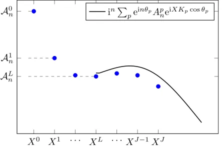
n(4.2). Finally, to determine theαp, and therefore the effective waves (3.8), we impose that (3.8) matches the discrete solution (4.2) in a thin layer near the boundary ¯X, for an illustration seeFigure 3. Imposing this match acts like a boundary condition for the effective waves. From here onwards we assume that ¯X =XL_.

X0 _X1 . . . XL . . . XJ−1_XJ A0

n

A1 n AL n

inP

peinθpApneiXKpcosθp

Fig. 3. An illustration of the discrete solution Ajn (4.2) (blue circles) and the effective waves (3.8)(black line). We restrict the coefficientsApnof the effective waves by imposing that the black line passes close to theAjn(i.e. satisfying the matching condiiton(5.10)) forX=XL, . . . , XJ, where we choseX¯ =XL_{. Increasing the number of effective waves will lead to a closer match} be-tween the discrete solution and effective waves.

5.1. Using the effective waves to calculate (4.6,4.7). Substituting the ef-fective waves (3.8) into (4.6), then integrating and using (A.2) we arrive at

(5.1) _Enmℓ = =

φTm

πR2 o

in+1Sn−mJ−ℓ P

X

p=1 eiXJ_K

pcosϕp_e−inϕp

Kpcosϕp+ cosθinc

Apn,

where we usedXJ

−Xℓ_=XJ−ℓ

≥0, forJ _≥ℓ, when substitutingSn−m(XJ−Xℓ) with (A.2). Employing (3.11), we write (5.1) in matrix form

(5.2) X

n Eℓ

nm= (Emα)ℓ, (Em)ℓp=

φTm

πR2 o

X

n

in+1_SJ−ℓ n−m

eiXJ_K

pcosϕp_e−inϕp

Kpcosϕp+ cosθinc

ap n.

To calculate (4.7), we first discretise the integral then substitute the effective waves (3.8), leading to

(5.3) Rℓ

nm=χ{ℓ>J−q}

φTm

πR2 o

ℓ+q

X

j=J

An(Xj)(Bn−mj−ℓ −S j−ℓ n−m)σℓj

=χ{ℓ>J−q}

φTmin

πR2 o

ℓ+q

X

j=J P

X

p=1

Apne−inϕpeiX

j_K

pcosϕp_(Bj−ℓ

where σℓj represents the discrete integral in the domain [XJ, Xℓ+q]. Using (3.11), just as we did in (5.2), we can write the above in a matrix form

(5.4) X

n

Rℓnm= (Rmα)ℓ.

We can now rewrite the integral equation (4.4), using the above equations, in the compact form

(5.5) (Em+Rm)α−IAm+

X

n

Q_mnA_n=bm,

which is valid for allm. Ifαwas known, then we could calculate the discrete solution A_{n from the above. However, the}α also depends on theA_{n, as we show below.}

5.2. The effective waves in terms of the discrete form. The equations to determine the effective waves, so far, are (3.9) and (3.10). To calculate the integral in (3.10), we discretise and substitute (4.2), which leads to the discrete form of the extinction equation (3.10):

(5.6) wTα=GTA_{+ iπR}2

ocosθinc,

where·T _{denotes the transpose, we used (4.3),g( ¯X) =G}T_A=P

nGTnAn,

wp= 2φ

∞

X

n=−∞ einθinc

e−inϕpe

i(Kpcosϕp−cosθinc)XL

Kpcosϕp−cosθinc

apn, (5.7)

(Gn)j= 2φeinθinc(−i)n−1e−iX

j_cosθ inc_σ

j, (5.8)

and as the domain of the integral in (3.10) is only up to XL _{= ¯X ≤ X}J_{, we set} (Gn)j = 0 forj > L.

When using P effective wavenumbers, there are P unknowns α1, . . . , αP, with, so far, only one scalar equation (5.6) to determine them. To determine the αp_{, we} match the sum of effective waves (3.8) with the discrete form _Aj

n in the interval:

XL_{< X < X}J_{, such as shown inFigure 3. To do this we could enforce}

(5.9) _Aj n = in

X

p

e−inϕp_eiXjKpcosϕp_ap

nαp=αTvjn, for j=L, L+ 1, . . . , J.

However, forn6= 0 the coefficientsAj

n andapncan be very small, and the above would not enforce the extinction equation (5.6). So rather than use (5.9) for every n, it is more robust to minimise the difference:

(5.10) 1

J−Lminα

X

n J

X

j=L |Aj

n−αTvjn|2 subject to wTα=GTA+ iπR2ocosθinc,

where the constraint enforces (5.6). For details on how to solve (5.10) seeSection SM2. The solution to the above is

(5.11) α=LTA₊iπR

2 ocosθinc

where w is the conjugate of w, the block matrix L _{= [. . . ,L−n,L1−n, . . . ,Ln, . . .],} with

LTA₌X

n

LTnAn, LTn =ZTn+w−1V−1w(GTn−wTZTn), (5.12)

V=X n

J

X

j=L

vj

n(vjn)T, ZTn = [0· · ·0 V−1vLn· · ·V−1vJn]. (5.13)

Finally, substitutingα(5.11) into (5.5) we reach an equation which we can solve forA_:

(5.14) ((E₊R₎LT₊M₎A₌B_{, (Matching method)}

whereE_andR_{have componentsEmandRm, given by (5.2) and (5.4), respectively,} while the components of block matricesB_andM_are

Bm=bm− iπR2

ocosθinc

wT_V−1_w (Em+Rm)V −1_w, (5.15)

Mmn=−δmnI+Qmn. (5.16)

To summarise, the terms w, V, and L _{are defined in the section immediately} above, Qmn is given by (4.5), and both A and bm are given by (4.2). The angle

θinc is the angle of the incident plane wave (2.7), Ro is a non-dimensional particle radius (2.21) which increases with the frequency. The block matricesG_, B_, A_,E_, R_, L_{, and}Z_{all have only one column. The elements of these columns are either column} vectors (Gm, Bm,Am) or matrices (Em,Rm,Lm, andZm).

5.3. The matching algorithm. We can now understand how to truncate the effective wave series (3.8): assume the wavenumbers Kp are ordered so that Im Kp increases withp= 1, . . . , P. Then note that the larger Im (XJ_K

pcosϕp) the less the contribution this effective wave will make to the matching (5.10),w(5.6),Rℓ

nm (5.3) and_Eℓ

nm(5.2). That is, we can chooseP such that Im (XJKPcosϕP) is large enough so that this wave will not affect the solutionA_.

To aid reproducibility, we explain how to solve equation (5.14), and determineA_, by using an algorithm inSection SM3.

6. The resulting methods. Here we summarise the Matching method, and other methods for solving (4.1). To differentiate between results for the different methods we use the superscriptsM, D, andO. That is, we denote the field_An(X) as

AM

n (X) (Matching method), ADn(X) (Discrete method), (6.1)

AOn(X) (One-effective-wave method). (6.2)

For the Matching method, we solve (5.14) to obtain

(6.3) _AMn (X) =

(

Aj

n= (An)j X=Xj inPP

p=1e−inϕpeiXKpcosϕpapnαp X > XJ

(Matching method)

where theαp_{are given from (5.11),ϕ}

The one-effective-wave method is the typical method used in the literature. It consists in using only one effective wavenumberK1, that is equation (3.1) withp= 1. This one wavenumber K1 is often given explicitly in terms of either a low volume fraction or low frequency expansion. However, as we explore both moderate frequency and volume fractions, we will instead numerically solve forK1, the least attenuating wavenumber. To solve forK1andA1n we take ¯X = 0 and numerically solve (3.9) and (3.10) forP =p= 1. The Snell angleϕ1 is determined from (3.2), withK=K1and

ϕ=ϕ1. The result is

(6.4) _AOn(X) = ine−inϕ 1

eiXK1cosϕ1

A1n (One-effective-wave method)

FromSubsection 4.1, we can devise a purely numerical method, which requires a much larger meshed domain forX. The resulting field is

(6.5) _ADn(Xj) =

(

(AD

n)j j≤J

0 j > J (Discrete method)

This discrete method gives a solution for a material occupying the layer 0< X < XJ andY _∈R_{. If the layer is deep enough, and the wave decays fast enough, then this} discrete method will be the solution for an infinite half-space. Algorithm SM3.1, in the supplementary material, can be used to calculate this discrete method by taking

P = 1,J =Linstead of step 7, as there is no matching region, and replace steps 9-15 with: solve forA_{by using}MAD_{=Binstead of (5.14).}

6.1. Reflection coefficient. The reflection coefficientR_{is the key information} required for many measurement techniques. We can compare the different methods for calculating the average wave by comparing their resulting reflection coefficient, which is much simpler than comparing the resulting fields_An(X).

Consider a particulate material occupying the region x > 0 and choose a point (x, y) to measure the reflection, with x < 0, then the ensemble average reflection coefficientR_{is such that}

(6.6) _hu(x, y)_i=uinc(x, y) +Reik(−xcosθinc+ysinθinc).

By combining (2.17-2.19), we conclude that

(6.7) R₌ φ

πR2 o

eiXcosθincX n

Z ∞

0 A

n(X1)

Z ∞

−∞

eiY0sinθinc

Fn(X0)dY0dX1,

where we usedX0=X1−Xand the non-dimensional parameters (2.21). The integral inY0 is given by (A.2) which, noting thatX0>0, leads to

(6.8) R₌ 2φ

πR2 ocosθinc

X

n

ine−inθinc

Z ∞

0 A

n(X1)eiX1cosθincdX1.

Substituting the Matching method field (6.3) into (6.8) leads to

(6.9)

RM ₌

∞

X

n=−∞

2φ πR2

ocosθinc ×

(Matching method)



i

n J

X

j=0

σjAjneiX

j_cosθ

inc−inθinc + i

P

X

p=1

αpapneinϕ

p refe

iXJ_(K

pcosϕp+cosθinc)

Kpcosϕp+ cosθinc



whereϕp_ref=π₋θinc−ϕp. For an interpretation of the reflection angleϕpref, see [21, Figure 7].

For the discrete method, we discretise (6.8), which leads to

(6.10) RD₌ ∞

X

n=−∞

2φ πR2

ocosθinc in

J

X

j=0

σjAjneiX

j_cosθ

inc−inθinc _{(Discrete method)}

Alternatively, to obtain the reflection coefficient for one effective wave (6.4), we set

J = 0 andP = 1 in (6.9) to reach

(6.11) RO₌ ∞

X

n=−∞

2φ πR2

ocosθinc

iA1 neinϕ

1 ref

K1cosϕ1+ cosθinc

(One-effective-wave method)

which agrees with equations (41) and (42) from [32], when expanding for low volume fractionφ.

7. Numerical experiments. For simplicity, we consider circular particles (2.6) for all numerical experiments, in which case, the non-dimensional radius (2.21)Ro=

aok, whereao is the particle radius.

For the material properties we use a background material filled with particles which either strongly or weakly scatter the incident wave given, respectively, by

co

c = 0.5, ρo

ρ = 0.5, (strong scatterers)

(7.1)

co

c = 1.1, ρo

ρ = 8.0, (weak scatterers)

(7.2)

noting thatρo ≫ρleads to weaker scattering thanρo ≪ρ. We will use a range of angles of incidence θinc, particle volume fractionsφ, and particle radiusesRo, which is equivalent to varying the incident wavenumbersk.

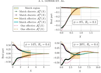
7.1. Comparing the fields. Figure 4shows several examples of_AM

n from (6.3). As a comparison we have shown the one-effective-wave fieldAO

n (6.4) as well. To not clutter the figure, we have not shown the discrete field AD

n (6.5), which would lie exactly on top of AM

n . Figure 4reveals how the discrete and effective wave parts of AM

n very closely overlap in the matching regionXL ≤X ≤XJ. This close overlap is not due to over-fitting, as there are more than double the number of equations than unknowns.

We now look closely at a specific case: particle volume fraction φ = 20% and non-dimensional particle radius Ro = 0.4 for the strong scatterers (7.1). Figure 5 shows the effective wavenumbers used and how the greater the attenuation Im Kp, the lower the resulting amplitude_|αP

|of the effective wave, and therefore the less it contributes to the total transmitted wave. We also see inFigure 5chow increasing the number of effective waves (while fixing everything else), results in a smaller difference between the fields of the matching and discrete methods. This clearly confirms that the field _An is composed of these multiple effective waves. Figure 6 shows how the Matching method (6.3) and the discrete method (6.5) closely overlap with

max X,n kA

M

n (X)− ADn(X)k= 4.5×10−4,

which is similar to the matching error 4.7_×10−5_{, given by the sum (5.10)}

0.0 0.5 1.0 1.5

−0.5

−0.4

−0.3

−0.2

−0.1 0.0

X

R

eal

p

ar

t

Match region Match discreteAM

0 (X) Match discreteAM

1 (X) Match effectiveAM

0 (X) Match effectiveAM

1 (X) One effectiveAO

0(X) One effectiveAO

1(X)

0 2 4 6 8

−0.50

−0.25

0.00 0.25 0.50

X

R

eal

p

ar

t

0.0 2.5 5.0 7.5 10.0

−0.50

−0.25

0.00 0.25 0.50

X

φ= 8%,Ro= 0.1

φ= 14%,Ro= 0.4 φ= 20%,Ro= 0.4

Fig. 4. These graphs show the matching field (6.3)and the one-effective-wave field (6.4) for a material with circular particles, incident wave angle θinc = 0, and properties (7.1). The non-dimensional radiusRo=kaoand volume fractionφare shown on each graph. Note that the discrete and effective part of the matching fields overlap in the match region. The one-effective-wave field in general loses accuracy close to the interfaceX= 0, which is why it gives inaccurate predictions for the reflection coefficientRO _(6.11).

when using the effective wavenumbers that satisfy (3.9). This agreement between the matching and discrete methods is not isolated to specific material properties and frequencies; we have yet to find a case where the two methods do not show excellent agreementk_{. Further, when increasing the number of effective wavenumbers P, and}

lowering the tolerancetolinAlgorithm SM3.1, the two methods converge to the same solution, as indicated byFigure 5c. In this paper we will not explore this convergence in detail, but we will show that the two methods produce the same reflection coefficient for a large parameter range.

7.2. Comparing reflection coefficients. The reflection coefficientR_{is a} sim-ple way to compare the different methods inSection 6. Many scattering experiments aim to estimate R_{[67,66]. The accuracy of estimating}R _{is also directly related to} the accuracy of calculating the transmitted waves.

InFigure 7we compare the reflection coefficient for the discrete methodRD_(6.10), Matching method RM _{(6.9) and two methods that use only one effective} wavenum-ber (6.11): one effective RO _{uses a numerical solution forK1 (the wavenumber with} the smallest imaginary part), while thelow vol. frac RO _{uses a low-volume-fraction} expansion for the wavenumber [32].

InFigure 7awe compare the reflection coefficients for strong scatterers (7.1) when varying the particle radius Ro (or likewise varying the wavenumberk) with a fixed

k_{Naturally, when the truncation error of the discrete method is very large, we found that the}

−30 −20 −10 0 10 20 30 1 2 3 4 5 6 7 ReKp Im Kp

−30 −15 0 15 30 0.0

0.2 0.4 0.6

Effective speed Re(Kp/ω)

Am p li tu d e | α P| a) b)

3 10 20 30 40

0.000 0.003 0.006

number of waves

m

ax

er

ror

c)

Fig. 5. These graphs show the influence of the effective wavenumbers for the strong scatter-ers (7.1) with particle volume fractionφ= 20%, non-dimensional radiusRo = 0.4, and incident wave angle θinc = 0.4. The resulting field AM_n is shown in Figures (6). a) shows the effective wavenumbers, with each marker corresponding to one wavenumberKP and its colour is stronger the larger the amplitude of its wave fieldαP_{. Clearly the larger the attenuation ImK}

p, the lower the amplitudeαP_{.b)reveals how the amplitudeα}P _{decreases when the effective phase speed increases in} magnitude. c)shows how the maximum error between the fields of the matching and discrete meth-ods decrease when increasing the number of effective waves used by the Matching method. Note, if we had not included the three lowest attenuating wavenumbers, the maximum error would be larger than0.17.

0 1 2 3 4 5

−0.6 −0.4 −0.2 0.0 0.2 X R eal p ar t

DiscreteAD

0

DiscreteAD

1

MatchAM

0

MatchAM

1

Wrong matchAM

0

Wrong matchAM

1

Zero matchAM

0

Zero matchAM

1

φ= 20%,Ro= 0.4

Fig. 6.This graph shows that the Matching method(6.3)overlaps with the discrete method(6.5) (a purely numerical method). The effective wavenumbers used are shown in Figure 5, and the material properties are given by (7.1). The dashed and dotted curves also result from the Matching method, but use the wrong effective waves: the dotted curve, wrong matchAM

0 andAM1 , use the effective wavenumbers (3.9)multiplied by1.2. The zero-matching fields zeros all the effective wave amplitudesapn= 0andAMn(X) = 0forX >1.

volume fractionφ= 20%. We use at most 1600 points for the X mesh, and less than 100 points for the X mesh of the Matching method, and aim for a tolerance of 10−5 for the fields.

We clearly see that RD _and RM _{(6.9) overlap. For Ro > 0.03 the maximum} difference maxRo|R

M

0.25 0.50 0.75 1.00 0.0

0.5 1.0

Ro

|

R

|

MatchedRM DiscreteRD One effectiveRO Low vol. frac. RO

0.5 1.0 1.5 2.0 2.5 3.0 −0.03

−0.02 −0.01 0.00 0.01

Ro

Im

R

a)

b)

Fig. 7. The reflection coefficients from the methods inSection 6 as a function of the non-dimensional particle radiusRo: a)has strong scattering particles(7.1)withφ= 20%andθinc= 0.0 whileb)has weak scattering particles(7.2)withφ= 25%andθinc= 0.4. Note the one-effective-wave fields almost overlap in this case. The real part of the curves inb) are even closer together, with max

Ro

|Re(RO_−RM_{)|= 0.0026for the one effectiveR}O_.

accuracy of the low-volume-fraction expansion depends on the type of scatterers and frequency [44], and can diverge in the limitRo→0 [20].

Figure 7b compares the reflection coefficients for weak scatterers (7.2). We use at most 2200 points for theX mesh, and less than 100 points for theX mesh of the Matching method, and aim for a tolerance of 10−5_{for the fields.}

Again, as before, we do not showRD_{for values ofRowhere the numerical} trunca-tion error become large (relative to our tolerance). For this case of weak scatterers we see that the difference between the methods is less, though the reflection coefficient is also smaller with mean|RM_{|= 0.058. Still, the relative error of Im (}RM₋RO_)≈10%. The imaginary part of the reflection coefficient, and where it changes sign, can be key for characterising random microstructure [48]. The real part of the reflection coeffi-cients is not shown, as the relative errors for the real part are even smaller.

effective wavenumbers.

Although there is an analytic proof [18] that there exists a series of effective waves, which solve the equations (2.20), this current paper shows how to calculate these by using a Matching method (6.3). In our numerical experiments inSection 7, we show that the Matching method converges to a numerical solution (the discrete method) for a broad range of wavenumbersk(or equivalently the non-dimensional radiusRo), particle volume fractions, and two sets of material properties. For examples,Figure 6

compares the average fieldsAn(X), andFigure 7the reflection coefficientsR of the matching and discrete methods. The drawback of the discrete method (6.5) is that it is computationally intensive, especially for low wave attenuation, requiring a spatial mesh between 1600 to 2000 elements to reach the same tolerance as the Matching method which used only 100 elements.

For small incident wavenumbers k, the Matching method converges to a result which assumes there exists only one effective wave for both strong and weak scatter-ers. Qualitatively, the fields_An(X) from the one-effective-wave (6.4) and Matching method (6.3) agreed well when moving away from the material’s interface, for example seeFigure 4. However, as the fields are not the same near the interface, the resulting reflection coefficients can significantly differ, as shown inFigure 7.

8.1. The next steps. Here we comment on a few directions for future work. One important limit, that we did not investigate here, is the low-volume fraction limit:

φ _≪ 1. In numerical experiments, not reported here, we found that the Matching method converges to the one-effective-wave method in the limit for lowφ. It appears that asφdecreases the ImKp, forp >2, tends to +∞, implying that the boundary layer ¯X shrinks and makes all but K1 insignificant. This limit deserves a detailed analytic investigation in a separate paper.

The consequences of this work directly impacts upon effective wave methods used for acoustic, elastic, electromagnetic, and even quantum wave scattering. That said, many of these fields use vector wave equations and require the average intensity. So one challenge is to translate the results of this paper to vector wave equations and the average intensity. Note that for electromagnetic waves, much of the groundwork for the average fields has already been done [23,24].

The radiative transfer equations are one outcome of properly deducing the aver-aged intensity for waves in particulate materials. For example, for electromagnetic waves, radiative transfer equations have been deduced under assumptions such as weak scattering, sparse particle volume fractions, and one effective wavenumber K1 [37]. Within the confines of the assumptions used, radiative transfer methods (and mod-ifications) are leading to accurate predictions of the reflected intensity [41,65, 47]. We speculate that this work will eventually lead to accurate predictions for reflected intensity for a broad range of frequencies and particles properties.

wavenum-bersand theMatching met, as well as the finite difference method we present.

Appendix A. Wiener-Hopf kernel. Here we reduce (2.20) to the Wiener-Hopf equation (4.1). First we separate the double integral:

Z

x2>0 kx2−x1k>a12

An(kx2)ei(y2−y1)ksinθincFn−m(kx2−kx1)dx2=

1

k2

Z

x2>0

An(X2)

Z

Y2_>R2 oγ

2_−X2

eiYsinθinc

Fn−m(X)dYdX,

where we usedX=kx2−kx1 and the parameters (2.21). We can then rewrite

(A.1)

Z

Y2 >R2

oγ 2

−X2

eiYsinθinc

Fn−m(X)dY =

χ{|X|<Roγ}Bn−m(X) +χ{|X|>Roγ}Sn−m(X),

whereχ{true}= 1 andχ{false}= 0. From [32, Eq. (37)] we have (A.2)

Sn(X) =

Z ∞

−∞

eiYsinθinc

Fn(X)dY = 2 cosθinc

(

ine−inθinc_eiXcosθinc _X ≥0,

(₋i)n_einθinc_e−iXcosθinc _{X <0.}

TheBn−m(X) in (A.1) only need to be evaluated for a small portion of the domain ofX, and are given by

(A.3) Bn(X) =

Z ∞

−∞

χ{Y2 >R2

oγ 2

−X2

}eiYsinθincFn(X)dY

= 2(−1)n

Z ∞

√ R2

oγ 2

−X2

cos (Y sinθinc+nΘ)Hn(R)dY.

Because the integrand tends to zero slowly as Y increases, we use an asymptotic approximation to evaluate the integral, namely

cos (Y sinθinc+nΘ) = cos((nπ)/2 +Ysin(θinc)) +O(X/Y), (A.4)

Hn(R) =−(−1)3/4e−inπ/2

r

2

πY +O(X

3/2_/Y3/2_), (A.5)

to rewrite

(A.6) Bn(X) = 2(−1)n

Z Y1 √

R2 oγ

2 −X2

cos (Ysinθinc+nΘ)Hn(R)dY+

(1 + i)eiY1(1−sinθinc) √

πY1cos2θinc

(₋1)ne2iY1sinθinc₍₁

−sinθinc) + 1 + sinθinc+O(X/Y1),

then as X is bounded by _|X_| < Roγ, we can choose Y1 such that X/Y1 is below a prescribed tolerance.

Substituting (A.1,A.2,A.6) into (2.20) leads to the Wiener-Hopf integral equa-tion (4.1).

[1] M. Abramowitz, Handbook of Mathematical Functions, American Journal of Physics, 34 (1966), pp. 177–177,https://doi.org/10.1119/1.1972842.

[2] G. Adomian, The closure approximation in the hierarchy equations, Journal of Statistical Physics, 3 (1971), pp. 127–133,https://doi.org/10.1007/BF01019846.

[3] G. Adomian and K. Malakian,Closure approximation error in the mean solution of stochastic differential equations by the hierarchy method, Journal of Statistical Physics, 21 (1979), pp. 181–189,https://doi.org/10.1007/BF01008697.

[4] T. Arens, S. N. Chandler-Wilde, and K. O. Haseloh,Solvability and spectral properties of integral equations on the real line: II. L p - spaces and applications, The Journal of Integral Equations and Applications, 15 (2003), pp. 1–35.

[5] C. Aristgui and Y. C. Angel, Effective material properties for shear-horizontal acous-tic waves in fiber composites, Physical Review E, 75 (2007), https://doi.org/10.1103/ PhysRevE.75.056607.

[6] L. Bennetts and M. Peter,Spectral Analysis of Wave Propagation through Rows of Scatterers via Random Sampling and a Coherent Potential Approximation, SIAM Journal on Applied Mathematics, 73 (2013), pp. 1613–1633,https://doi.org/10.1137/120903439.

[7] L. G. Bennetts, M. A. Peter, and H. Chung,Absence of localisation in ocean wave interac-tions with a rough seabed in intermediate water depth, The Quarterly Journal of Mechanics and Applied Mathematics, 68 (2015), pp. 97–113,https://doi.org/10.1093/qjmam/hbu024. [8] S. K. Bose and A. K. Mal,Longitudinal shear waves in a fiber-reinforced composite,

Inter-national Journal of Solids and Structures, 9 (1973), pp. 1075–1085.

[9] M. Chekroun, L. Le Marrec, B. Lombard, and J. Piraux,Time-domain numerical simula-tions of multiple scattering to extract elastic effective wavenumbers, Waves in Random and Complex Media, 22 (2012), pp. 398–422,https://doi.org/10.1080/17455030.2012.704432. [10] J.-M. Conoir and A. N. Norris, Effective wavenumbers and reflection coefficients for an

elastic medium containing random configurations of cylindrical scatterers, Wave Motion, 47 (2010), pp. 183–197,https://doi.org/10.1016/j.wavemoti.2009.09.004.

[11] F. de Hoog and I. H. Sloan,The finite-section approximation for integral equations on the half-line, The Journal of the Australian Mathematical Society. Series B. Applied Mathe-matics, 28 (1987), p. 415,https://doi.org/10.1017/S0334270000005506.

[12] J. Dubois, C. Aristgui, O. Poncelet, and A. L. Shuvalov, Coherent acoustic response of a screen containing a random distribution of scatterers: Comparison between different approaches, Journal of Physics: Conference Series, 269 (2011), p. 012004,https://doi.org/ 10.1088/1742-6596/269/1/012004.

[13] J. G. Fikioris and P. C. Waterman,Multiple Scattering of Waves. II. “Hole Corrections” in the Scalar Case, Journal of Mathematical Physics, 5 (1964), pp. 1413–1420, https: //doi.org/10.1063/1.1704077.

[14] L. L. Foldy,The multiple scattering of waves. I. General theory of isotropic scattering by randomly distributed scatterers, Physical Review, 67 (1945), p. 107.

[15] M. Ganesh and S. C. Hawkins,A far-field based T-matrix method for two dimensional obstacle scattering, ANZIAM Journal, 51 (2010), pp. 215–230.

[16] M. Ganesh and S. C. Hawkins,Algorithm 975: TMATROMA T-Matrix Reduced Order Model Software, ACM Trans. Math. Softw., 44 (2017), pp. 9:1–9:18, https://doi.org/10.1145/ 3054945.

[17] A. L. Gower,EffectiveWaves.jl: A package to calculate ensemble averaged waves in heteroge-neous materials., https://github.com/arturgower/EffectiveWaves.jl/tree/v0.2.0 (accessed 2018-24-10).https://github.com/arturgower/EffectiveWaves.jl/tree/v0.2.0.

[18] A. L. Gower, I. D. Abrahams, and W. J. Parnell,A Proof that Multiple Waves Propagate in Ensemble-Averaged Particulate Materials, arXiv:1905.06996 [cond-mat, physics:physics], (2019). arXiv: 1905.06996.

[19] A. L. Gower and J. Deakin,MultipleScattering.jl: A julia library for simulating, processing and plotting multiple scattering or waves.,https://github.com/jondea/MultipleScattering. jl(accessed 2017-12-29). original-date: 2017-07-10T10:06:59Z.

[20] A. L. Gower, R. M. Gower, J. Deakin, W. J. Parnell, and I. D. Abrahams,Characterising particulate random media from near-surface backscattering: A machine learning approach to predict particle size and concentration, EPL (Europhysics Letters), 122 (2018), p. 54001. [21] A. L. Gower, M. J. A. Smith, W. J. Parnell, and I. D. Abrahams, Reflection from a multi-species material and its transmitted effective wavenumber, Proc. R. Soc. A, 474 (2018), p. 20170864,https://doi.org/10.1098/rspa.2017.0864.

org/10.1016/j.jqsrt.2016.08.018.

[23] G. Kristensson,Coherent scattering by a collection of randomly located obstacles An alter-native integral equation formulation, Journal of Quantitative Spectroscopy and Radiative Transfer, 164 (2015), pp. 97–108,https://doi.org/10.1016/j.jqsrt.2015.06.004.

[24] G. Kristensson,Evaluation of some integrals relevant to multiple scattering by randomly dis-tributed obstacles, Journal of Mathematical Analysis and Applications, 432 (2015), pp. 324– 337,https://doi.org/10.1016/j.jmaa.2015.06.047.

[25] M. Lax,Multiple Scattering of Waves, Reviews of Modern Physics, 23 (1951), pp. 287–310,

https://doi.org/10.1103/RevModPhys.23.287.

[26] M. Lax, Multiple Scattering of Waves. II. The Effective Field in Dense Systems, Physical Review, 85 (1952), pp. 621–629,https://doi.org/10.1103/PhysRev.85.621.

[27] C. Layman, N. S. Murthy, R.-B. Yang, and J. Wu, The interaction of ultrasound with particulate composites, The Journal of the Acoustical Society of America, 119 (2006), p. 1449,https://doi.org/10.1121/1.2161450.

[28] C. M. Linton and P. A. Martin, Multiple scattering by random configurations of circu-lar cylinders: Second-order corrections for the effective wavenumber, The Journal of the Acoustical Society of America, 117 (2005), p. 3413,https://doi.org/10.1121/1.1904270. [29] C. M. Linton and P. A. Martin, Multiple Scattering by Multiple Spheres: A New Proof

of the Lloyd–Berry Formula for the Effective Wavenumber, SIAM Journal on Applied Mathematics, 66 (2006), pp. 1649–1668,https://doi.org/10.1137/050636401.

[30] P. Lloyd and M. V. Berry,Wave propagation through an assembly of spheres: IV. Rela-tions between different multiple scattering theories, Proceedings of the Physical Society, 91 (1967), p. 678,https://doi.org/10.1088/0370-1328/91/3/321.

[31] P. A. Martin, Multiple Scattering: Interaction of Time-Harmonic Waves with N Obstacles, Cambridge University Press, Cambridge, 2006, https://doi.org/10.1017/ CBO9780511735110.

[32] P. A. Martin,Multiple scattering by random configurations of circular cylinders: Reflection, transmission, and effective interface conditions, The Journal of the Acoustical Society of America, 129 (2011), pp. 1685–1695,https://doi.org/10.1121/1.3546098.

[33] P. A. Martin and A. Maurel,Multiple scattering by random configurations of circular cylin-ders: Weak scattering without closure assumptions, Wave Motion, 45 (2008), pp. 865–880,

https://doi.org/10.1016/j.wavemoti.2008.03.004.

[34] P. A. Martin, A. Maurel, and W. J. Parnell,Estimating the dynamic effective mass density of random composites, The Journal of the Acoustical Society of America, 128 (2010), pp. 571–577,https://doi.org/10.1121/1.3458849.

[35] M. I. Mishchenko, Vector radiative transfer equation for arbitrarily shaped and arbitrarily oriented particles: a microphysical derivation from statistical electromagnetics, Applied Optics, 41 (2002), pp. 7114–7134,https://doi.org/10.1364/AO.41.007114.

[36] M. I. Mishchenko, Multiple scattering, radiative transfer, and weak localization in dis-crete random media: Unified microphysical approach, Reviews of Geophysics, 46 (2008), p. RG2003,https://doi.org/10.1029/2007RG000230.

[37] M. I. Mishchenko, J. M. Dlugach, M. A. Yurkin, L. Bi, B. Cairns, L. Liu, R. L. Panetta, L. D. Travis, P. Yang, and N. T. Zakharova,First-principles modeling of electromag-netic scattering by discrete and discretely heterogeneous random media, Physics Reports, 632 (2016), pp. 1–75,https://doi.org/10.1016/j.physrep.2016.04.002. arXiv: 1605.06452. [38] M. I. Mishchenko, L. D. Travis, and A. A. Lacis,Multiple Scattering of Light by Particles:

Radiative Transfer and Coherent Backscattering, Cambridge University Press, 2006. [39] M. I. Mishchenko, L. D. Travis, and D. W. Mackowski,T-matrix computations of light

scat-tering by nonspherical particles: A review, Journal of Quantitative Spectroscopy and Ra-diative Transfer, 55 (1996), pp. 535–575,https://doi.org/10.1016/0022-4073(96)00002-7. [40] F. Montiel, V. Squire, and L. Bennetts,Evolution of Directional Wave Spectra Through

Finite Regular and Randomly Perturbed Arrays of Scatterers, SIAM Journal on Applied Mathematics, 75 (2015), pp. 630–651,https://doi.org/10.1137/140973906.

[41] K. Muinonen, M. I. Mishchenko, J. M. Dlugach, E. Zubko, A. Penttil, and G. Videen, Coherent Backscattering Verified Numerically for a Finite Volume of Spherical Particles, The Astrophysical Journal, 760 (2012), p. 118,https://doi.org/10.1088/0004-637X/760/ 2/118.

[42] A. N. Norris, Scattering of elastic waves by spherical inclusions with applications to low frequency wave propagation in composites, International Journal of Engineering Science, 24 (1986), pp. 1271–1282,https://doi.org/10.1016/0020-7225(86)90056-X.

Acous-tical Society of America, 131 (2012), pp. 1113–1120.

[44] W. J. Parnell and I. D. Abrahams, Multiple point scattering to determine the effective wavenumber and effective material properties of an inhomogeneous slab, Waves in Ran-dom and Complex Media, 20 (2010), pp. 678–701,https://doi.org/10.1080/17455030.2010. 510858.

[45] W. J. Parnell, I. D. Abrahams, and P. R. Brazier-Smith,Effective Properties of a Com-posite Half-Space: Exploring the Relationship Between Homogenization and Multiple-Scattering Theories, The Quarterly Journal of Mechanics and Applied Mathematics, 63 (2010), pp. 145–175,https://doi.org/10.1093/qjmam/hbq002.

[46] V. J. Pinfield,Thermo-elastic multiple scattering in random dispersions of spherical scatter-ers, The Journal of the Acoustical Society of America, 136 (2014), pp. 3008–3017. [47] J. Przybilla, M. Korn, and U. Wegler,Radiative transfer of elastic waves versus finite

difference simulations in two-dimensional random media, Journal of Geophysical Research: Solid Earth, 111 (2006),https://doi.org/10.1029/2005JB003952.

[48] R. Roncen, Z. E. A. Fellah, F. Simon, E. Piot, M. Fellah, E. Ogam, and C. Depollier, Bayesian inference for the ultrasonic characterization of rigid porous materials using re-flected waves by the first interface, The Journal of the Acoustical Society of America, 144 (2018), pp. 210–221,https://doi.org/10.1121/1.5044423.

[49] S. Rupprecht, L. G. Bennetts, and M. A. Peter,On the calculation of wave attenuation along rough strings using individual and effective fields, Wave Motion, 85 (2019), pp. 57–66,

https://doi.org/10.1016/j.wavemoti.2018.10.007.

[50] G. Sha,Correlation of elastic wave attenuation and scattering with volumetric grain size dis-tribution for polycrystals of statistically equiaxed grains, Wave Motion, 83 (2018), pp. 102– 110,https://doi.org/10.1016/j.wavemoti.2018.08.012.

[51] P. Sheng,Introduction to Wave Scattering, Localization and Mesoscopic Phenomena, vol. 88, Springer Science & Business Media, Aug. 2006.

[52] V. P. Tishkovets, E. V. Petrova, and M. I. Mishchenko,Scattering of electromagnetic waves by ensembles of particles and discrete random media, Journal of Quantitative Spec-troscopy and Radiative Transfer, 112 (2011), pp. 2095–2127, https://doi.org/10.1016/j. jqsrt.2011.04.010.

[53] L. Tsang, C. T. Chen, A. T. C. Chang, J. Guo, and K. H. Ding, Dense media radia-tive transfer theory based on quasicrystalline approximation with applications to pas-sive microwave remote sensing of snow, Radio Science, 35 (2000), pp. 731–749, https: //doi.org/10.1029/1999RS002270.

[54] L. Tsang and A. Ishimaru,Radiative Wave Equations for Vector Electromagnetic Propagation in Dense Nontenuous Media, Journal of Electromagnetic Waves and Applications, 1 (1987), pp. 59–72,https://doi.org/10.1163/156939387X00090.

[55] L. Tsang, J. A. Kong, and K.-H. Ding,Scattering of Electromagnetic Waves: Theories and Applications, John Wiley & Sons, Apr. 2004. Google-Books-ID: AFFJwOv16WsC. [56] V. Twersky,On Scattering of Waves by Random Distributions. I. FreeSpace Scatterer

For-malism, Journal of Mathematical Physics, 3 (1962), pp. 700–715,https://doi.org/10.1063/ 1.1724272.

[57] V. K. Varadan,Scattering of elastic waves by randomly distributed and oriented scatterers, The Journal of the Acoustical Society of America, 65 (1979), pp. 655–657,https://doi.org/ 10.1121/1.382419.

[58] V. K. Varadan, V. N. Bringi, and V. V. Varadan,Coherent electromagnetic wave prop-agation through randomly distributed dielectric scatterers, Physical Review D, 19 (1979), pp. 2480–2489,https://doi.org/10.1103/PhysRevD.19.2480.

[59] V. K. Varadan, V. N. Bringi, V. V. Varadan, and A. Ishimaru,Multiple scattering theory for waves in discrete random media and comparison with experiments, Radio Science, 18 (1983), pp. 321–327,https://doi.org/10.1029/RS018i003p00321.

[60] V. K. Varadan, Y. Ma, and V. V. Varadan,A multiple scattering theory for elastic wave propagation in discrete random media, The Journal of the Acoustical Society of America, 77 (1985), pp. 375–385,https://doi.org/10.1121/1.391910.

[61] V. K. Varadan, V. V. Varadan, and Y.-H. Pao, Multiple scattering of elastic waves by cylinders of arbitrary cross section. I. SH waves, The Journal of the Acoustical Society of America, 63 (1978), pp. 1310–1319.

[62] P. C. Waterman,Symmetry, Unitarity, and Geometry in Electromagnetic Scattering, Physical Review D, 3 (1971), pp. 825–839,https://doi.org/10.1103/PhysRevD.3.825.

[63] P. C. Waterman and R. Truell,Multiple Scattering of Waves, Journal of Mathematical Physics, 2 (1961), p. 512,https://doi.org/10.1063/1.1703737.

of Solids, 38 (1990), pp. 55–86,https://doi.org/10.1016/0022-5096(90)90021-U.

[65] U. Wegler, M. Korn, and J. Przybilla,Modeling Full Seismogram Envelopes Using Radia-tive Transfer Theory with Born Scattering Coefficients, Pure and Applied Geophysics, 163 (2006), pp. 503–531,https://doi.org/10.1007/s00024-005-0027-5.

[66] R. Weser, S. Wckel, B. Wessely, and U. Hempel, Particle characterisation in highly concentrated dispersions using ultrasonic backscattering method, Ultrasonics, 53 (2013), pp. 706–716,https://doi.org/10.1016/j.ultras.2012.10.013.

[67] R. West, D. Gibbs, L. Tsang, and A. K. Fung,Comparison of optical scattering experiments and the quasi-crystalline approximation for dense media, Journal of the Optical Society of America A, 11 (1994), pp. 1854–1858,https://doi.org/10.1364/JOSAA.11.001854. [68] R.-B. Yang,A Dynamic Generalized Self-Consistent Model for Wave Propagation in