Modelling the Nonlinear Oscillations Due to Vertical Bouncing Using a Multi-Scale Restoring Force System Identification Method

This is a repository copy of Modelling the Nonlinear Oscillations Due to Vertical Bouncing

Using a Multi-Scale Restoring Force System Identification Method.

White Rose Research Online URL for this paper:

http://eprints.whiterose.ac.uk/129015/

Version: Accepted Version

Article:

Guo, Y., Guo, L., Racic, V. et al. (2 more authors) (2018) Modelling the Nonlinear

Oscillations Due to Vertical Bouncing Using a Multi-Scale Restoring Force System

Identification Method. International Journal of Signal and Imaging Systems Engineering.

ISSN 1748-0698

https://doi.org/10.1504/IJSISE.2018.10011744

[email protected] https://eprints.whiterose.ac.uk/ Reuse

Items deposited in White Rose Research Online are protected by copyright, with all rights reserved unless indicated otherwise. They may be downloaded and/or printed for private study, or other acts as permitted by national copyright laws. The publisher or other rights holders may allow further reproduction and re-use of the full text version. This is indicated by the licence information on the White Rose Research Online record for the item.

Takedown

If you consider content in White Rose Research Online to be in breach of UK law, please notify us by

1

Modelling the Nonlinear Oscillations Due to

Vertical Bouncing Using a Multi Scale

Restoring Force System Identification Method

Yuzhu Guo1,2,3_{, Lingzhong Guo}1,3_{, Vitomir Racic}3,4,5_{, Shu Wang}4_{, and S. A. Billings}1,3

1 _{Department of Automatic Control and Systems Engineering}

The University of Sheffield, Sheffield, UK

2 _{School of Automation Science and Electrical Engineering}

Beihang University, Beijing, China

3 _{INSIGNEO institute for in silico Medicine}

The University of Sheffield, Sheffield, UK

4 _{Department of Civil and Structural Engineering}

The University of Sheffield, Sheffield, UK

5_{Department of Civil and Environmental Engineering}

Politecnico di Milanok, Milan, Italy

Abstract

Human vertical bouncing motion is studied using a system identification method. A multi-scale

mathematical model is identified directly from real experimental data to characterise the nonlinear

oscillation associated with the vertical bouncing. A new method which combines the restoring force

surface method and the iterative orthogonal forward regression algorithm is proposed to determine

the model structure and estimate the associated parameters. Two types of sub-models are used to

study the nonlinear oscillations in different scales. Results show that the model predicted outputs

provide excellent predictions of the experimental data and the models are capable of reproducing the

nonlinear oscillations in both time and frequency domain.

Key words:

1. Introduction

Studies of the induced dynamic load that arises from people walking and bouncing is an important

subject in many fields including biomechanics, medical science, sports science, robotics, control

systems, and also civil engineering. Many authors have studied the motion of the human body in

walking, jumping, and bouncing from different aspects (Blickhan, 1989; Ernesto & Tianjian, 2009;

2 Vitomir Racic & Chen, 2015; V. Racic & Pavic, 2010a, 2010b; V. Racic, Pavic, & Brownjohn, 2009;

Spägele, Kistner, & Gollhofer, 1999a, 1999b; van Werkhoven & Piazza, 2013).

A complete representation of body motion introduced by bouncing includes the modelling of vertical,

lateral, and longitudinal motions (Garcia, 1999). The vertical component is often studied as part of the

crowd-structure interaction in civil engineering while the lateral and longitudinal components are

often studied for the lateral stability of the human body during walking and bouncing. In this paper,

only the vertical motion due to human bouncing will be investigated.

In this paper, the motion of a marked point on the chest of a test subject during bouncing is recorded

and investigated using a system identification method. The modelling of the motion of human body

can be very complicated because of the following difficulties. Firstly, the human body is composed of

several connected segments: head, trunk, arms, legs, feet and so on. These segments are connected

by joints and interact with each other in motion. Each of these segments may have a complex effect

on the motion of a specific point and the effect is unknown. For instance, the motion of the head

depends on the movements of trunk, legs, ankles, and so on. In the robotics, especially in the

investigation of the stability of robots, the motion of a robot is often simplified as a multi-link inverted

pendulum. The movement of the top-end could be very complex because of the effects from the lower

segments of the system. Another source of complexity is that the mass of the human body is neither

lumped in a mass centre nor distributed uniformly. Therefore, modelling the motion of the marked

point using a first principles method can be very difficult. In this paper a system identification method

is used to study the motion of a marked point of human body which is on a relatively high position of

the human body and the motion of this point is of rich dynamics. In the investigation of complex

systems, a system identification method often has significant advantages. The system to be identified

is considered as a black box, which avoids the complex underlying mechanism in the system. The data

of interest are collected through experimental methods and the relationships between these

observations are studied.

In this paper, a continuous time model will be identified for the body motion in vertical bouncing by

studying the relationships between the displacement, velocity and accelerations. This method is

known as the restoring force surface method (RFS). Restoring force surface method as an ideal method

for the study of nonlinear dynamics has been widely used since the first introduction (Masri, Bekey,

Sassi, & Caughey, 1982; Masri & Caughey, 1979). Restoring force surface method which converts the

problem of modelling nonlinear dynamics into the surface fitting in the state space significantly

simplified the modelling process. The restoring force surface is usually reconstructed using the

3 yields insight into the physical system. This allows one to qualitatively study the primary difficulties

encountered in nonlinear system identification: what nonlinearities involve in the system and how

these nonlinearities affect the dynamics behaviours of the system. For some more complex cases

where the restoring force surface cannot be represented using a uniform nonlinear function, a

piecewise models (Allen, Sumali, & Epp, 2008) and local restoring force surface method have been

studied (S. W. R. Duym, Schoukens, & Guillaume, 1996). For a complete discussion of the restoring

force surface method, readers are referred W T (Worden & Tomlinson,

2001) and the related papers (Worden, 1990a, 1990b). Some quantitative methods have also been

intensively studied especially the direct parameter estimation methods (Worden & Tomlinson, 2001).

However, the problems that which set of nonlinearities are involved in the system dynamics and how

to get a minimum set of nonlinearities which is sufficient to represent the systems seems not to be

perfectly answered.

In this paper, a new method which combines the restoring force surface method with the iterative

orthogonal forward regression (iOFR) algorithm (Yuzhu Guo, L.Z. Guo, S. A. Billings, & H. L. Wei, 2015c)

will be introduced to try to give a satisfying answer to these problems. The orthogonal forward

regression algorithm (is also known as forward orthogonal least squares regression algorithm) and the

associated error reduction ratio (ERR ) have been proved to be powerful tools for determination of

nonlinear model structures in various ranges of applications (S. A. Billings, 2013). The OFR algorithm

has recently been used to identify nonlinear continuous time models (Yuzhu Guo, Guo, Billings, & Lang,

2015; Yuzhu Guo, Guo, Billings, & Wei, 2016). The iOFR algorithm is an improvement to the classic OFR

algorithm. The iOFR has been proved to work better under a non-persistent excited condition (Yuzhu

Guo, L. Z. Guo, S. A. Billings, & H. L. Wei, 2015b). In the application of the orthogonal forward

regression algorithm, a very wide range of terms can be used according the needs of the practical

systems, such as, polynomials, rational functions, spline functions, radial basis functions (RBFs),

wavelet functions, and so on (Stephen A. Billings, Wei, & Balikhin, 2007; Wei, Zhu, Billings, & Balikhin,

2007). Because of the complexity of the system under consideration, three different types of

regressors will be used in this paper to model the body motion due to vertical bouncing: the

polynomials, multi-scale radial basis functions (or wavelets) and the hybrid regressors which combine

the first two kinds of functions.

The iterative orthogonal forward regression restoring force surface method is capable to model a

complex restoring force surface. For example the non-uniform restoring force surface can be

identified using piecewise spline functions or radial basis functions as regressors to obtain a parsimony

4 functions (S. A. Billings & Wei, 2005) will be combined with the restoring force surface method to give

a coarse to fine representation of the nonlinear oscillation in body motion.

Since the body motion in this study is the source of the human-introduced dynamic forces the study

of the nonlinear oscillation is of a significant meaning in study of the ground reaction force. The

introduce method can also be directly used to study the relations between the body motion and the

ground reaction forces by replacing the measured restoring force with the ground reaction force(Y.

Guo et al., 2017). The nonlinear oscillation of the marked point on body trunk instead of the ground

reaction force is studied because experimental data show that the motion of body trunk is of a richer

dynamics compared with the ground reaction force. A direct recovering of the ground reaction forces

using the same method will be studied in a separate paper.

This paper is organised as follows: Section 2 briefly explained the experiment from which data were

collected and the preliminary analysis of these data. Section 3 introduced the new iterative orthogonal

forward regression restoring force surface method. Three different kinds of sub-models are used to

identify the body motion in section 4. The advantages and disadvantages of each model are discussed.

The conclusions are finally drawn in section 5.

2. Experiment and data analysis

2.1 Experiment

The experiment was conducted in the Department of Civil and Structural Engineering, the University

of Sheffield, Sheffield, UK. This study has been approved by the Research Ethics Committee of the

University of Sheffield and conforms to the ethical guidelines.

A test subject bounced on an AMTI BP-400600 force plate following a 1.2 Hz metronome beat. The

body motion was measured using optical motion capture technology. Two markers were attached on

the chest and pelvis of the test subject, respectively. Cameras recorder the movements

(displacements, velocities and accelerations) of the target markers in real time. The test last 35s and

the recorded signals were sampled at 200Hz. Figure 1 shows the recorded displacement, velocity, and

the acceleration signals of the chest marker.

In this paper the vertical motion of the marker on chest is studied. This point is studied because this

point is at a relatively high position of the human body. The effects from the lower parts of human

5 same time, since this point was chosen on the line of symmetry of the body the influent from the

lateral movement is small and negligible.

Figure 1 Recorded signals

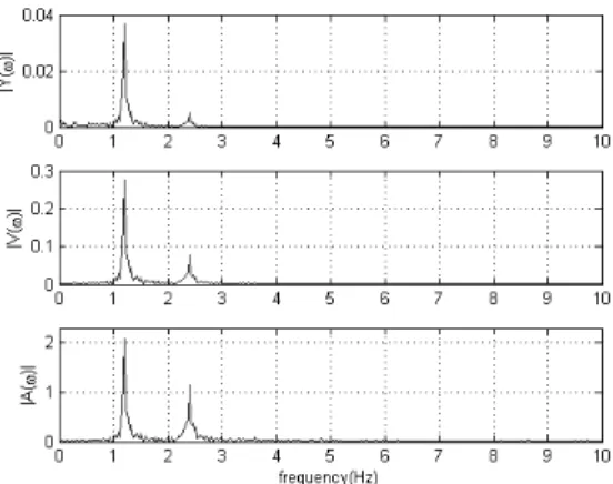
2.2 Analysis of the experimental data

Fast Fourier transforms of the recorded displacement, velocity, acceleration series show that the main

spectral component of these signals is at 1.2 Hz and the second order harmonic at 2.4 Hz. The

higher-order harmonic components are small. The spectrum of the displacement at the frequencies over 3

Hz is very smooth and the higher-order harmonics can hardly be observed. This is because the

displacement signal is integratal of the velocity and acceleration and the integrands have typical low

pass property. Since there is no external excitation in this autonomous system the harmonics in these

signals are introduced by nonlinearities.

Figure 2 The frequency spectra of the displacement, velocity, and acceleration signals

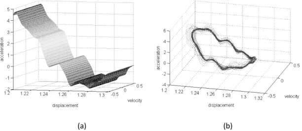
The nonlinearities can obviously be observed in the phase portrait of these signals which are shown

in Fig 3, especially in the acceleration- displacement phase plane in Fig 3 (c). The system is nonlinear

6 dimensional plane. Namely, the displacement

y t

 

y t

 

y t

 

a linear equation

0

my cy ky   (1)

Rearrangeing equation (1) yields

my  cy ky (2)

The right hand side of the equation represents the restoring force of a linear system composed of the

elastic force ky and the damping force cy, where

c

k

stiffness, respectively. Fig 3 (b) shows that the scattering of data in the three-dimensional state space

is flat in the acceleration direction which forms a surface in the state space. However the scattering

of the data is far from a plane. That is the data does not satisfy the linear relationship (1) but a

nonlinear one. A general form for nonlinear second order systems can be given as

 

,

my



f y y

where the internal restoring force is a nonlinear function of the displacement and the velocity.

Equation (3) shows the basic idea of the restoring force surface method (Masri & Caughey, 1979)

which will be used to identify the model of the system in the next section.

A further observation of Fig 3 (a), (d), and (b) shows that the phase portrait of the system is almost

symmetrical about the plane y0. That is the marked point moves at certain acceleration when the

displacement and the amplitude of velocity are specified disregarding the direction of the velocity.

Moreover, the change of acceleration along the velocity direction is insignificant. That is, the

directional derivative of the restoring force along the velocity is small. This means that the influence

of the velocity on the restoring force is insignificant and the restoring force mainly comes from a

nonlinear elastic force which is a function of displacement. As a result it is reasonable to assume that

the restoring force (or acceleration) does not depends on the value of the velocity and can be

described as a univariate function of displacement. This assumption simplifies the system

identification procedure in the next section. Under the above assumption the study of the restoring

force surface in a three dimensional state space reduces to a study of the nonlinear elastic restoring

force in the acceleration-displacement plane.

The nonlinear relationship between acceleration and displacement is shown in the projection of the

phase portrait on the acceleration-displacement plane. Fig 3 (c) shows that acceleration and

7 uniform nonlinear function in the whole phase plane. This nonlinear relationship will be studied in

next section using three different types of nonlinear terms: polynomial terms, multi-scale radial basis

functions, and the hybrid term set which combines the previous two kinds of terms.

(a) (b)

(c) (d)

Figure 3 Data in the phase space

3. Orthogonal forward regression restoring force surface method

T N

   

,

8 where

f y y



,



velocity. A trivial re-arrangement of equation (4) gives

 





1 1

,

y u t f y y

m m

  (5)

For a certain time instance t_i , a triplet y t

     

indicate a point in the phase plane and the third gives the height of the restoring force above that

point. The main idea of the restoring force surface method is to reconstruct the restoring force as a

function of velocity and displacement using measured force (or acceleration) and kinematic data at

discrete time instants.

In this paper, the orthogonal forward regression algorithm is employed to determine the structure of

the nonlinear restoring force surface. It is well known that the orthogonal forward regression

algorithm and the ERR criterion are very effective nonlinear system identification method and have

been successfully used to identify nonlinear systems in various applications. In this algorithm, a large

enough term dictionary is firstly constructed. Any type of linear and nonlinear terms and their

combination can be included in the candidate term set. The significant terms in the dictionary will be

selected into the final model one by one based on the ERR criterion until a stop criterion is satisfied.

The candidate terms are orthogonalised in each step to minimise the information redundancy in the

final model. The obtained models which include the least number of terms and possess a strong

descriptive power are often near to optimal.

By applying the orthogonal forward regression algorithm, various ranges of terms can be used to

recover the restoring force surface such as: polynomial terms, rational functions, radial basis functions,

wavelets functions, and so on, and also the hybrid models which combining different type of terms.

This will greatly extend the application of the restoring force surface method to the dynamic systems

with complex nonlinearities.

The new orthogonal forward regression restoring force surface method can then be summarised as:

(i) Design the experiment and prepare data. For example, select appropriate input signals to produce

good data for the next identification. Record all the displacement, velocity, and acceleration data or

obtain the data using a numerical integral or differentiation. This step is exactly same as the classical

restoring force surface method.

(ii) Construct a candidate term dictionary which should be large enough to cover all the correct

9 polynomials, wavelets, trigonometric functions, and so on. All these terms are function of either

displacement or velocity or both.

(iii) Apply the iOFR algorithm to select the significant terms from the dictionary and construct a

parsimony model.

(iv) Verify the obtained models using model validation methods or model perdition. A commonly used

model validation method is the high order correlation test method (S. A. Billings & Zhu, 1994; BlLlings

& Voon, 1986). Two kinds of predictions are often used for model validation: one-step-ahead

prediction and model predicted output. The model predicted output predicts the long term

behaviours of a system. A good model predicted output often means that the identify model can

represents the original system.

A very important issue encountered when applying the restoring force surface method is to design an

appropriate excitation signals. One of the important criteria is that the phase trajectory covers as

much of the phase plane as possible thus allowing one to construct a connected and continuous force

surface (S. Duym & Schoukens, 1995; Worden, 1990a). Therefore the restoring force surface method

is often used for the modelling of the nonlinear dynamical systems with external inputs. Directly

applying the restoring force surface method to an autonomous nonlinear system could be difficult(Y.

Guo, L. Z. Guo, S. A. Billings, & H.-L. Wei, 2015a). This is because the scattering points are sparse in a

three-dimensional state space for a nonlinear oscillation.

The nonlinear dynamics of the body motion which considered in this paper is autonomous and the

external force

u t

 

restoring force is a univariate function of displacement, equation (5) can then be written as

 

1

y f y

m

 (6)

This assumption makes the identification process enforceable since the data is sufficient for the

recovering of a restoring force curve in the two-dimensional displacement-acceleration plane (see fig

3 (c)) although the data scattering is sparse in a three dimensional state space.

It is worthy mentioning that this assumption seems not to be sufficiently supported because of the

sparseness of the data in the phase space. However, the identification results prove the correctness

of the assumption. That is a univariante restoring surface is adequate to represent the nonlinear body

10

4. Identification of the nonlinear oscillations

As what has been observed, the motion of the marked point in the vertical bouncing behaves as a

nonlinear oscillation. In this section, this nonlinear oscillation will be modelled using the new

introduced orthogonal forward regression restoring force surface method. Three different types of

candidate terms are used to represent the nonlinear system, including polynomial model, multi-scale

radial basis function model, and a hybrid model. The advantages and disadvantages of each model are

discussed in detail.

4.1 Identification of a polynomial model

Polynomial nonlinearities are widely used for the identification of nonlinear system because of the

inherent advantages of this kind of model. The nonlinear relationship between acceleration and the

displacement is firstly identified using this kind of model. Following the identification programme

given in section 3, a third order polynomial model is obtained. The identified model is given as follows

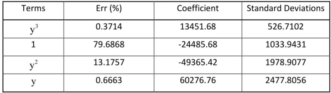
and the results are shown in Table 1. A total number of four terms are selected in the final model.

2 3

24485.68 60276.76 49365.42 13451.68

y   y y  y (7)

It can be observed that, using the iOFR algorithm, the first select term does not have a very large ERR,

which is different from the classic OFR algorithm. A less dominant first term may make the term

selection less greedy and a better model structure can be obtained (Yuzhu Guo, Guo, et al., 2015c). In

the obtained model the constant term produced the greatest ERR because the restoring force curve

does not go through the origin of the acceleration-displacement plane.

Table 1 The results of the forward regression

Terms Err (%) Coefficient Standard Deviations

3

y 0.3714 13451.68 526.7102

1 79.6868 -24485.68 1033.9431

2

y 13.1757 -49365.42 1978.9077

y 0.6663 60276.76 2477.8056

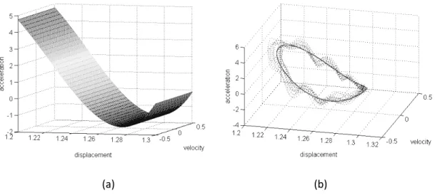
11 (a) (b)

Figure 4 Reconstruction of the restoring force surface using the polynomial model

Simulating the polynomial model, the comparison of the model predicted outputs with the

experimental data is shown in Fig 5. Details of the predicted acceleration signal are shown in Fig 6 by

zooming in Fig 5. Figure 4 (b) shows the predicated trajectory in the phase space. Figure 4, 5 and 6

show that the obtained polynomial model captures the main morphology of the experimental data

but misses some details.

12 Fig 6 Enlarged plot of the acceleration signal

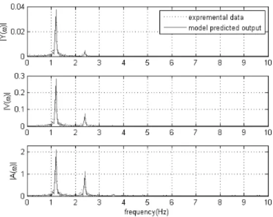
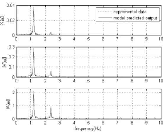
Fig 7 shows the comparison of the frequency spectra of the model predicted output and the

experimental data. It is shown that the simple polynomial model is capable to reproduce the basic

frequency component and the harmonics.

Fig 7 Frequency components of the model prediction output

The nonlinear terms in model (7) represent the nonlinear stiffness in the system, which plays a crucial

role in the generation of the harmonics. The polynomial models inherently possess many significant

advantages. (i) The polynomial model is of a very simple structure and easy to simulate and to realise

as a real physical system. (ii) Owing to the polynomial structure, the model can be easily used for

further analysis in both time and frequency domains. There are many mature techniques for the

analysis of systems with polynomial nonlinearities. For example, the perturbation method and

bifurcation analysis (Khalil, 2002), the describing function method (Kochenburger, 1950), and the

Volterra series theory and the associated generalised frequency response functions (Chua &

Yaw-Shing, 1982; Rugh, 1981). (iii) The output of the system is strictly harmonic signals. That is all the higher

frequencies are strict integer times of a basic frequency component.

However, problems start to occur when the restoring force surfaces are complex. This is simply

because the discontinuities and nonuniformities are very difficult to model using inherently smooth

polynomial terms. What make the condition worse is that the higher order polynomial model may

easily sink into the difficulty of instability. This is easy to explain. In order to satisfy the requirement

of a best fit some of the higher-order stiffness with negative coefficients may emerge in the final model

13

4.2 Radial basis function model

In order to characterise the system more accurately, radial basis functions are used as the term

dictionary of the iterative orthogonal forward regression restoring force surface method in this section.

Radial basis functions (RBF) whose value depends on the distance from the centre points can

efficiently characterise the position related local information. The radial basis functions should be a

good choice for the nonlinearity in this case.

The nonlinear restoring force surface is then represented as the linear combination of a series radial

basis functions



 

y

w

w

 

 

1 n

i i i

f y w









T G -scale radial basis functions.

2 2 2 ( ) i i x c

i x e





 

 (9)

where is the norm to define the distance from

x

According to the information show in the phase portrait the candidate term dictionary is constructed

as follows. The centres c_i choose values between 1.2 and 1.3 for every 0.001 unit where the limits of

the centres are determined by the phase plane trajectory. The scales



for every 0.001 unit to produce a sufficient cover to the range of the displacement, that is, the interval

[1.2, 1.3]. An appropriate choice of candidate term set is crucial for the identification process. A large

enough term set is needed to make sure that the underlying dynamics of the system can be well

approximated using the candidate model building blocks. However, a very large term set will make

the identification computationally intensive. The range of scales for the radial basis functions can be

efficiently determined through an iterative process. Initially, select a relatively small range of scales

in the dictionary and apply the orthogonal forward regression algorithm. Examine the obtained model

to check whether more than one RBF functions with the same centre but different scales are selected.

This often means that the dictionary is often not large enough because these RBF functions may be

approached by less RBFs of a larger scale. Enlarge the range of scales and repeat the process until this

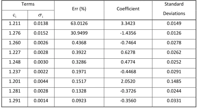
14 The iOFR algorithm is then employed to select the significant terms from the term dictionary. The

results are shown in Table 2. A total number of 9 terms are selected in the final model. These RBFs are

shown in Fig 8. Adding these weighted terms together yields the final model.

Table 2 Sub-models of the system

Terms

Err (%) Coefficient Standard Deviations

i

c



1.211 0.0138 63.0126 3.3423 0.0149

1.276 0.0152 30.9499 -1.4356 0.0126

1.260 0.0026 0.4368 -0.7464 0.0278

1.227 0.0028 0.3922 0.6278 0.0262

1.248 0.0030 0.3286 0.4774 0.0252

1.237 0.0022 0.1971 -0.4468 0.0291

1.201 0.0044 0.1517 2.0520 0.1485

1.281 0.0028 0.1328 -0.3726 0.0244

1.291 0.0014 0.0923 -0.3560 0.0331

15 The model predicted outputs are shown in Fig 9. The restoring force surface and the phase trajectory

are show in Fig 10 (a) and (b), respectively. It is easy to observe that the RBF model represents the

nonlinear restoring force better than the polynomial model did.

Figure 9 The model predicted outputs of the RBF model

(a) (b)

Figure 10 Reconstruction of the restoring force surface using the RBF model

The spectral analysis of the model predictions is shown in Fig 11. Although the RBF model prediction

fits the experimental data better in the time domain and in the state space, the polynomial model

prediction fits the data better in the frequency domain. There are more energy leaks around the

16 Figure 11 The spectra of the model prediction outputs of the RBF model

Fig 9, 10 and 11 show that the model predicted outputs agree with the experimental data. The results

show that the radial basis functions successfully overcome the divergence problem which may happen

in the high order polynomial model fitting. This shows the powerful fitting ability of the radial basis

function model. Theoretically, the multi-scale radial basis functions are able to recover any complex

restoring force surface and the multi-scale radial basis function approximations are asymptotically

optimal, in the sense of convergence rate (Stephen A. Billings et al., 2007). This means a parsimonious

model can be obtained.

However one obvious disadvantage of the method is that the model is unphysical and the coefficients

obtained for the expansion cannot directly yield information about the physical quantities in the

system, such as the damping and stiffness of the structure. Another disadvantage, which was shown

in the spectral analysis of the reproduced signals, is that the reproduced signals may have much richer

frequency components than a harmonic signal. This is not what expected because additional

frequency components which are not in the experimental data may be introduced through the RBF

model.

4.3 Hybrid model combining the polynomial and radial basis functions

According to the analysis in the previous sections, a model which possesses the advantages of both

the polynomial model and the radial basis function model is expected. That is, the hybrid model can

not only give an accurate description of the nonlinear dynamics but also accurately characterise the

system in frequency domain. In this section a two-level hybrid model will be identified to describe the

nonlinear oscillations in multi-scale from coarse to fine (Stephen A. Billings et al., 2007; Wei et al.,

17 A hybrid model which includes both polynomial and RBF terms were used to describe the dynamics.

The iOFR algorithm is again used to select the significant terms from the mixed term dictionary consists

of polynomial and RBF candidate terms. This time, the centres of the radial basis functions keep same

however the scales of the RBF terms are selected in a relatively smaller range from 0.0005 to 0.0030

to avoid the information overlap with the polynomial terms. This is because the hybrid model

represents the behaviours of the nonlinear system in two different levels. The polynomials recover

the main shape of the system and generate harmonic signals while the RBFs to characterise the local

details. Therefore, the scale of the RBFs is chosen to focus on the local information and shield off the

global information. While the polynomial terms characterise the large-scale information but neglect

the local details. The determination of an appropriate scale range for the RBFs is easy to realise in the

identification. Choose a relatively larger scale range, for example, the maximum scale in Table 2, and

set the initial range as 0.0005 ~ 0.0152. Reduce the upper limit and apply the orthogonal forward

regression algorithm until the polynomial terms start to appear in the model. In this example the scale

range is chosen as 0.0005 ~ 0.0030.

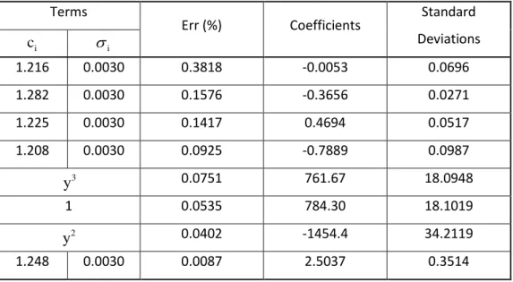
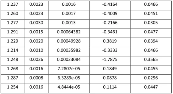
Apply the orthogonal forward regression algorithm and stop the forward selection process as the sum

of ERRs reaches 0.95 (Wei, Billings, & Liu, 2004). The obtained model structure and the associated

coefficients are given as Table 3. The list of the ERRs shows that the polynomial terms play important

roles in the final model. The comparison of the model predicted outputs and the real data is shown in

Fig 12. The comparison of the frequency spectra of the predicted outputs and the real data is show in

Fig 13. The results show that the model predicted outputs excellently agree with the experimental

data both in the time domain and also in frequency domain.

Table 3 Sub-models of the hybrid model

Terms

Err (%) Coefficients Standard Deviations

i

c



1.216 0.0030 0.3818 -0.0053 0.0696

1.282 0.0030 0.1576 -0.3656 0.0271

1.225 0.0030 0.1417 0.4694 0.0517

1.208 0.0030 0.0925 -0.7889 0.0987

3

y 0.0751 761.67 18.0948

1 0.0535 784.30 18.1019

2

y 0.0402 -1454.4 34.2119

18 1.237 0.0023 0.0016 -0.4164 0.0466

1.260 0.0023 0.0017 -0.4009 0.0451

1.277 0.0030 0.0013 -0.2166 0.0305

1.291 0.0015 0.00064382 -0.3461 0.0477

1.229 0.0020 0.00049928 0.3819 0.0394

1.214 0.0010 0.00035982 -0.3333 0.0466

1.248 0.0026 0.00023084 -1.7875 0.3565

1.268 0.0016 7.2807e-05 0.1849 0.0455

1.287 0.0008 6.3289e-05 0.0878 0.0296

1.254 0.0016 4.8444e-05 0.1114 0.0447

Figure 12 Model predicted output of the hybrid model

Figure 13 Spectra of the model predicted output of the hybrid model

However the hybrid model has not shown significant advantages over the RBF model so far. It is

expected that the polynomial part of the hybrid model can also give an acceptable description of the

19 three polynomial terms in the hybrid model is exactly same as the first three terms in the purely

polynomial model.

Extracting the polynomial terms from the hybrid model yields a new polynomial model as

2 3

784.30 1454.4 761.67

y  y  y (10)

Plot the hybrid model and the extracted polynomial model (10) in the displacement-acceleration

phase plane. Fig 14 shows that model (10) fits the experimental data very well.

Fig 14 The fitness of the hybrid model in the displacement-acceleration phase plane

The model predicted output of the polynomial part (model(10)) and the spectra of the prediction are

shown in Fig 15 and 16 respectively. Although the model predicted outputs do not fit the data very

well after 6 seconds the model predictions perfectly reproduced the frequency spectra of the

experimental data, which is even better than the pure polynomial model (7) did. This means that the

polynomial part of the hybrid model is capable to represent the global behaviours neglecting some

local details. This is because the Fourier transform always gives average information of the whole time

20 Fig 15 The model predicted output of the polynomial part

Fig 16 Spectra of the model predicted outputs by model (10)

To sum up, the hybrid model successfully provides a two-level coarse-to-fine, representation of the

nonlinear systems. The polynomial terms give a coarse description which could characterise the main

frequency components of the nonlinear oscillations whereas the complete model gives a more

accurate description of both the local and global behaviours of the system.

5. Conclusions

The nonlinear oscillations existing in human bouncing has been investigated. A new system

identification method which combines the restoring force method and the iterative orthogonal

forward regression algorithm has been introduced. The system identification based method which

avoids the difficulties in a first principle method is simple to carry out in the practical applications.

The obtained models have been shown to be able to reproduce the nonlinear oscillation both in the

time and frequency domain. The new identification method itself extends the restoring force method

to a more wide class of system with complex nonlinearities. Although a special example where the

external input is zero and the effect of the velocity can be ignored has been studied in this paper this

does not prevent the new orthogonal forward regression restoring force surface method to be a

21

References

Allen, M. S., Sumali, H., & Epp, D. S. (2008). Piecewise-linear restoring force surfaces for semi-nonparametric identification of nonlinear systems. Nonlinear Dynamics, 54(1-2), 123-135. doi:10.1007/s11071-007-9254-x

Billings, S. A. (2013). Nonlinear System Identification : NARMAX Methods in the Time, Frequency, and Spatio-Temporal Domains. Hoboken, New Jersey: John Wiley & Sons Ltd.

Billings, S. A., Wei, H.-L., & Balikhin, M. A. (2007). Generalized multiscale radial basis function networks.

Neural Networks, 20(10), 1081-1094. doi:https://doi.org/10.1016/j.neunet.2007.09.017

Billings, S. A., & Wei, H. L. (2005). The wavelet-NARMAX representation: a hybrid model structure combining polynomial models with multiresolution wavelet decompositions. Intern. J. Syst. Sci., 36(3), 137-152. doi:10.1080/00207720512331338120

Billings, S. A., & Zhu, Q. M. (1994). Nonlinear model validation using correlation tests. International Journal of Control, 60(6), 1107-1120.

Blickhan, R. (1989). The spring-mass model for running and hopping. J Biomech, 22(11-12), 1217-1227. BlLlings, S. A., & Voon, W. S. F. (1986). Correlation based model validity tests for non-linear models.

International Journal of Control, 44(1), 235-244. doi:10.1080/00207178608933593

Chua, L., & Yaw-Shing, T. (1982). Nonlinear oscillation via Volterra series. Circuits and Systems, IEEE Transactions on, 29(3), 150-168. doi:10.1109/tcs.1982.1085129

Duym, S., & Schoukens, J. (1995). Design of excitation signals for the restoring force surface method.

Mechanical Systems and Signal Processing, 9(2), 139-158. doi:http://dx.doi.org/10.1006/mssp.1995.0012

Duym, S. W. R., Schoukens, J. F. M., & Guillaume, P. A. N. (1996). A local restoring force surface method.

Modal Analysis-the International Journal of Analytical and Experimental Modal Analysis, 11 (3-4), 116-132.

Ernesto, D., & Tianjian, J. (2009). Action of Individual Bouncing on Structures. doi:10.1061/(ASCE)0733-9445(2009)135:7(818)

Garcia, M. S. (1999). Stability scaling and chaos in passive-dynamic gait models. (Ph.D.), Cornell University.

Guo, Y., Guo, L. Z., Billings, S. A., & Lang, Z. Q. (2015). A New Efficient System Identification Method for Nonlinear Multiple Degree-of-Freedom Structural Dynamic Systems. Journal of Computational and Nonlinear Dynamics, 11(2), 021012-021012. doi:10.1115/1.4031488 Guo, Y., Guo, L. Z., Billings, S. A., & Wei, H.-L. (2015a). Identification of nonlinear systems with

non-persistent excitation using an iterative forward orthogonal least squares regression algorithm.

International Journal of Modelling, Identification and Control, 23(1), 1-7. doi:10.1504/ijmic.2015.067496

Guo, Y., Guo, L. Z., Billings, S. A., & Wei, H.-L. (2016). Identification of continuous-time models for nonlinear dynamic systems from discrete data. International Journal of Systems Science, 47(12), 3044-3054. doi:10.1080/00207721.2015.1069906

Guo, Y., Guo, L. Z., Billings, S. A., & Wei, H. L. (2015b). Identification of linear systems with non-persistent excitation using an iterative forward orthogonal least squares regression algorithm.

International Journal of Modelling, Identification and Control, 23(1), 1-7.

Guo, Y., Guo, L. Z., Billings, S. A., & Wei, H. L. (2015c). An iterative orthogonal forward regression algorithm. Int. J. Syst. Sci., 46(5), 776-789. doi:10.1080/00207721.2014.981237

Guo, Y., Storm, F., Zhao, Y., Billings, S. A., Pavic, A., Mazza, C., & Guo, L. Z. (2017). A New Proxy Measurement Algorithm with Application to the Estimation of Vertical Ground Reaction Forces Using Wearable Sensors. Sensors (Basel), 17(10). doi:10.3390/s17102181

22 Hof, A. L., Van Zandwijk, J. P., & Bobbert, M. F. (2002). Mechanics of human triceps surae muscle in walking, running and jumping. Acta Physiologica Scandinavica, 174(1), 17-30. doi:10.1046/j.1365-201x.2002.00917.x

Khalil, H. K. (2002). Nonlinear Systems (3rd ed ed.). London: Prentice Hall.

Kochenburger, R. J. (1950). A Frequency Response Method for Analyzing and Synthesizing Contactor Servomechanisms. American Institute of Electrical Engineers, Transactions of the, 69(1), 270-284. doi:10.1109/t-aiee.1950.5060149

Masri, S. F., Bekey, G. A., Sassi, H., & Caughey, T. K. (1982). Non-parametric identification of a class of nonlinear multidegree dynamic systems. Earthquake Engineering & Structural Dynamics, 10(1), 1-30. doi:10.1002/eqe.4290100102

Masri, S. F., & Caughey, T. K. (1979). A Nonparametric Identification Technique for Nonlinear Dynamic Problems. Journal of Applied Mechanics, 46(2), 433-447.

Racic, V., & Chen, J. (2015). Data-driven generator of stochastic dynamic loading due to people bouncing. Computers & Structures, 158, 240-250. doi:http://dx.doi.org/10.1016/j.compstruc.2015.04.013

Racic, V., & Pavic, A. (2010a). Mathematical model to generate near-periodic human jumping force signals. Mechanical Systems and Signal Processing, 24(1), 138-152. doi:http://dx.doi.org/10.1016/j.ymssp.2009.07.001

Racic, V., & Pavic, A. (2010b). Stochastic approach to modelling of near-periodic jumping loads.

Mechanical Systems and Signal Processing, 24(8), 3037-3059. doi:http://dx.doi.org/10.1016/j.ymssp.2010.05.019

Racic, V., Pavic, A., & Brownjohn, J. M. W. (2009). Experimental identification and analytical modelling of human walking forces: Literature review. Journal of Sound and Vibration, 326(1 ?), 1-49. doi:http://dx.doi.org/10.1016/j.jsv.2009.04.020

Rugh, W. J. (1981). Nonlinear System Theory: The volterra/Wiener Approach. London: Johns Hopkins University Press.

Spägele, T., Kistner, A., & Gollhofer, A. (1999a). Modelling, simulation and optimisation of a human vertical jump. Journal of Biomechanics, 32(5), 521-530. doi: http://dx.doi.org/10.1016/S0021-9290(98)00145-6

Spägele, T., Kistner, A., & Gollhofer, A. (1999b). A multi-phase optimal control technique for the simulation of a human vertical jump. Journal of Biomechanics, 32(1), 87-91. doi:http://dx.doi.org/10.1016/S0021-9290(98)00135-3

van Werkhoven, H., & Piazza, S. J. (2013). Computational model of maximal-height single-joint jumping predicts bouncing as an optimal strategy. Journal of Biomechanics, 46(6), 1092-1097. doi:http://dx.doi.org/10.1016/j.jbiomech.2013.01.016

Wei, H. L., Billings, S. A., & Liu, J. (2004). Term and variable selection for non-linear system identification. International Journal of Control, 77(1), 86-110. doi:10.1080/00207170310001639640

Wei, H. L., Zhu, D. Q., Billings, S. A., & Balikhin, M. A. (2007). Forecasting the geomagnetic activity of the Dst index using multiscale radial basis function networks. Advances in Space Research, 40(12), 1863-1870. doi:https://doi.org/10.1016/j.asr.2007.02.080

Worden, K. (1990a). Data-processing and experiment design for the restoring force surface method, part II. choice of excitation signal. Mechanical Systems and Signal Processing, 4(4), 321-344. doi:10.1016/0888-3270(90)90011-9

Worden, K. (1990b). Data processing and experiment design for the restoring force surface method, part I: integration and differentiation of measured time data. Mechanical Systems and Signal Processing, 4(4), 295-319. doi:http://dx.doi.org/10.1016/0888-3270(90)90010-I