Characterization of the effects of the human head on communication with implanted antennas

(1)

Rochester Institute of Technology

RIT Scholar Works

Theses Thesis/Dissertation Collections

2010

Characterization of the effects of the human head

on communication with implanted antennas

Michael A. Pecoraro

Follow this and additional works at:http://scholarworks.rit.edu/theses

This Thesis is brought to you for free and open access by the Thesis/Dissertation Collections at RIT Scholar Works. It has been accepted for inclusion in Theses by an authorized administrator of RIT Scholar Works. For more information, please [email protected].

Recommended Citation

(2)

CHARACTERIZATION OF THE EFFECTS

OF THE HUMAN HEAD ON COMMUNICATION

WITH IMPLANTED ANTENNAS

by

Michael A. Pecoraro

A Thesis Submitted in Partial Fulfillment of the Requirements for the Degree of

MASTER OF SCIENCE in

Electrical Engineering Approved by:

Professor_______________________________________ (Dr. Jayanti Venkataraman – Advisor)

Professor_______________________________________ (Dr. Sohail Dianat – Advisor)

Professor_______________________________________ (Dr. Gill Tsouri – Advisor)

Professor_______________________________________ (Dr. Lynn Fuller – Committee Member)

Professor_______________________________________ (Dr. Sohail Dianat – Department Head)

DEPARTMENT OF ELECTRICAL AND MICROELECTRONIC ENGINEERING KATE GLEASON COLLEGE OF ENGINEERING

ROCHESTER INSTITUTE OF TECHNOLOGY ROCHESTER, NEW YORK

(3)

Acknowledgement

This work could never have been completed without the help of others... That being said, I would like to dedicate this to…

Dr. Venkataraman –

who has guided me through my entire career here at RIT and whose only fault seems to be that she prefers Roger Federer over Andy Roddick… which I can forgive

Dr. Dianat and Dr. Tsouri – who are always ready to answer questions, help me and tell me, honestly, what they think

Jim Stefano, Ken Synder, Patti Vicari, Florence Layton and the E& E Department – who helped me with everything from scheduling things, getting Post-it notes, printing, scanning,

fixing license problems, scheduling more things, booking rooms… on and on, ad infinitum

My Family – Mom, Dad, Megan, Joe and Steve – who support me in everything I do,

and love me as much as I love them

My Friends – Zachary, Ben, Toni and Chad – who kept me sane, listened to me rant,

made me laugh and so much more

(4)

Thesis Release Permission

DEPARTMENT OF ELECTRICAL AND MICROELECTRONIC ENGINEERING

COLLEGE OF ENGINEERING

ROCHESTER INSTITUTE OF TECHNOLOGY ROCHESTER, NEW YORK

FEBRURARY 2010

Title of Thesis:

CHARACTERIZATION OF THE EFFECTS

OF THE HUMAN HEAD ON COMMUNICATION

WITH IMPLANTED ANTENNAS

I, Michael Pecoraro, hereby grant permission to Wallace Memorial Library of the Rochester Institute of Technology to reproduce this thesis in whole or in part. Any

reproduction will not be for commercial use or profit.

(5)

(6)

i

ABSTRACT

Cranially implanted sensors and electrodes have been used in practice for several years;

their applications range from the recording of neural signals for use in Brain-Computer

Interfaces to help the disabled, to the treatment of diseases and conditions ranging from

Parkinson‟s disease, multiple sclerosis, depression, etc. Current communication methods with

implants, however, are lacking; they run the gamut from physical, percutaneous connections that

increase the risk of infection, to wireless links that are slow and uncomfortable for patients.

The present work focuses on the characterization of the effects of the human head on

communication with cranially implanted antennas for its eventual use in improving current

communication methods. A realistic human head model with frequency dependent tissue

characteristics is used to obtain a transfer function that describes the magnitude and phase of an

electromagnetic wave as it propagates through the human head over both frequency and depth

into the skull; this data is obtained for multiple energy entry angles. The technique used to obtain

transfer function measurements consists of taking the ratio of the electric fields at the receiver

and transmitter and is developed through analysis of ultra-wideband transmit/receive antenna

systems; verification for this technique is provided.

After the transfer function data described above is obtained, we posit a communication model

to approximate the transfer function magnitude. This approximation takes the form of a modified

log-distance, log-frequency path loss model and fits the data quite well. The final approximation

describes the path loss of an electromagnetic wave over both frequency and distance for all

simulated orientations.

Lastly, simulations are presented for communication from a cranially implanted dipole

(7)

ii

(from the head), as well as location (around the head) – is captured and plotted. We finally show

that the transfer function that was obtained for all perpendicular communication through the head

(8)

iii

LIST OF FIGURES

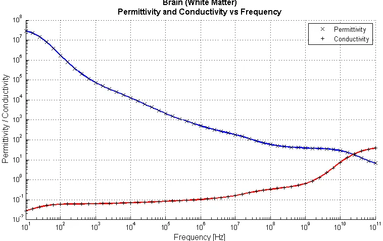
Figure 1: Permittivity and Conductivity of Brain (White Matter) vs. Frequency ... 15

Figure 2: Permittivity and Conductivity of Bone (Cancellous) vs. Frequency... 16

Figure 3: Permittivity and Conductivity of Muscle vs. Frequency ... 16

Figure 4: Images of the Human Body Model, Front and Side Views ... 19

Figure 5: Conventional Ultra-wideband Transmit-Receive Antenna System ... 23

Figure 6: Transfer Function of the Channel, as a part of the Total System Transfer Function .. 24

Figure 7: UWB Sub-System 1: Transmit Antenna and Channel... 25

Figure 8: UWB Sub-System 2: Receive Antenna ... 25

Figure 9: UWB Sub-System 2, Reversed: Transmit Antenna ... 26

Figure 10: Channel Transfer Function, in terms of E-Fields ... 27

Figure 11: E-Field Verification Simulation Setup ... 28

Figure 12: Time Domain Electric Field Probe Measurements, Free Space ... 29

Figure 13: Theoretical/Calculated Transfer Function Comparison, Free Space ... 29

Figure 14: Time Domain Electric Field Probe Measurements, Approximate Head Values ... 30

Figure 15: Theoretical/Calculated Transfer Function Comparison, Approximate Head Values 31 Figure 16: Setup for E-Field Simulations, Probes and Plane Wave ... 32

Figure 17: General Dimensions of the Human Body Model for E-Field Simulation ... 33

Figure 18: Axial Cross-Sections of the Human Head Model ... 34

Figure 19: Time Domain Input E-Field Signal, Gaussian Pulse... 35

Figure 20: Frequency Domain Input E-Field Signal, FFT of the Gaussian Pulse ... 36

Figure 21: Time Domain Reference E-Field Signal, Left Side of the Head ... 36

(13)

viii

Figure 23: Frequency Domain Reference E-Field Signal, Left Side of the Head ... 38

Figure 24: Frequency Domain E-Field Signals, Depths of 3cm, 5cm, 7cm, Left Side of the Head ... 38

Figure 25: Transfer Function Magnitude, 2:1:8cm, Left Side of the Head ... 40

Figure 26: Offset Coordinate System Dimensions for Different Incidence Angles ... 41

Figure 27: Transfer Function Magnitude, 2:1:8cm, Back of the Head ... 42

Figure 28: Transfer Function Magnitude, 2:1:8cm, Front of the Head ... 42

Figure 29: Transfer Function Magnitude, 2:1:8cm, Top of the Head ... 43

Figure 30: 3D Comparison Between E-Field Ratio and Poynting Vector Techniques ... 45

Figure 31: Comparison Between E-Field Ratio and Poynting Vector Techniques ... 46

Figure 32: Transfer Function Phase vs. Frequency, From Left, Back, Top and Front, Distances of 2cm:1cm:8cm ... 47

Figure 33: Transfer Function Phase vs. Distance, From Left, Back, Top and Front, Frequencies of 300MHz:100MHz:3000MHz ... 48

Figure 34: Simple Example of Linear Curve Fitting ... 49

Figure 35: Simulated and Estimated Curves, Simple Linear Fit ... 53

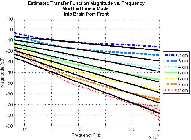
Figure 36: Simulated and Estimated Curves, Modified Linear Fit ... 55

Figure 37: Simulated and Estimated Curves, Indoor Propagation Model ... 58

Figure 38: Simulated and Estimated Curves, Modified Indoor Propagation Model ... 60

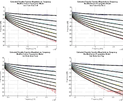
Figure 39: Simulated and Estimated Curves for Modified Indoor Propagation Model, All Angles ... 61

Figure 40: Simulated and Estimated Curves for Total Modified Indoor Propagation Model ... 62

(14)

ix

Figure 42: Spherical Six-Layered Head Model Used by Kim and Rahmat-Samii ... 67

Figure 43: Maximum Available Power Obtained at an Exterior Dipole Antenna from an Internally Implanted Dipole ... 68

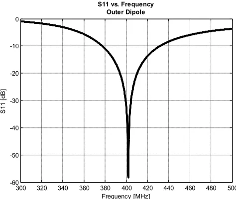
Figure 44: Return Loss Plot, External Dipole ... 70

Figure 45: External Dipole, Radiation Pattern, Simulated Farfield Parameters ... 70

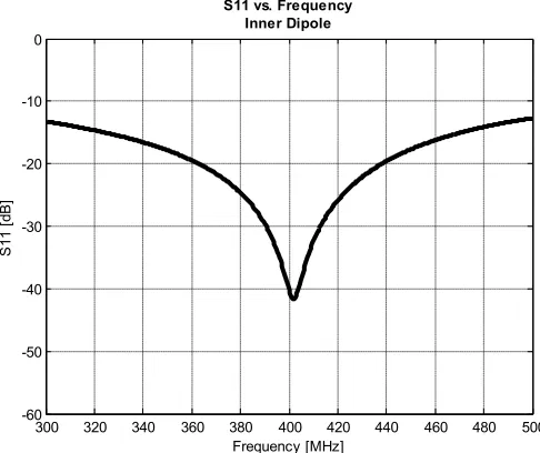
Figure 46: Return Loss Plot, Internal Dipole ... 71

Figure 47: Communication Link Simulation, Distance From External Dipole to Center, 1m ... 71

Figure 48: Communication Link Simulation, Distance From External Dipole to Center, 1m. Comparison to Results from Kim and Rahmat-Samii ... 73

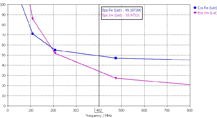
Figure 49: and for Brain, as defined in Kim and Rahmat-Samii’s Paper ... 75

Figure 50: and for Brain, as defined by Ansoft Corporation’s Human Body Model ... 76

Figure 51: General Dimensions of the Human Body Model for Antenna Simulations ... 77

Figure 52: General Setup of Distance Power Level Simulation with Centered Inner Dipole ... 78

Figure 53: General Setup of Distance Power Level Simulation with Off-Center Inner Dipole ... 78

Figure 54: Maximum Available Power vs. Distance, Human Head Model, Centered and Off-Centered Inner Dipole. Comparison vs. Kim and Rahmat-Samii’s Simplified Model. ... 80

Figure 55: Maximum Available Power vs. Distance, Centered Internal Dipoles for Human Head Model with both Body Model Brain Epsilon and the Simpler Kim and Rahmat-Samii Brain Epsilon, Comparison vs. Kim and Rahmat-Samii’s Simplified Model. ... 82

Figure 56: General Setup of Rotational Power Level Simulation with Centered Inner Dipole ... 84

Figure 57: Maximum Available Power vs. Angle, Human Head Model, Centered, d = 25, 50cm ... 85

(15)

x

Figure 59: Maximum Available Power vs. Angle, Human Head Model, Centered vs. Off-Center,

d = 50cm ... 87

Figure 60: Maximum Available Power vs. Distance, Human Head Model, Centered and Off-Centered Inner Dipoles, Replotted ... 90

Figure 61: Line-of-Sight Tissue Distances for Centered and Off-Center Inner Dipoles ... 90

Figure 62: Predicted Power Losses for 400MHz vs. Distance, One Distance Prediction ... 91

Figure 63: Three Predictions: Side to Front, Side to Back, Front to Back ... 92

Figure 64: Maximum Available Power vs. Angle, Human Head Model, Centered, d = 25, 50cm, Replotted ... 92

Figure 65: Predicted Power Losses for 400MHz vs. Distance, Three Rotation Predictions ... 93

Figure 66: Line-of-Sight Tissue Distances for an Off-Center Inner Dipole ... 93

Figure 67: Maximum Available Power vs. Angle, Human Head Model, Centered vs. Off-Center, d = 50cm, Replotted ... 94

Figure 68: Predicted Power Losses for 400MHz vs. Distance, One Rotation Prediction ... 94

Figure 69: Near Field Effect Simulation, Centered Internal Dipole, ... 97

Figure 70: Internal Communication Setup, 3D to 2D E-Field Result at 135 degrees ... 98

Figure 71: External Communication Setup, 3D to 2D E-Field Result at 337.5 degrees ... 99

Figure 72: SAR Simulation Setup and Result ... 101

Figure 73: SAR Simulation Results, External Antenna as Transmitter ... 103

Figure 74: (A) Exposed human brain after craniotomy (B) 8x8 ECoG sensor grid placed on the human brain (C) X-Ray image of a human skull with ECoG sensor grid (D) Average brain template with electrode locations highlighted ... 106

(16)

xi

Figure 76: Simulated and Estimated Curves, 2:1:8cm, 2nd Order Polynomial Fit, Left... 115

Figure 77: Simulated and Estimated Curves, 2:1:8cm, 2nd Order Polynomial Fit, Back ... 116

Figure 78: Simulated and Estimated Curves, 2:1:8cm, 2nd Order Polynomial Fit, Front ... 116

Figure 79: Simulated and Estimated Curves, 2:1:8cm, 2nd Order Polynomial Fit, Top... 117

Figure 80: Simulated and Estimated Curves, 2:1:8cm, Modified 2nd Order Polynomial Fit, Left ... 118

Figure 81: Simulated and Estimated Curves, 2:1:8cm, Modified 2nd Order Polynomial Fit, Back ... 119

Figure 82: Simulated and Estimated Curves, 2:1:8cm, Modified 2nd Order Polynomial Fit, Front ... 119

(17)

xii

LIST OF TABLES

Table 1: Possible Channel Types with Respect to Human Body Communication ... 7

Table 2: Electrical Characteristics of Several Relevant Body Tissues at 400MHz ... 35

Table 3: MMSE Variables and Ave Error for Simple Linear Model, From Front ... 52

Table 4: MMSE Variables and Ave Error for Simple Linear Model, All Angles ... 53

Table 5: MMSE Variables and Ave Error for Modified Linear Model, From Left ... 54

Table 6: MMSE Variables and Ave Error for Modified Linear Model, All Angles ... 55

Table 7: MMSE Variables and Ave Error for Simple Indoor Propagation Model, From Left .... 58

Table 8: MMSE Variables and Ave Error for Simple Indoor Propagation Model, All Angles .... 59

Table 9: MMSE Variables and Ave Error for Modified Indoor Propagation Model, From Left . 60 Table 10: MMSE Variables and Ave Error for Modified Indoor Propagation Model, All Angles ... 61

Table 11: MMSE Variables and Ave Error for Total Modified Indoor Propagation Model ... 62

Table 12: Electrical Data of Biological Tissues Used by Kim and Rahmat-Samii ... 67

Table 13: External Dipole Dimensions, Variables ... 69

Table 14: Internal Dipole Dimensions, Variables ... 71

Table 15: Electrical Data of Biological Tissues Used in Kim and Rahmat-Samii’s Spherical Head Simulations at 402MHz ... 74

Table 16: Tissue Densities Used by Kim and Rahmat-Samii for SAR Calculation ... 102

(18)

1

1. Introduction

1.1 Electromagnetic Wave Propagation and the Human Body

The biological effects of microwave radiation have been of interest for many years. It is

necessary, then, to have accurate data concerning the electrical properties of such biological

tissue. Since the 1960s much work has been done to compile this data for many different types of

tissue, both animal and human, over large frequency ranges [1]–[3], [5], [6], [8]–[12]. This type

of data acquisition is known as dielectric spectroscopy.

Historically, several different methods have been used to perform dielectric spectroscopy.

One method, used often in the burgeoning years of this research, was the use of sample

terminated transmission lines [6] [8]. A rectangular waveguide, or equivalent transmission line,

would be terminated with a sample of the tissue-under-test and a short circuit. Measurement of

the reflection coefficient could then be used to obtain the permittivity and conductivity of the

sample. This first method provides accurate measurements in the 100MHz to 1GHz region, but

fails to obtain accurate values at higher frequencies.

A second method, the use of an open-ended coaxial probe, soon became popular because

of its ability to make accurate measurements over a wide range of frequencies with little

overhead in preparation of the sample [2] [3] [5] [10] [11]. The popularity of this method was

helped, in part, by the development of more advanced and accurate network analyzers and

impedance analyzers. The technique is based on the fact that an open-ended probe has a fringing

capacitance and conductance that can be determined solely based on the geometry of the probe

and can be measured by a network/impedance analyzer. It is then possible to obtain the complex

(19)

2

line itself and the impedance of the line when it is in contact with a sample of unknown electrical

characteristics. This method has been used by many researchers to obtain data for biological

tissues up to 100GHz. This method, however, is not without its drawbacks. The inherent

inhomogeneity of tissue can provide different measured values depending on the placement of

the probe on the tissue. Also, problems such as electrode polarization, which is the manifestation

of charges that occur at the interface of the sample and the probe, can influence the results that

are obtained at the higher ends of the frequency spectrum. There are measurement techniques,

however, that can minimize the effect of this type of systematic error [4]. Improvements to this

method of dielectric spectroscopy are even now being developed. The necessity for in vivo

dielectric measurements yielded the design of a new probe in 2005. This probe was a

hermetically sealed coaxial probe that was bio-compatible and able to withstand harsh

sterilization procedures and is therefore able to be used in hospital environments for both in vivo

and ex vivo measurements.

The best known compilation of complex permittivity data for biological tissues is

contained in a three paper series from 1996 by Gabriel et al [1]–[3]. The open-ended coaxial

probe technique was utilized to obtain the permittivity and conductivity of seventeen different

human tissue types (blood, cortical bone, white matter, heart, liver, skin, etc.) over a frequency

range of 10Hz to 100GHz. Gabriel et al., in this series, also summarizes and presents results from

other papers for other tissues.

As would be expected of any material over such a wide range of frequency, material

properties do not stay constant, but actually vary with the frequency of energy that is applied.

This behavior is known as dispersion, and biological tissues actually exhibit multiple dispersion

(20)

3

and relaxation mechanisms inherent in the cellular and molecular makeup of the tissue [1] [13].

The first region, the alpha dispersion region, occurs at low frequencies and is associated with

counterion effects near membrane surfaces. The beta dispersion region, which is in the frequency

range of hundreds of kilohertz, is due to the effects of macromolecules within the cellular

membranes. The gamma dispersion region, in the gigahertz region, is mainly due to dipolar

mechanisms of water, salt and proteins. These regions all work together to, as frequency

increases, decrease the permittivity and increase the conductivity of any tissue in an uneven,

step-like fashion which has been attempted to be described using two main types of

mathematical models; the Debye model and the Cole-Cole model [4]. These models, which will

be elaborated on later, use either single or multiple time constants that can be either relaxed or

tightened to approximate the unique curves exhibited by each individual tissue. Several different

methods have been used to determine the optimum values for the time constants including least

squares analysis, approximation using MATLAB functions and even a brute force method, used

by Gabriel et al., to obtain a “…good fit to the data rather than a unique solution based on a

mathematical argument.” [15] [7] [3]

Much of the data that has been collected to this day is being used in the simulation of

medical devices that have been implanted in the human body. These simulations are

investigating what effects the layers of frequency dependent materials (presented by tissue) have

on the propagation of the electromagnetic waves inside and outside of the body. Thus far,

research in this area has focused on antennas; either in their design or in their effects on the

tissue around them (Specific Absorption Rate). Some efforts have also been applied to

developing new techniques that will be able to obtain, in vivo, the complex permittivities of

(21)

4

The area of medical implant antenna design is a relatively new field and has seen an

influx of research in the past ten years not only because of the usefulness of such devices, but

because of the allocation of specific frequency bands for such devices. The main band of interest

is the Medical Device Radiocommunications Service (also known as MedRadio). MedRadio is

an ultra-low power, unlicensed, mobile radio service for transmitting data in support of

diagnostic or therapeutic functions associated with implanted and body-worn medical devices.

This frequency band, previously known as the Medical Implant Communications Service band

(MICS), was established in 1999 by the FCC to overcome the limitations of the previous

biotelemetry techniques. These techniques were dependent on magnetic coupling for data

transfer. This meant that the external monitoring equipment would have to be very close to the

patient, often making contact with the skin and the equipment could only provide low data rates.

Comparatively, MedRadio allows for high-speed, reliable, short-range (up to 2m), wireless links

with implants. These improvements look to improve patient quality of life, reduce the risk of

infection, enhance patient comfort and expand freedom of movement for both the patient and

medical personnel [16] [17]. The MedRadio band itself is the frequency range of 401-406MHz.

Operation in this range has a bandwidth limitation of 300kHz and an effective isotropic radiated

power (EIRP) of -16dBm or lower [17] [19]. The range of 401-406MHz was selected

for several reasons, not least of which is that these frequencies have propagation characteristics

conducive to the transmission of radio signals within the human body. This will allow for the

constraints of power, size and antenna performance to be more easily met. In addition, this range

is internationally accepted in such areas as Europe/the UK, Canada, New Zealand, Korea and

(22)

5

Other frequency ranges also have the ability to transmit medical data. The WMTS

(Wireless Medical Telemetry) band, established by the FCC in 2000, allows for the remote

monitoring of a patient‟s health in the 608-614MHz, 1395-1400MHz and 1427-1432MHz

ranges. Applications here include devices that measure vital signs (pulse, respiration rates), etc

[21]. There are Industrial, Scientific and Medical bands that have also been used for medical

communication, although these frequency bands are much more crowded with other possible

uses. These so-called ISM bands are in the 900MHz and 2400MHz regions [22] [23]. Lastly, the

FCC is, as of August 2009, debating whether or not to add more frequency allocations for new

Medical Micro-Power networks. MMNs are currently defined as a network of multiple (from 1

to 100) micro-medical implants connected by an external controller that can be used as sensors to

provide information or can provide electrical stimulation to ease neurological conditions that

cause pain and suffering – polio, multiple sclerosis, stroke or brain injury, for example. The

proposed frequency ranges make up 24MHz of bandwidth over the multiple ranges of

413-419MHz, 426-432MHz, 438-444MHz and 451-457MHz [32].

Using the allocated frequency bands as a jumping off point, many researchers began

designing antennas for medical implants, the most popular of which seems to be variations on

Planar Inverted-F Antennas (PIFAs). Meandering dipole PIFAs have been designed for the use

with cardiac pacemakers. These have package sizes of 32x40mm or 36x40mm and use

superstrates to shield the antennas from the detuning effects of the body. Simulations have

shown these antennas to obtain return losses of 17 to 22dB down, and return losses in a fluid that

approximates the characteristics of human tissue, 5 to 8dB down. Both the far field radiation

(23)

6

Further work was done to modify the widths of the striplines to show improved radiation

performance and reduced maximum SAR values [25].

More PIFA antennas were designed in both spiral and serpentine configurations. These

antennas were also designed specifically for use with pacemakers and were simulated as such in

simplified and detailed human body models. These antennas had many variables tuned including

superstrate permittivity, substrate permittivity, stripline lengths, feed locations, ground point

locations, superstrate heights, superstrate geometries, etc. Simulated results show good matches

in the 400MHz range [26].

More antenna design has been done regarding stacking circular PIFA antennas to

decrease antenna size, enhance bandwidth and reduce detuning effects of the body. Simulations

show that return losses of greater than 30dB down can be achieved [27]. SAR studies, radiation

patterns and efficiency have also been explored for this antenna type. Other antenna designs have

been attempted as well. Simple wire antennas for use in pacemakers, encapsulated planar loop

antennas at the 900MHz ISM band and also patch antennas [28]–[31]. Some patch antenna

designs have used genetic algorithms to miniaturize the patches and obtain matches of anywhere

from 18 to 35 dB down, and some patch antennas have been designed at higher frequencies

(31.5GHz) to obtain an attractive form factor.

Other work with antennas has investigated the effects of body shape and body position on

the radiation pattern. Gain differences have shown to vary as much as 10dB based on the age,

sex, and arm position of the models [28], [32]–[34].

Further work can, and has been done to analyze the effects of the implanted antennas on

the tissue that surrounds it. Specific Absorption Rate (SAR) is the power that is absorbed by

(24)

7

regulations on SAR; for mobile phone certification the limit is 1 W/kg over 1g [28]. Several of

the papers that presented antenna designs also evaluated the SAR levels of their respective

antennas [24]–[26].

A final note on work that has been done in the area of electromagnetics and the human

body is the work done on tissue characterization [14]. The major goal of this work is to use

microwaves to detect cancer in the human body. It is known that tumors and healthy tissue have

very different electrical properties [12] [37]. Much of this difference arises from the fact that

tumors have a much higher water content that healthy tissue and thereby have increased loss.

Research has been done in the area of antenna design and near-field image methods to

effectively determine permittivity profiles of a possibly cancerous area [35]–[37].

1.2 Communication Issues and the Human Body

Turning to the research contributions in the field of communications and the human body,

we find that four different channel models have been defined and work has been done to

characterize several of those channels. These channels are defined by different scenarios of

possible communication and are given by the IEEE 802.15.6 TG and are summarized below

[38]:

Table 1: Possible Channel Types with Respect to Human Body Communication

Scenario Description Channel Model

S1 Implant to Implant CM1

S2 Implant to Body Surface

CM2

S3 Implant to External

S4 Body Surface to Body Surface (LOS)

CM3

S5 Body Surface to Body Surface (NLOS)

S6 Body Surface to External (LOS)

CM4

S7 Body Surface to External (NLOS)

(25)

8

The most well-researched of these channels is CM3, the on-body communication

channel. This channel describes how electromagnetic waves attenuate and propagate around the

surface of the human body. It has been found that the main mechanism for propagation on-body

is through the phenomenon of creeping waves [39]. These are waves that display an exponential

decay of power over distance. Papers have been written to characterize this channel over several

of the medical frequency bands including the MedRadio band, the 900MHz ISM band, the

2.4GHz ISM band and even an ultra wide band from 3-6GHz [38]–[42]. Both simulated and

experimental data have been obtained for this specific channel and the general consensus is that

the usual communication models – simple indoor propagation, log-distance and log-frequency

models –fit the data quite well [38] [41] [42]. Other models have been fit to the data including

dual slope/multiple breakpoint models, doubly exponential loss models and exponential loss

models with saturation points, but they all have the general indoor propagation model as their

basis [40]. On top of fitting the data to log-distance formulas, some research has already begun

on diversity measurements for on-body communication systems and other research has compared

different distributions of the amplitude variation statistics of the data [41] [42].

The channel that most pertains to the work in this paper is the in-body channel,

represented by CM2. At this time, there are only a few papers on this topic. Some work was done

in 2003 to derive a path loss model based on the SAR losses in the near and far fields of the

implanted antenna [43]. This model was a simplified model for a single human tissue that was

assumed to have no sharp edges or rough surfaces and did not have frequency dependent

electrical properties. Validation of this simplified model was done in simulation, using Ansoft

HFSS, as well as experimentally, using probes placed in a saturated salt solution. Further

(26)

9

experimental results were obtained. The simulations used Conformal FDTD (Finite Difference

Time Domain) techniques to simulate the power losses through the human torso at 402MHz,

868MHz and 2400MHz while the experimental results were obtained with a human phantom

shell filled with animal organs. Results from the two methods were similar and the path loss

model was fit to a normal indoor propagation model – a log-distance model. The most recent

work, in 2007, generated experimental results from two insulated wire antennas placed inside a

live pig that was placed under anesthesia and on a ventilator [45]. Again, the type of path loss

model that was used to fit the data was a variation of the log-distance, log-frequency model.

1.3 Characterizing Communication with Implanted Antennas

Lastly, some research has been done to look at power levels created outside a simplified

human head model [24]. The model of the head was composed of six concentric spheres, each

representing a different biological tissue or material; namely, brain, cerebro spinal fluid, dura,

bone, fat and skin. The communication link between two 402MHz matched half-wavelength

dipoles – one inside the head and another outside the head – was then characterized by observing

the power levels received by the external dipole after excitation of the inner dipole. These

simulations were done at distances of 1-5m between the center of the head and the external

dipole. The internal dipole was simulated at two locations, the center of the head and moved

towards the external dipole 4.5cm. The power level results were given in dBm and were

modified to assume that the transmitting antenna used only 1.84mW (such that the maximum

EIRP requirement of , as set by the FCC for medical implants, was met). With this

simplified model it was found that receiver sensitivities of -55dBm would be necessary at

maximum communication distances of 5m. It was interesting to note, as well, that moving the

(27)

10

decreased the power that was received by the external dipole by approximately 3dB across all

distances from 1 to 5 meters. This result, however, was not explained.

1.4 Major Contributions of Present Work

The work detailed in this paper includes the development and verification of an E-Field ratio

technique to obtain transfer function measurements. The use of E-Field ratios and traditional

power loss measurements are then used to obtain the transfer function data presented by the

human head over a wide band. This data, which will be dependent on both distance and

frequency, is recorded for multiple energy entry angles. We then present a new, more

generalized version of the well known log-distance, log-frequency path loss models. Following

this, there is the application of this generalized Indoor Propagation path loss model to the

wideband transfer function data to describe the human head‟s magnitude transfer function

characteristics. Next we look at narrowband receiver power level measurements obtained

through simulation of dipole antennas that are placed inside and outside of a detailed human

head model; it is such that the implant is used as the transmitter and is placed at multiple

locations within the head. Again, measurements at each implant location are recorded for

multiple external antenna angles. We then show that the estimated transfer function can be used

to correctly predict the results of power level simulations.

From this work we define our major contributions as the following:

1) A realistic human head model with frequency dependent tissue characteristics is used to

obtain a transfer function that describes the magnitude and phase of an electromagnetic

wave as it propagates through the human head. This transfer function varies over both

(28)

11

2) The obtained transfer function data, captured over a wide frequency range, is then

approximated through the use of a modified log-distance, log-frequency communication

model for path loss.

3) The estimated transfer function is then used to successfully predict received power from

simulations of cranially implanted antennas.

1.5 Organization of Present Work

This first chapter serves the purpose of informing the reader of the work that has been

done up to this point in the areas of electromagnetics and communications with regard to the

human body, as well as presenting the major contributions to this field as provided by this paper.

Chapter 2 will provide further background information on topics and materials that were heavily

used in this research. This includes more in-depth discussions of frequency dependent media,

their properties and the models that describe them as well as descriptions of the human body

model and software that was used to simulate these complex geometries/environments.

Chapter 3 will present the derivation and verification of a new E-Field ratio technique

that is used to obtain the transfer function of a channel. This model is used to, for a single

distance, obtain the transfer function magnitude and phase over all frequency. Theory will be

presented as well as simulation descriptions and results for simple, known models.

Chapter 4 will present the application of the E-Field ratio technique on a detailed model

of the human head. Simulations, as well as the necessary post-processing, will be described and

the results obtained for all angles will be presented and discussed. As further verification of the

E-field ratio model, and as confirmation that the simulations are correctly being implemented,

results will also be shown for the more well-known method of obtaining the transfer function

(29)

12

is not a replacement for the E-field method because it does not allow for the capture of phase

data and is only able to provide results over all distance for a single frequency; the E-field

method provides results over all frequency for a single distance.

Chapter 5 will then use the data obtained in Chapter 4 and fit communication type path

loss models to it. Using minimum mean square error estimation techniques, a strategy is laid out

to show the best possible fit is a variation on a known path loss model. This new model is also

shown to be a generalization of the well known indoor propagation model.

Chapter 6 will present verification of previous work in the area of generating power

profiles around simplified versions of a human head. That work will then be extended to use the

human body model‟s detailed head. Further, the human body model‟s head will be used to

investigate the angular dependence of the received power. Chatper 7, as a test of the reciprocity

of the estimated transfer function model, the final equation that is obtained in Chapter 5 is used

to predict the results of the power level simulations.

Finally, Chapter 8 will conclude this work by summing up the work done, reiterating the

major contributions, describing further applications of this work and positing possible future

(30)

13

2. Background

2.1 Frequency Dependent Media

2.1.1 Electromagnetic Theory

All human tissues, by virtue of their water content, have non-zero conductivity, .

Furthermore, this tissue conductivity is not constant, i.e. it varies with frequency. As with any

non-zero conductivity, this implies that the electrical permittivity of human tissue is inherently

complex. This is shown in Equation 1, which shows the most general definition of the complex

permittivity of a material.

1

If we were to examine this further, we could consider an example of an x-polarized plane wave

traveling in the +z-direction. In this situation, the following equations describe the E- and

H-fields:

2

3

4

where

5

Therefore we see that the total E- and H- fields can be rewritten as:

6

7

(31)

14

8

9

In Equations 6 and 7, we see that the values of and affect the fields

differently. Any non-zero, positive value for will result in exponential decay of the E-field

amplitude as distance increases. We also see that larger values of will correspond to faster

attenuation. We can see now see why , which is measured in units of nepers per meter, is

known as the attenuation constant. , on the other hand, is contained in a complex

exponential. The term causes the exponential to engage in oscillatory behavior and, therefore,

this exponential term can be seen to describe the phase progression of the wave as it moves in the

+z-direction. is therefore known as the propagation constant and is measured in radians per

meter.

Further investigating the conditions for which attenuation occur, we set Equation 8 to be

greater than zero. Solving this condition we see that any non-zero conductivity will cause

exponential attenuation. Therefore, coupling this information with the fact that tissue has

frequency dependent conductivity and epsilon values, we can safely say that any E- and H-fields

travelling through the human body will experience complex and varied attenuations at different

(32)

15 2.1.2 Complex Permittivity of Human Tissue

The next logical step is to answer the question: what does the complex permittivity

profile of a specific type of tissue look like? As was described in the literature survey, this

question has been addressed by many researchers over the past fifty years. The most

comprehensive collection of data was contained presented/collected by Gabriel et. al. in a three

paper series [1]–[3]. Several examples of permittivity profiles for tissues that are pertinent to this

[image:32.612.106.485.268.507.2]

research are taken from Gabriel et. al. and replotted below.

(33)

16

Figure 2: Permittivity and Conductivity of Bone (Cancellous) vs. Frequency

(34)

17

As one can see from Figure 1, Figure 2 and Figure 3, the permittivity and conductivity

varies greatly, not only as frequency changes, but as the tissues changes as well. In general,

though, as frequency is increased there is a decrease in permittivity and an increase in

conductivity. Clearly, operating at higher frequencies in the body will cause much higher losses

as compared to using lower frequencies.

2.1.3 Debye and Cole-Cole Models for Complex Permittivity

The next step, now that the complex permittivity profiles have been obtained for different

tissues, is to mathematically approximate them. There are two well known mathematical models

that are used to describe these profiles, namely the Debye model and the Cole-Cole model. As

was described in the literature survey, tissue is characterized by several different dispersion

regions, each of which are linked to the expression of one or another polarization mechanism that

is intrinsic to the chemical makeup of the tissue. In terms of the plots of complex permittivity,

these polarization mechanisms are what cause the plateau/slope/plateau-type characteristics. This

plot type is able to be characterized, in a first order approximation, through the use of a

relaxation constant. This is seen in the Debye equation shown below:

10

where

11

and describes the magnitude of the change in the permittivity. Further, is defined as the

permittivity at very high frequency, is defined as the „static,‟ low frequency permittivity, and

is the relaxation time constant [3] [46] [47]. This general form can be extended to form an

(35)

18

12

This equation allows for multiple time constants and takes into account a constant term, which

is the static ionic conductivity of the material.

The Debye model, however, has been slightly modified and improved through the use of

a broadening factor in the Cole-Cole model, seen below:

13

By raising the time constant to the factor of , the time constant becomes more

malleable because its effect can be spread out over more or less of a frequency range. Similarly

to the Debye model, multi-term Cole-Cole models can be utilized to better fit the models [3]. The

mathematical model for a multi-term Cole-Cole approximation is shown below:

14

A fourth order Cole-Cole dispersion model was manually fit to each tissue for which Gabriel et.

al. generated a permittivity profile. The data for all tissues fitted by Gabriel et. al. are available

for free, online from the Italian National Research Council [48].

2.2 Human Body Model

All simulations performed for this research included the use of a highly accurate human

body model. This model was provided by the Ansoft Corporation and has a resolution of 1mm.

The body model, which was created for Ansoft by Aarkid, contains over three hundred objects

including bones, muscles, organs, blood vessels, nerves, etc. Such a high accuracy, however,

translates to longer simulation times. To avoid this problem, the model was cut as to only contain

(36)

19

generated meshes were only at an accuracy of 2-4mm. The model itself is one of an adult male

lying supine; a position that is often encountered during Magnetic Resonance Imaging (MRI).

Some images of the model are shown below to get a sense of the detail of the model:

Figure 4: Images of the Human Body Model, Front and Side Views

There are two sets of four images; each set shows a different body orientation.

Proceeding clockwise from the top left, the images highlight the body exterior, muscle, brain and

cerebellum, and bone (cortical and cancellous).

All objects are assigned frequency dependent electrical parameters. The actual values for

the parameters are provided by Gabriel et al. and others through the use of the Italian National

Research Counsil‟s online database [48].

It should be noted that this model does not contain any explicit objects for fat or skin and,

any part of the body that is not occupied by an organ, a muscle or a bone is assumed to have

electrical properties in a range between water and fat. It is for this reason that the model assigns

(37)

20

It is also important to note that the electrical characteristics that are applied to the brain in

this model is a combination of both white and grey matter. The body model denotes this tissue as

human_brain_avg. Although both white and grey matter exist independently in the physical

human brain, they are intermingled. Because no distinction is made in the body model provided

by the Ansoft Corporation, the whole brain is characterized as having the properties of the

average of white and grey matter.

2.3 Electromagnetic Software

All simulations for this research were done using CST Microwave Studio. CST MWS is

an industry standard, three-dimensional, finite-difference time-domain tool that is specifically

designed for the simulation of electromagnetic situations at high frequency. The use of the

FDTD solver allows for quick simulation of wide frequency ranges as well as direct computation

of the E- and H-fields, which makes it especially well suited for bio-medical simulations. Further

(38)

21

3. Development of E-Field Technique for Transfer Function

The end goal of this section is to develop some way to obtain data that describes the

changes in magnitude and phase that occur to an electromagnetic wave as it propagates through

the human head at any frequency between 300MHz and 3GHz. This data, once obtained, is

useful for several reasons. First, it will be the first real glimpse at what type of a communication

system is presented by layers of frequency dependant biological tissue - knowledge of a channel

allows for optimization of communication through that channel, so this data will be essential to

enhancing the performance of future data transfer through this channel. Also, this data can be

used by other researchers as a design reference; specifically with respect to estimating the

possible losses that their system may incur if it is to be used at a specific frequency and at a

specific depth.

With that being said, one important point must be made explicit: to make use of either of

these benefits, the transfer function data that is obtained must not include any assumptions about

the type of antennas being used. This point, although seemingly obvious, is not trivial. Because

this type of research is still in its infancy, there is no clear choice of antenna to use as an implant.

If you were to create any sort of simulation that assumed a specific type of antenna, the effects of

that antenna would have to be removed from the simulation results – otherwise the results are

only valid for that specific antenna combination. Therefore any assumptions about the type of

antenna used would render the results too specific. Even still, the goal is to obtain wideband

transfer function data and the use of a physical antenna is intrinsically narrowband – a different

antenna would then have to be designed and simulated for each frequency.

Problems actually arise from this quickly. Namely, how to obtain these results? Thus far,

(39)

22

function data (both magnitude and phase) that does not include any sort of antenna effect. A

summary of the current work is given below.

3.1 Previous Transfer Function Techniques

Some simulation work has been done using physical dipole antennas. These simulations

use an implanted transmitter and an external receiver and then subsequent power levels are

obtained at the varying receiver locations by manipulating the data obtained from calculating the

three-dimensional Poynting vector field [24]. Clearly this data is, because it assumes the use of

dipole antennas, only valid for a narrow frequency range – but one can further examine the

technique used to obtain the data. When this is done we see that the results will not give us

exactly what we are looking for. First, use of the Poynting vector field only allows the capture of

magnitude data – phase data is lost. Another shortcoming is that the Poynting vector field is

calculated over all space for a single frequency – this is the exact opposite of what we are

looking for. We want all frequency at discrete distances. This method, however, can be used to

double check the magnitude that is obtained by any other method that we eventually use to

calculate the transfer function. This check is performed later in this very paper to show that our

soon-to-be-developed E-field transfer function theory is correct and is correctly being evaluated.

The only other attempt to obtain transfer function data is found in a paper that acquired

experimental results with a live pig [45]. In this paper a live pig was placed under anesthesia and

was on a mechanical ventilator and S-parameter measurements were made using physical dipole

antennas that were placed inside of the pig at a total of 48 different locations. An attempt was

made, then, to use the measured S-parameters to get rid of the effect of the antennas and obtain

(40)

23

15

Unfortunately, no derivation or reference is given for this equation – it is just used. Attempts at

proving this equation theoretically have failed, as have attempts to contact the authors, and it

does not correctly obtain the free space transfer function when two dipoles are simulated in the

far field, in free space. Therefore, we have assumed this equation to be incorrect and we find that

the only two attempts at obtaining transfer function data are inadequate for our needs, so a new

method must be found. This method is obtained through analysis of well known ultra-wideband

transmit-receive antenna systems.

3.2 E-Field Technique

Several papers have been written, recently, that describe the characterization of

conventional UWB transmit-receive antenna systems. A model of this system can be seen below

in Figure 5:

Figure 5: Conventional Ultra-wideband Transmit-Receive Antenna System

This model shows that if we assume that the transmit antennas is in the far field, then the

system consists of three cascaded transfer functions; namely the transmit antenna (TX), the

channel itself (CHAN), and the receive antenna (RX) [49]–[51]. In Figure 5 we also see three

(41)

24

would be due to not having a perfectly matched system. The frequency domain signals can

be obtained by taking the Fourier transform of the time domain signals. These signals are ,

Y and Z , respectively. To describe the transfer function of the total system, then, we have

two equivalent statements. The first of these statements is just the cascading of the three transfer

functions that make up the system. The second statement is really the definition of a transfer

function: output over input. It just so happens that in electromagnetics, this is denoted by the

S-parameter .

16

The final goal then, in terms of Figure 5, is to obtain just the channel portion of the total

system, as seen below in Figure 6:

Figure 6: Transfer Function of the Channel, as a part of the Total System Transfer Function

To do this, instead of dealing with entire systems, we find in the literature that UWB

(42)

25

the channel, while the other system contains the receive antenna [49]–[51]. These sub-systems

can be visualized as seen below in Figure 7 and Figure 8:

Figure 7: UWB Sub-System 1: Transmit Antenna and Channel

Figure 8: UWB Sub-System 2: Receive Antenna

where represents the time domain electric field at the location of the receive antenna and

represents the time domain electric field at a location just before the receive antenna.

Taking the Fourier transform of these signals yield the terms and , respectively.

The transfer functions of these two sub-systems can then be calculated similar to the ways that

the total system was characterized, namely by placing the frequency domain output over the

(43)

26

17

18

We see, then, that we are able to define the transfer functions of both a single antenna

and a single antenna and the channel. Looking at Equations 17 and 18 we see that we are very

close to obtaining the channel. We see that , but we do not yet have

; instead we have . All we need to do now, then, is characterize the receive

antenna as if it were the transmit antenna:

Figure 9: UWB Sub-System 2, Reversed: Transmit Antenna

we find, then:

19

where represents the time domain electric field at a location just after the transmit

(44)

27

Combining Equations 17 and 19, then, allows for the transfer function of the channel to

be seen as the ratio of the electric fields at the two antenna locations.

20

A figure of the setup can be seen in the figure below:

Figure 10: Channel Transfer Function, in terms of E-Fields

3.3 Validation

Equation 20 has been derived from theory, but before it is applied to actual human head

models, it must be verified in simulation – to be sure that the behavior of specific theoretical

channels can be correctly modeled in CST. It just so happens that these theoretically known

channels are for single materials so these simulations are done with a single material only.

Simulations were set up such that an x-polarized plane wave was travelling in the

+z-direction and would impinge on a block of some dielectric material. The dielectric block was

infinite in the x- and y- directions (a symmetric boundary was used), and the block was

semi-infinite in the +z-direction such that no waves would be reflected back and create a

multipath-type environment. In the dielectric block, two probes were placed a distance apart and were set

(45)

28

was complete, the time domain electric field data was imported into MATLAB, FFTs were used

to obtain the frequency content of those signals and then transfer function was computed and

compared to the theoretical transfer function. A diagram of the simulation setup is shown below:

Figure 11: E-Field Verification Simulation Setup

Initially the material of the block was set to free space, to assure that the simplest of

channels could correctly be approximated. Free space has a permittivity value of 1 and a

conductivity of 0. The channel that one would expect is not exactly the model seen by the Friis

transmission equation for the following reason: the Friss transmission equation assumes a

spreading of the electromagnetic energy because it comes from an isotropic-like source (an

antenna). This, of course, causes power loss as distance increases because as distance increases,

the electromagnetic wave front travels spreads out over a larger spherical area and therefore its

power per unit area will decrease. This yields a 1/r term that decreases power as distance

increases [55]. However, because we are assuming that we are in the far field, we have assumed

the wave to be approximately a plane wave. Plane waves do not exhibit any electromagnetic

energy spreading, so the channel that one would expect through this medium is to have, over all

frequency, a constant magnitude and a linear phase. The following plots show the time domain Plane Wave

…. … .. .

(46)

29

electric field signals that were captured by the probes in CST, and the magnitude and phase

comparisons from the theoretical transfer function and the calculated transfer function.

Figure 12: Time Domain Electric Field Probe Measurements, Free Space

Figure 13: Theoretical/Calculated Transfer Function Comparison, Free Space

0 0.2 0.4 0.6 0.8 1 1.2 1.4 1.6

x 10-9

0 0.2 0.4 0.6 0.8 1 1.2 1.4

Time Domain Electric Field Probe Measurements

_r = 1,  = 0, d = 0.05m

Time [sec] E -Fi el d [V /m ]

e₁(t)

e₂(t)

0 0.5 1 1.5 2 2.5 3

x 109

-25 -20 -15 -10 -5 0 5

Transfer Function Magnitude vs. Frequency

_r = 1  = 0

Frequency [Hz] M ag ni tu de Theoretical Simulated

0 0.5 1 1.5 2 2.5 3

x 109

-3.5 -3 -2.5 -2 -1.5 -1 -0.5 0

Unwrapped Transfer Function Angle vs. Frequency

_r = 1  = 0

(47)

30

Figure 12 shows that the time domain pulses are, when compared to each other, simply

shifts in time. Figure 13 shows that the theoretical and calculated transfer functions are the same.

There is a slight difference in magnitude from 1GHz to 1.5GHz, but this may be caused by

minimal FFT errors and the accuracy of the solver.

For the second simulation, the permittivity and conductivity of the block were chosen to

represent values that may be presented by the tissues in the human head. The permittivity was set

as 50 and the conductivity was set to be 3 S/m. This permittivity is an average value for the head,

and the conductivity was chosen because values of up to ~2.65 S/m can be obtained in the head –

as seen by the values in the head model in CST. The time domain electric field measurements

and the transfer function comparisons are shown below:

Figure 14: Time Domain Electric Field Probe Measurements, Approximate Head Values

0 0.5 1 1.5 2 2.5 3 3.5 4 4.5 5

x 10-9

-0.04 -0.02 0 0.02 0.04 0.06 0.08 0.1 0.12 0.14

Time Domain Electric Field Probe Measurements

_r = 50,  = 3, d = 0.05m

Time [sec] E -Fi el d [V /m ]

e₁(t)

(48)

31

Figure 15: Theoretical/Calculated Transfer Function Comparison, Approximate Head Values

Figure 14 shows the effect of the conductance on the time domain signals. Travelling the

same distance as the signals in free space we see that the signals have been attenuated a great

deal. Regarding the theoretical and calculated transfer functions, as shown in Figure 15, we see

that the magnitudes match well at lower frequencies and there can be errors of as much as 1dB at

higher frequencies. This is caused by the fact that the E-field signal magnitudes start at such a

low magnitude to begin with and the accuracy is achieved before the signals completely die

down to exactly zero. The phase, however, matches perfectly with theoretical values. This level

of accuracy is acceptable for further simulations.

0 0.5 1 1.5 2 2.5 3

x 109

-25 -20 -15 -10 -5 0 5

Transfer Function Magnitude vs. Frequency

_r = 50  = 3

Frequency [Hz] M ag ni tu de Theoretical Simulated

0 0.5 1 1.5 2 2.5 3

x 109

-25 -20 -15 -10 -5 0

Unwrapped Transfer Function Angle vs. Frequency

_r = 50  = 3

(49)

32

4. Application of E-Field Technique on Human Body Model

4.1 Simulation Setup with Human Head Model

Now that the E-field ratio technique has been proven theoretically and verified through

simulation, it can be applied to a more realistic model for analysis. The goal of the following

simulations is to obtain the transfer functions that are presented by the human head. To achieve

this, a plane wave will impinge on a human head model at some angle and propagate through it.

Probes are placed every half a centimeter from the outside of the body to the center of the skull.

All probe points are parallel to the plane wave such that the polarization of the E-field matches

that of the probe. This setup can be seen in Figure 16. Four specific points are highlighted in the

screen capture, each at a different depth into the skull: 0cm, 3cm, 5cm and 7cm. This specific

screen capture is for the case that the plane wave hits the left side of the head. Simulations were

done for the back, front and top of the head as well.

(50)

33

It should be noted that the entire human body was not used for these simulations. The

model was cut as seen in Figure 17. All geometry below 38cm from the top-most point of the

model was deleted; this leaves the full skull, the neck and part way down the shoulder. We also

see that the central point of the coordinate system that will be used in the human body lies in the

sagittal and coronal planes of the body and is 6.5cm from the top-most point of the model.

Figure 17: General Dimensions of the Human Body Model for E-Field Simulation

Also, before any results are shown for these simulations, dielectric profiles /

(51)

34

Figure 18: Axial Cross-Sections of the Human Head Model

The cross-sections in Figure 18 can be further analyzed to describe the exact layers that

are present for each specific incidence angle, but at a quick glance, it can be seen that the first

material that the plane wave will encounter is the body exterior which has properties of

body_average, then perhaps a very small amount of muscle and/or blood, then approximately 1.9

cm of cancellous bone and body_average tissue before entering the brain. It can also be seen that

there is an oddly shaped „empty-area‟ in the center of the brain that then leads down to the brain

stem. This area has the electrical characteristics of body_average.

For reference, although many frequencies are being simulated, Table 2, below, shows the

electrical characteristics used by the model for the tissues mentioned above at a frequency of

(52)

35

Table 2: Electrical Characteristics of Several Relevant Body Tissues at 400MHz

Continuing on with the setup of the actual simulations, the plane wave is set up such that

its excitation is that of a Gaussian pulse. Gaussian pulses are used because of their wide

frequency content. The input Gaussian pulse and its frequency content are seen in Figure 19 and

Figure 20. It is a short pulse in the time domain, less than two nanoseconds, and it contains all

frequencies, albeit not equally, from DC to upwards of three gigahertz. The frequency domain

content of this signal is also of Gaussian shape and is centered at 0Hz.

(53)

36

Figure 20: Frequency Domain Input E-Field Signal, FFT of the Gaussian Pulse

With this setup, only one simulation is needed to record the time domain signals seen at

all probe locations. The reference signal that was used – meaning the signal that will be used as

the input signal to the head – is not the outer Gaussian signal, but rather the signal recorded at

just the outside of the head (seen at 0cm in Figure 16). For the plane wave that impinges upon

the left side of the head, this reference signal is seen in Figure 21.

Characterization of the effects of the human head on communication with implanted antennas

RIT Scholar Works

Characterization of the effects of the human head

on communication with implanted antennas

CHARACTERIZATION OF THE EFFECTS

OF THE HUMAN HEAD ON COMMUNICATION

WITH IMPLANTED ANTENNAS

Michael A. Pecoraro

Acknowledgement

Title of Thesis:

CHARACTERIZATION OF THE EFFECTS

OF THE HUMAN HEAD ON COMMUNICATION

WITH IMPLANTED ANTENNAS

ABSTRACT

TABLE OF CONTENTS

LIST OF FIGURES

LIST OF TABLES

1.

Introduction

2.

Background

3.

Development of E-Field Technique for Transfer Function

4.

Application of E-Field Technique on Human Body Model