Coverage processes

C O V E R A G E

P R O C E S S E S

BY

PHILIP N,

KOKIC

A THESIS SUBMITTED TO

A.N.Ü.

of Ma s t e r of Sc i e n c e i n St a t i s t i c s

thesis is the product of my own work.

Table of Contents

Page

Acknowledgments iv.

INTRODUCTION AND SUMMARY 1

CHAPTER 1 HISTORY AND APPLICATIONS 6

1 Probability of Complete Coverage 7

1.1 The One Dimensional Case 7

1.2 The Higher Dimensional Case 20

2 Vacancy 34

3 Continuum Percolation, Sequential Coverage

and Counting Problems 63

3.1 Continuum Percolation 63

3.2 Sequential Coverage 72

3.3 Counting Problems 79

4 Applications 89

4.1 Military Applications 89

4.2 Other Applications 96

CHAPTER 2 TESTING THE HYPOTHESIS OF UNIFORMITY 104

1 Uniformly Distributed Shapes 107

1.1 Expectation and Variance of Vacancy 107

2 A Test of Uniformity Based on Vacancy 134

2.1 Constructing a Test 135

2.2 The Power Against Local Alternatives 142

3 Other Tests in the One Dimensional Case 163

3.1 A Test Based on the Number of

Uncovered Spacings 164

3.2 A Test Based on the Length of the

Largest Uncovered Spacing 191

iv.

Acknowledgments

As a full time employee of the Australian Bureau of Statistics I would like to thank the organization for supporting research into this project by way of its generous study leave arrangments. Since many libraries are open only during normal working hours, completion of this project would have been more difficult without the leave. Those to whom I owe a debt of gratitude are too numerous to list here. I would, however,

acknowledge the debt I owe to my parents, who provided constant moral support; to Dr Greg Feeney, who helped me gain study leave; to Eden Brinkley, who originally

suggested I undertake a part-time Master of Science degree, and to Mrs June Wilson, who typed this project in typically excellent fashion.

Introduction and Summary

Suppose that a collection of points is randomly

distributed in a subregion A of k-dimensional Euclidean k

space IR according to some random process P . For technical reasons A is assumed to have strictly positive Lebesgue measure. In some systematic fashion, denote the

location of these points by the random, rectangular co-ordinate vectors X 1, . Independently of P produce statistically independent copies S^,

S^,

the random shape S . As set out in Matheron (1975), a simple axiomatic method of defining random and closed (or open) shapes is adopted in this project. This definition is useful because it does not lead to difficulties of "well definition". The share S. centred at X . is

l

denoted by X i + : set °f points in S. translated through X (some authors write this as X^Q S^) . The

collection of random sets X± + i > 1 , is denoted by C and referred to as a stochastic coverage process.

The main aim of this project is to present an historical review of coverage processes and their applications, and to construct tests of the hypothesis of uniformity of the

underlying point process controlling C when the exact locations of the points are unknown.

In many statistical texts a stochastic process {X} ,

• k

indexed by a vector x G IR , is called a random field. Suppose for all x , X(x) is a non negative integer-valued random variable. Then {X} could be referred to as a

2.

the one adopted here. It is, however, easy to construct random fields which do not fit into our definition of a coverage process. Naturally, difficulties do arise with such a restrictive definition. These shortcomings are considered briefly from a practical point of view later.

A special case of C occurs when P is a Poisson point process. Although the definition varies somewhat,

in the applied sciences such a model is sometimes known as a mosaic process. The term binary mosaic has been used for the derived stochastic process {I } taking the values

1 if for all i>l , x X.+S. , and

I(x) = ~ i

0 otherwise,

for each x e HR . That is, I(x) is the indicator of the event : x is uncovered. Alternatively, theoreticians commonly use the term Bernoulli Model in place of binary mosaic. Serra (1932) has used this term. Several

applications of coverage processes are now considered. Suppose a virus, approximately circular in shape, enters an organism. To protect itself the organism

releases "cigar shaped" antibodies, which attach themselves end-on to the virus. When attached, each antibody

To model the protected areas on the virus's surface, centre circular caps of the same radius as the sphere at the random points. Protection of the organism from the virus corresponds to the complete coverage of the sphere by circular caps. The probability of completely covering a region A by n random shapes is one of the topics of discussion in chapter 1.

Another topic, also discussed in the same chapter, is percolation. In particle physics an interaction can take place between two particles if they are placed in close proximity to each other. Interactions can extend to groups of one or more particles, which we call a cluster. In

particular, the event of an infinite number of interactions in at least one cluster is referred to as percolation.

Seager and Pike (1974) have used a Bernoulli model to represent impurity conduction in a semiconductor. In the simplest situation the impure particles are represented by fixed radius spheres. An electron can pass from one

particle to another only if their associated spheres overlap. Conduction in the semiconductor corresponds to percolation in this model. Even though a more complex model involving dependence between adjacent particle locations would be more realistic in this situation, the Bernoulli model has been used with a fair degree of success in practical situations.

In a slightly different vein, Diggle (1981) used a coverage model, or more specifically a binary mosaic, to analyse the growth pattern of heather in a field. Heather plants grow from seedlings reaching a maximum radius of

4 ♦

if the ground they occupy overlaps. Viewed from above, the heather plants may be represented by discs of random radii, the centres of which form a Poisson field. Perhaps this model is far too simplistic, as the analyses of

Diggle suggest. In reality, we would expect the sizes of adjacent trees to be dependent on each other. However, the binary mosaic is advantageous in two respects : it is much simpler to define, and theoretically easier to analyse.

Vacancy in the coverage process C is defined to be the Lebesgue measure of the subregion of A not covered by any random set X j_ + Si ' i > 1 . In one respect

vacancy is a geometric mean, for if A is partitioned into any countable collection of Lebesgue measurable sets,

then the vacancy per unit area is just the weighted average of the vacancies per unit area within each set. As

discussed previously, antibody protection from a virus may be represented as the complete coverage of a sphere by randomly placed spherical caps. It is clear that if any region A is completely covered by random sets, then vacancy is zero. For all the situations considered in this project the converse is also true, except on a set of probability zero. In Diggle's application of coverage to heather growing in a field, we may be interested in testing the hypothesis that the underlying Poisson process is uniform.

If the original seedling locations are known, then a test based on nearest neighbours could be used. However, such information is commonly unavailable. In this case a test based on vacancy can be constructed. Indeed Hall (1984b) has constructed a test by partitioning A into a regular

using a "chi-squared" approach. Unfortunately, vacancy is only a simple summary statistic and can only measure

certain aspects of a coverage process. The percolation example best illustrates this, for percolation may occur even when the proportion of covered content is zero (see for example the case of random line segments in the plane).

This project has been divided into two chapters. The first deals with the history and practical applications of stochastic coverage processes. Included in our discussion are sections on probabilities of complete coverage, the distribution of vacancy and a survey of applications.

As illustrated in an earlier example, many of the applications assume that the underlying spatial point process P is

uniform.

Hall (1984b) has presented a thorough analyses of tests of uniformity based on vacancy, in the case where P is a Poisson process and the shapes random radius spheres. In chapter 2 we present the corresponding theory for the case of a fixed number of bounded random shapes independently distributed in the region A . The power properties of a simple test based on vacancy, against a sequence of

alternatives converging to the null hypothesis, are presented. As previously mentioned, vacancy is not the only statistic available. In the one-dimensional situation, where arcs

of equal length are randomly distributed on the circumference of a circle, Hiisler (1982) and Hall (1983) have investigated the asymptotic properties of two statistics : the number of uncovered spacings, and the length of the largest spacing. Tests based on these two statistics are constructed and their

6.

Chapter I Historical Review and Applications

In this chapter we review the history and development of mathematical theory in stochastic coverage processes. Due to the large amount of literature, it would be difficult to present a comprehensive survey here. Rather, a fairly thorough review of a selection of topics is presented. The later part of this chapter is confined to practical applications of coverage processes.

As described in the introduction, a coverage process consists of a collection of independently distributed

random shapes located at points, independently and randomly distributed throughout a region A . Thus, work relating to the smallest covering convex hull of the random points is excluded from our discussion. Research work may be divided into several broad topics. The chapter is made up of four sections, each section containing different topics.

In section 1 we review work concerned with finding the probability of completely covering the region A by a

related problems are referred to as sequential coverage problems in this project. They are the topic of discussion

in subsection 3.2. In subsection 3.3 we review the history of particle counting problems. The theory covered has

applications in determining the concentration of airborne dust particles from a microscope slide sample. The

overlapping particles may clump resulting in a gross

underestimate of the concentration. Finally, in section 4 a more thorough review of practical applications is given, including a subsection devoted to the military applications of coverage processes.

§1. Probability of Complete Coverage

The present section consists of a review of the literature on probabilities of complete coverage in a stochastic coverage process. In the first subsection the special case where the coverage region is one dimensional is dealt with. Being distinct from the one dimensional case, at least in the theoretical approach to the subject,

discussion of the higher dimensional case is deferred until the next subsection.

§1.1. The One Dimensional Case

In one dimensional problems we shall sometimes take the fixed coverage region A to be the unit interval

8.

discussed later. The covering shapes are intervals (or

arcs with the same radius as the circle) each of length a . A collection of shapes is randomly placed on A and the

probability of complete coverage is the probability that A is contained in the union of random shapes.

Perhaps one of the first authors who attempted to find the probability of complete coverage was Stevens (1939). Taking as evidence the large number of authors who later cited his work, it may also be considered as one of the most influential in the subject.

The geometrical construction investigated by Stevens is as follows. Fix the origin 0 at some point on the

perimeter of the circle. Place n-1 points on the circle's perimeter uniformly and at random. Moving in an anticlockwise direction, place the first arc so that it begins at 0 ,

the second arc so that it begins at the first random point, and so on until n random arcs are placed on the circle.

Let k be the integer part of 1/a . The number of uncovered gaps can range from zero, in the case of complete coverage, to at most k . If a < n then it is possible for all pairs of distinct arcs to not overlap. If a > n ^ then this is impossible.

Stevens found the probability distribution of the number of gaps. In particular, he showed that the probability of complete coverage is

(1.1) 1 - <") (1 - a)n_1 + . . . + (-l)k (£) (1 - ka)n_1

n!

if 0 < k < n k! (n-1) !

and

o t h e r w i s e .

W e shall pro v e Stevens' f o r mula for the p r o b a b i l i t y of

com p l e t e coverage, using an a r g u m e n t similar to his.

Let f (1) be the p r o b a b i l i t y that there is a gap after

after the r 'th arc then we can rotate the arcs

r+1, r + 2 , ...,n c l o c k w i s e a d i s t a n c e a res u l t i n g in a

l e gitimate configur a t i o n . That is, the order of the arcs

remains the same. In the ne w c o n f i g u r a t i o n all n-1 ra n d o m

points lie in an arc starting at 0 and ending at a p o i n t

m e a s u r e d a n t i c l o c k w i s e a d i s t a n c e 1-a from 0 . V7e can

t r a n s f o r m the n e w c o n f i g u r a t i o n back into the old by rota t i n g

the arcs r+1, r + 2 , . . . . n a n t i c l o c k w i s e a dis t a n c e a .

Furthermore, the p r o b a b i l i t y density function has the same

v a l u e for the two configurations. Therefore, f(l) equals

the p r o b a b i l i t y that n-1 r a n d o m p oints lie inside a

p r o p o r t i o n 1-a of the perimeter. This p r o b a b i l i t y is :

U s ing an a n a l o g o u s a r g u m e n t we can show that the

p r o b a b i l i t y that gaps occur after m specified arcs, w h e r e

1 < m < k , is the same as the p r o b a b i l i t y that all p o ints

lie inside an arc b e g i n n i n g at 0 and ending at a p o i n t

m e a s u r e d a d i s t a n c e 1 - ma a n t i c l o c k w i s e from 0 . the r 1th a r c , w h e r e 1 < r < n If there is a gap

1 0.

Letting f(m) be this probability we have

(1.2) f (m) = (l-ma)n 1 , 1 < m < k .

Now

Pr (A is completely covered)

= 1 - Pr(A is not completely covered)

(1.3) = 1 - Pr(U^_^ {a gap occurs after the r ' th arc}).

We may use the inclusion-exclusion formula to obtain :

Pr(A is completely covered)

(1.4) = 1 - (?)f (1) + (?)f (2) ... ± (f)f (n) .

1 2 n

Stevens' result at (1.1) is obtained by substituting (1.2) into (1.4) , and noting that f(m) = 0 when

m > k and (n ) = 0 when m > n . i — i m

Stevens used a similar technique to find the probability distribution of the number of gaps. In 1941 Fisher related Stevens' formula to a test of significance in harmonic

analysis. We shall discuss this relationship in greater detail in section 4.

As mentioned previously it is possible to unwrap the perimeter of a circle to form the unit interval [0,1] . In covering A = [0,1] by random intervals we must consider what to do with those intervals which overlap either 0 or

1 . We shall call this the problem of "edge effects".

We shall investigate the technique in greater detail when discussing Gilbert's work in the next subsection. There is, however, another way of overcoming edge effects.

Let P be a Poisson process of uniform intensity X on the real line JR . At each point of P centre an interval of length a . Coverage of A will occur if sufficiently many points are close to each other in a

neighbourhood of A . This approach overcomes the problem of edge effects by forcing A to be a subset of a larger space in which the geometrical process is defined.

Domb (1943) obtained probabilities of complete coverage in the set-up described in the previous paragraph. His work also involved finding the distribution of the number of non­ overlapping intervals, and the distribution of vacancy which we shall discuss in section 2 .

Domb was interested in the coverage of the interval [0,y] by random intervals of length a . The number of non-overlapping intervals, including no overlap at the endpoints, can range from zero up to k , where k is the integer part of y/a . Each of these events has positive probability. When determining the probability of complete coverage there is no loss of generality in assuming y = 1 . It is clear that the probability of completely covering

[0,y] is the same as the probability of covering A = [0,1] by arcs of length a/y centred according to a Poisson

process of intensity Xy .

Even though this geometrical problem differs considerably from Stevens', there are many similarities. For example,

12. from zero in the case of complete coverage, up to at

most k+1 .

However, the most striking difference between the two problems is that the number of intervals intersecting A is random. To make explicit the difference between a fixed and random number of intervals with centres in A we shall use N , in the latter case, to denote the random number of points in A .

Let F(x) be the probability that the covered portion of [0,1] is less than or equal to x . Now F has

discontinuities at 0, a, 2a,...,ka . This introduces a problem in defining the "density" of F . Domb overcomes this problem by using Dirac's 6-function notation. That is, if F has a discontinuity of size K at x=k then its differential form has a 6-function singularity at x=k and contains the term K 6 (x-k) . Domb obtained the

probability of complete coverage by inverting the Laplace transform of the density of F . Unlike Stevens' proof, the technique involved is analytic rather than geometric. Domb obtained the following expression for the probability of complete coverage :

(1.5) 1 - e“A a (l+X) + e~2Xa{\(y-a) + X2 (y-a)2/2!} - ...

+ (-l)k+1 e" (k4'1)Xa{Xk (y-ka)k/k! + Xk+1(y-ka)k+1/ (k+1)!}

Expression (1.5) does bear some resemblance to Stevens' probability. There is only one extra term in the series and the signs of adjacent terms oscillate.

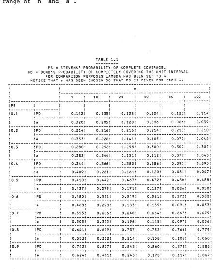
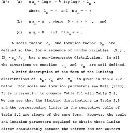
Table 1.1 below gives the two probabilities for a large range of n and a .

TABLE 1.1

PS = STEVENS’ PROBABILITY OF COMPLETE COVERAGE.

PD = DCMB'S PROBABILITY OF COMPLETELY COVERING THE UNIT INTERVAL FOR COMPARISON PURPOSES LAMBDA HAS BEEN SET TO n.

NOTICE THAT a HAS BEEN CHOSEN SO THAT PS IS FIXED FOR EACH n.

t t n

1 f _{5 ! 10 ! 20 ! 30 !} 50 ! 100 !

I_____

! PS

t — _

I J t t f I t t | » f

! 0.1 ! PD I 0.142 ! 0.135 ! 0.128! o »-* ro 0.120! 0.114 !

| t____

t _{! a} » _{0.320! 0.205 ! 0.128! 0.096! 0.066!} 0.039!

♦ ___ __

! 0.2 ! PD 1 0.214! 0.216! 0.216! 0.214! 0.213 ! 0.210!

t f___

1 _{! a} t _{0.353! 0.226! 0.141! 0.105! 0.072 !} 0.042 !

! —____

! 0.3 ! PD t 0.280! 0.292! 0.298! 0.300! 0.302! 0.302 !

t » _ ___

1 _{! a} f _{0.382 ! 0.244 ! 0.151! 0.112! 0.077! 0.045 !}

1_____

! 0.4 ! PD t 0.344! 0.366! 0.380! 0.386 ! 0.391 ! 0.395 !

\ 1___

t ! a | 0.409! 0.261 ! 0.161! 0.120! 0.081 ! 0.047!

I_____

! 0.5 ! PD f 0.410! 0.442 ! 0.463! 0.472 ! 0.480! 0.438!

f___

| _{! a} f 0.437! 0.279! 0.171! 0.127! 0.086! 0.050!

t_____

! 0.6 ! PD t 0.480 ! 0.521! 0.549 ! 0.561 ! 0.572 ! 0.582 !

t )___

| _{! a} » _{0.468! 0.298! 0.183! 0.135 ! 0.091 ! 0.053 !}

t___ —

! 0.7 ! PD I 0.555 ! 0.606! 0.640! 0.654! 0.667! 0.679!

t t___

1 _{! a} f _{0.505 ! 0.322 ! 0.196! 0.145! 0.097! 0.056 !}

1___ --- + _ --- + _

! 0.8 ! PD » 0.641 ! 0.699 ! 0.737! 0.752! 0.766! 0.779!

t 1___

I _{! a} | _{0.553! 0.352 ! 0.214! 0.158! 0.106! 0.060!}

f __

-! 0.9 ! PD t 0.742 ! 0.807! 0.845! 0.860! 0.872 ! 0.383 !

t t___ +

1 4.

It is clear from the values shown in Table 1 that Domb's probability is larger than Stevens' when Stevens' probability is large, and vice-versa when Stevens'

probability is small. Also when n is large there is not much difference between the two probabilities.

Stevens' and Domb's contributions constitute two

important but contrasting approaches to finding probabilities of complete coverage. One contribution may be more suitable than the other in some practical situations. For example, it may be more realistic to have a random number of intervals intersecting A . In this case Domb's work would apply.

In other situations, n {or N) may be very large, and a small. In this case an approximation to Steven's probability of complete coverage can be obtained. The

main issue here is how to define a limit theoretic approach because in reality both n and a are fixed. We can, however, view the observed event as a realization from a

sequence of coverage processes, indexed by n . That is, the n 'th coverage process consists of n arcs of angular radius a^ placed at random on the perimeter of a circle of circumference one. Notice that there is no constraint upon members of the sequence, such as mutual independence.

In the situation described above, let the vacancy,

, be the proportion of the perimeter remaining uncovered. Complete coverage of A occurs if and only if Vr = 0 ,

while the probability of complete coverage is P(Vn = 0) • Suppose that for each n we fix P(V = 0 ) = y , where 0 < y < 1 . Then a^ is determined by y .

Theorem 1.1 (Siegel (1979))

Let 3 = logd/y) . Then

a = r- log (§) + o (i)

n n p n

as n -* 00 .

Conversely, for fixed n and a^ we may invert

this result to obtain a first order approximation for y . The approximation is :

(1.6) y = P(V=0) = exp ( - n e na) ,

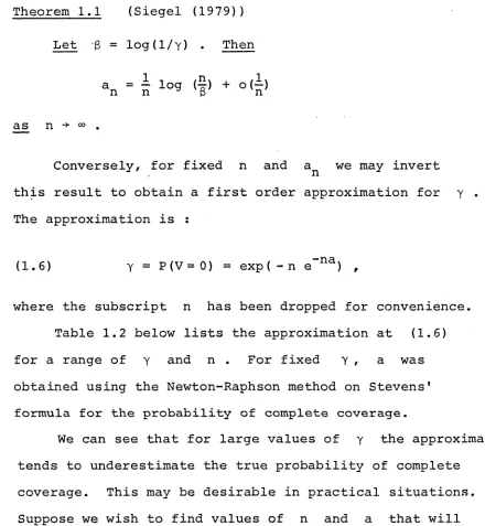
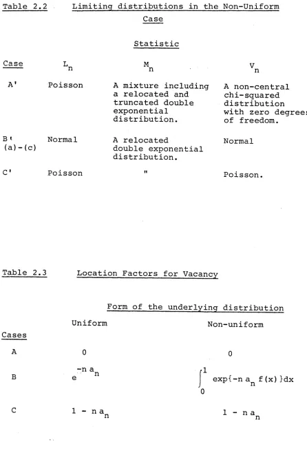
where the subscript n has been dropped for convenience. Table 1.2 below lists the approximation at (1.6) for a range of y and n . For fixed y , a was obtained using the Newton-Raphson method on Stevens' formula for the probability of complete coverage.

We can see that for large values of y the approximation tends to underestimate the true probability of complete

coverage. This may be desirable in practical situations. Suppose we wish to find values of n and a that will give us a large probability of complete coverage, y q say. Using Siegel’s approximation will ensure that P(V=0) > y q . In this respect the approximation may be considered as

conservative. In other situations we may want to ensure that the probability of complete coverage is smaller than a given small positive constant. Again, Siegel's

approximation leads to a conservative result.

16

TABLE 1.2

PS = STEVENS' PROBABILITY OF COMPLETE COVERAGE PSL = SIEGEL'S APPROXIMATION

» t _n f

1 t _{5 ! 10 ! 20 ! 30 ! 50 ! 100 !}

1_____________

! PS 1_____________ f --- +----1 1 J 1 1 J J 1 t t 1 1 t

! 0.1 ! PSL I 0.365! 0.277! 0.214! 0.187! 0.162! 0.139!

t f__________

1 _{! a} 1 _{0.320! 0.205 ! 0.128! 0.096! 0.066 !} 0.039 !

t_____

!0.2 ! PSL 1 0.426! 0.353! 0.300! 0.277! 0.255 ! 0.234 !

1 »_ _ _ ---+ -- ---+

-I ! a I 0.353! 0.226! 0.141! 0.105! 0.072! 0.042 !

1_____________ ---+

--! 0.3 ! PSL 1 0.476 ! 0.417! 0.376! 0.358! 0.341! 0.325 !

1 t - ________

I _{! a} t _{0.382! 0.244! 0.151! 0.112! 0.077! 0.045 !}

1 _____________

! 0.4 ! PSL J 0.523! 0.479! 0.448! 0.436! 0.424! 0.414!

t » __________ +

-1 _{! a} 1 _{0.409 ! 0.261! 0.161! 0.120! 0.081! 0.047!}

|

---! 0.5 ! PSL t 0.570 ! 0.540! 0.521! 0.514! 0.508 ! 0.503!

I 1 _ ___ +

-1 _{! a} t _{0.437! 0.279 ! 0.171! 0.127! 0.086! 0.050!}

1 _____________ ---+ --- +

-! 0.6 ! PSL » 0.618! 0.602! 0.595 ! 0.594! 0.593! 0.594 !

1 1 __________

1 _{! a} 1 _{0.463! 0.298! 0}

.183! 0.135 ! 0.091 ! 0.053!

1 _____________ --- +

»0.7 ! PSL I _{0.670 ! 0.670! 0.674! 0.678! 0.682 ! 0.687!}

1 t __________ --- + - .

1 ! a t 0.505! 0.322! 0.196! 0.145! 0.097! 0.056!

1 _____________

!0.8 ! PSL t _{0.730! 0.744! 0.759! 0.767! 0.775! 0.734!}

I 1 _______

1 _{! a} » _{0.553! 0.352 ! 0.214 ! 0.158! 0.106! 0.060!}

t _____________ --- + - --- + - +

-! 0.9 ! PSL J _{0.802 ! 0.833! 0.857! 0.867! 0.876! 0.885 !}

I I _______ +

-1 ! a 1 0.624! 0.401! 0.243! 0.178! 0.119! 0.067!

In recent literature on the subject of probabilities of complete coverage, several authors have attempted to extend the results of Stevens (1939) to the case of random arc lengths.

Siegel and Holst (1982) considered the following model. Suppose n arcs are uniformly and independently distributed on a circle A , of circumference one. The arc lengths

are assumed to be independently drawn from a distribution F on [0,1] . Furthermore, assume that the arc lengths and the distribution controlling the arcs' locations are independent.

We can see that this model contains Stevens' as a special case. Just allow F to be the step function :

0 when x < a , and (1.7) F (x) =

1 when x > a ,

where a e [0,1) . In other words, each random arc is of length a with probability one.

L e t 1 < k < n

'

Sk

-= 1 a n d ,

^k = ( k - 1 )! ■

„k

I . -I u i =l

u. „ V

k k j n-K

^i=l F(v)dv} du

1}

Siegel and Holst have shown that the probability of complete coverage is :

Pr(A is completely covered)

= £ (-1)k (?) 5k •

1 8.

This simplifies to Stevens' result (1.1) when F is the step function given at (1.7) . Following Stevens, Siegel and Holst obtained the probability of exactly m gaps occurring on the circle's perimeter. Indeed, if

0 < m < n ,

P(exactly gaps)

0 ? 0 < - n k"m

Of course, m=0 if and only if the circle is completely covered. Let us unwrap the circle onto the interval [0,1). Jewell and Romano (1982) have generalized the results of Siegel and Holst, on the probability of complete coverage, to a situation where the midpoint x and length £ of each arc follow a bivariate distribution, F , on [0,1) x [0,1) , which is continuous in x .

It is assumed that the n arcs are independently drawn from F . However, we do not require that the length and location of an arc be independent. Jewell and Romano

obtained the required probability by showing that the event of complete coverage is equivalent to the event that a random convex hull of n independent points from a bivariate

distribution G , determined by F , contains a disc.

The convex hull of a sample of size n is the smallest-area convex set containing all n points. Necessarily the set is the interior of a convex polygon. The vertices of

Suppose that Z = h w i t h p r o b a b i l i t y one, so that

each arc is a semicircle. Then, c o mplete cove r a g e is

d e t e r m i n e d by the l o cation of m i d p o i n t s a round the circle.

Let 0 be the c entre of the circle. If all n m i d p o i n t s

lie on one side of a line p a s s i n g through 0 , then the

circle is not c o m p l e t e l y covered. Conversely, if the

circle is not c o m p l e t e l y covered, then there is a line

pass i n g through 0 w i t h all m i d p o i n t s on one side of it.

Clearly, in this situation, the convex hull of the n

m i d p o i n t s does not c o n tain 0 . Therefore, the c ircle is

c o m p l e t e l y co v e r e d if and only if the convex hull of the

n m i d p o i n t s c o n t a i n s 0 . W i t h o u t too m u c h difficulty,

it m a y be shown that the p r o b a b i l i t y of this event is :

P = 1 n [ {F (u) + 1 - F (u + h) )n-1 du

(F(u) F (u - h) l11” 1 du ] ,

w h e r e F(u) = F : „ , ‘x=u, Z = h .

In general, however, Je w a l l and Romano have o b t a i n e d

formulae for the p r o b a b i l i t y of c omplete cove r a g e of the

circle. The s o lution is not given here as its form is

2 0.

§1.2 The Higher Dimensional Case

We shall call the coverage set A k-dimensional if there exists a one-to-one topological transformation, T , such that T(A.) has non-zero content in k-dimensional space. It is possible for A to be a subset of a higher dimensional space. For example, the perimeter of a circle of circumference one is a subset of HR2 . However, by unwrapping the perimeter we may map the circumference into a subset of IE*} . Therefore, Stevens' (1939) problem is one-dimensional. In this project we shall never explicitly state the form of T because in most cases the

dimensionality will be obvious.

A coverage process consists of randomly placed sets on A . As in the one-dimensional case, A is completely

covered if it is contained in the union of the random sets. To see why probabilities of complete coverage are often more difficult to find in the higher dimensional case,

consider the following argument. Take a 1-dimensional section through A . If A is covered then so is any section.

However, in order that A is completely covered we require that all sections through A be completely covered. There are uncountably many such sections and even though it may be possible to find the probability that any one is covered, it would be much more difficult to find the probability

the exact probability that n randomly placed hemispheres covered a sphere.

Two early authors to obtain significant results in higher dimensional coverage problem were Moran and

Fazekas de St Groth (1962) . Suppose n points are

independently and uniformly distributed on the surface of a sphere. On the surface of the sphere are placed n circular caps, each subtending an angle 2a , their poles coinciding with the random points. Moran and Fazekas de St Groth used this model to solve a problem which arises in virology.

Suppose an approximately spherical virus enters an organism. Cigar shaped antibodies attach themselves end-on to the virus. Each antibody prevents a circular cap area on the surface of the virus from attacking the host's cells If enough antibodies are spread over the virus then it will be impossible for the virus to infect any cell. This

situation corresponds to complete coverage of the sphere by circular caps, each of angular radius a = 53° . We shall again refer to this interesting application of coverage in section 4 . In the following paragraphs we outline the heuristic method used by Moran and Fazekas de St Groth to find the probability of complete coverage.

- 1/2

Suppose the sphere has radius ( 4tt) and surface area 1 . The vacancy V is the surface area of the

uncovered portion of the sphere. Let P = P(V=0) .

When V = 0 we say that the sphere is completely covered. The distribution of V , given V > 0 , is continuous with first and second moments \i1 and y 2 #■ say. The

2 2.

be shown to be

M 2 { E (V ) } 2

1 - P = --- . Hi E ( V 2 )

It is p o s s i b l e to de r i v e closed f orm e x p r e s s i o n s for the

first two m o m e n t s of vacancy. In section 2 we d i s cuss a

general m e t h o d of finding m o m e n t s of v a c a n c y d e v e l o p e d by

Robbins (1945) . M o r a n and F a z e k a s de St Gro t h showed that

E (V) = (1 - a) n

and

E ( V 2 )= _% (* TT

{1 - f (cj>) } sin (4)) d<J> /

w h e r e a is the area of a c i r c u l a r cap, and f($) is

the area of the union of two c i r c u l a r caps separated by

angle <fi . The m o m e n t s of the c o n t i n u o u s part of V

are found in the fol l o w i n g way.

W h e n a is small n will be large b e fore c omplete

c o v e r a g e occurs. If the sphere is alm o s t co m p l e t e l y

covered, then there will be a n u m b e r of small u n c o v e r e d

regions. The areas of the u n c o v e r e d regions will be

a p p r o x i m a t e l y i n d e p e n d e n t * r a n d o m variables. Furthermore,

it is not u n r e a s o n a b l e to as s u m e that their nu m b e r has an

a p p r o x i m a t e P o i s s o n distribution.

Since the u n c o v e r e d regions are small, their p e r i m e t e r s

will c o n s i s t of a l m o s t s t raight lines. The p e r i m e t e r of a

given region can be m o d e l l e d by a r a n d o m n e t w o r k of lines

in the plane. This r a n d o m line n e t w o r k is a special case

of a P o i sson plane process. See, for example, Mil e s (1970

a,b, 1971 and 1972) . We shall d i s c u s s Miles' w o r k in

Fazekas de St Groth were able to utilize results on the expectation and variance of the area of regions generated by random line networks to obtain approximations for yi and y 2 t and hence P .

In the virus example discussed above, this approach led to the following approximation to the probability of complete coverage :

The analytic techniques used by Moran and Fazekas de St Groth differ greatly from the methods employed in the one-dimensional case. For example, the possibility of ordering the intervals in the one-dimensional case allowed Stevens to obtain a simple formula for the exact probability of complete coverage. There is no simple way of ordering

sets in higher dimensional problems.

Perhaps the major concern with Moran and Fazekas de St Groth1s work is the heuristic nature of some of their proofs. To a great extent Gilbert (1965) overcame these problems. He also realized that an exact expression for the probability of completely covering a sphere could be obtained when a = 90° .

When a = 90° the spherical caps become hemispheres. Using an argument similar to Gilbert's we shall prove

that the probability of complete coverage is I T2

P ~ exp{- (2 E V (1 + 0.025666 2))

(1.8) 1 - (n2 - n + 2 ) 2

In an earlier work Wendel (1962) showed that if n points are randomly scatter ed on the surface of a unit

2 4 .

all the points lie in some hemisphere is :

k-1

-(1.9) 2 n 1 Z (n_1) .

j=0 3

The n hemispheres will be randomly and uniformly located on the surface of the sphere if the poles of the hemisphere are located at independent, uniformly distributed points. We shall show that the events : n points lying inside some hemisphere, and the sphere is not completely covered are the same. It will follow that the probability of complete coverage is given by (1.9) .

Without loss of generality assume that the spheres is centered at the origin 0 . Suppose the n points lie inside a hemisphere with pole z . Then the point -g , also on the surface of the sphere, is not covered.

Conversely, if there exists a point z which is not

covered, then the hemisphere with pole at -z covers all n points. Therefore, the two events are the same.

In three dimensions k=3 and (1.9) specializes down to

(1 .8 ) . |“ |

A crossing is defined to be the intersection of the boundaries of two caps. The crossing is said to be covered if any random cap, excluding the two which define it, contain the crossing. Let G(n) be the expected number of uncovered crossings and U(n) the expected number of uncovered crossings when not all crossings are covered.

U (n) = (1 - P) G (n) . Hence

(1.10) P = 1 - {G(n)/U(n) } .

However, the usefulness of (1.10) lies in the fact that U(n) -*■ 4 as n . Gilbert proved this for a = 90° . Miles (1969) later established this for all values of a satisfying 0 < a < 90° . The asymptotic

approximation derived from this result and expression (1.10) is

P ~ 1 “ n(n-1)a (1-a)n ^ .

So far we have only considered coverage probabilities for circular caps placed at random on the surface of a sphere. Miles obtained generalizations of Gilbert's

results for spherical polygons which are not only randomly located on the surface of a sphere, but are also randomly rotated according to a uniform distribution. This may be defined in strict terms as follows.

Let S be an arbitrary set on the surface of a sphere A . Suppose the surface area of A is 1 . A random

copy of S is made so that

(i) an arbitrary point in S goes to a point which is uniformly distributed on the sphere's surface, and independently of this

(ii) the orientation of S about this point is uniform.

26 .

the number of , 1 < i < n , which cover x ,

H = sup , H(x) and H = inf , H(x) . We may

interpret H and H as the number of coverings on the

least and most covered regions of the sphere's surface,

respectively. It is clear that the sphere is completely

covered if and only if H > 0 .

Miles generalized Gilbert's results in two different

ways. Firstly, as previously mentioned, he obtained

asymptotic approximations for the probability of complete

coverage for spherical polygonal shapes. Secondly, he

obtained approximations for P(H = m) and P(H = n-m)

for fixed values of m. Miles' result is set out in

Theorem 1.2 below.

Theorem 1.2 (Miles (1969))

Let the area of S be a , and its perimeter be b .

Then, as a+°° , both

P(H=m) and P(H<m) _{(m + 2 ) (m + 1 ) (m + 2 ) b 2}

m , - v n - m - 2 a (1-a)

4 TT

while both

P(H>n-m) and P(H=n-m)

(m + 2 ) (m+1)(m+2)b2

n -m-2 xm

a_______ (1-a)

4tt

where m > 0 .

Theorem 1.2 continues to hold for shapes which can be

approximated by spherical polygons. A circular cap is one

such shape.

As mentioned in subsection 1.1, it is possible to construct a coverage process on the unit interval rather

surface of a sphere. However, when the coverage region is rectangular, edge effect problems occur. Miles used a simple method which overcame edge effects. Essentially it converts the rectangle into a "topological torus" . Since the topological torus is of importance in the

theoretical section of this project we shall describe it in detail here.

Suppose the rectangle, A , has sides of lengths and Ü2 . Orientate A so that its left hand corner

is at the origin and its sides are parallel to the

co-ordinate axes. For simplicity, assume the basic shape S is bounded by a circle with radius no greater than min(£i,£2) • A random copy of S is defined so that

(i) an arbitrary point of S is at a uniform random point in A , and

(ii) the orientation of S about this point is uniform.

For illustrative purposes we shall only deal with one random copy of S . The generalization to n independent random copies shall be obvious.

Let be a random copy of S . Diagram 1.1 shows a typical for a non-spherical basic shape. Now, translate to eight different positions by moving it the width of A left and right, the height of A up and down and any other combination of these movements. Diagram

28 . Diagram 1.1:

Diagram 1.3

dimensions.

It is possible to extend the topological torus

technique to higher dimensional space. The method is very- similar to the two dimensional case described above, so we refer the interested reader to Gilbert's (1965) paper. Diagram 1.3 shows the effect of the torus topology on a

3 2.

In a k-dimensional rectangle, H and H may be defined in a similar way to before. Imposing a torus topology on the rectangle, Miles obtained results which described the asymptotic behaviour of P (H = m) and

P(H = n-m) as n tends to infinity. These results are in essence generalizations of the theory for the spherical case. (There are some minor complexities introduced in defining a uniform random rotation in greater than two

dimensions.) For the types of random covering shapes Miles considered, the following approximation to the probability of completely covering the rectangle was obtained :

where a is the content of S , b its surface area, and || A || is the content of A .

Let us now explore the ideas discussed by Moran and Fazekas de St Groth (1962) on the size and structure of the small vacant regions obtained when a sphere is almost

completely covered by random caps.

As Miles had done in his 1969 paper we can generalize the coverage problem into a k dimensional setting.

Suppose, however, the sequence of "random shapes" {S^} are now centred at the points of a Poisson process of uniform intensity, A , on ]R . (In Chapter 2 of this project we shall describe in a theoretical manner what is meant by the term "random shape".) The structure of the uncovered gaps can be approximated by convex regions formed by a Poisson field of (k-1)-dimensional planes in HR , which we now describe.

TT%2k { r (3s(k+l) ) }k-1

Let Ci / £2/... be points of a Poisson process on [0,°°) and 0 1,0 2/ ... be unit vectors uniformly and

independently distributed on the surface of the k-dimensional

unit sphere centred at 0 . Let be the k-1

dimensional plane whose normal to the origin has length and inclination 0^ . The Poisson field of k-1

dimensional planes in JR is formed by the planes tt^ , J^

i > 1 . The planes , i > 1 f partition JR into a sequence of convex polygons, each identically distributed.

Miles (1970 a,b, 1971 and 1972) has investigated in

detail Poisson plane processes, but in a more general context. The random planes, or flats as described by Miles, are

s-dimensional where 1 < s < k . A stochastic flat process of intensity y > 0 in JR is defined so that it is

stochastically invariant under any translation or rotation. Let X be an arbitrary (k-s)-dimensional subset in JR with (k-s)-dimensional content ||x|] . The stochastic process is such that the number of s-flats intersecting X has a Poisson distribution with mean

y j|

j

3 4 .

§2 Vacancy

In the previous section we spoke of the coverage region, A , as a fixed subset of k-dimensional space. The coverage process consists of randomly placing shapes upon A . Let us define an indicator function I as follows. For each x E ]R , let

1 if x is not covered by any random shaoe, and

I(x) =

0 otherwise.

The vacancy, or the content of the uncoverd region in A is

(2.1) I(x) dx

In all situations investigated in this project, the random shapes and A are always Lebesgue measurable subsets of 3R . Thus, if we interpret the right hand side of (2.1) as a Lebesgue integral and assume that the content of A is finite, then V is well defined as a random variable.

In some situations, it may be more convenient to investigate the properties of the Lebesgue measure of the covered region in A , defined by

C {1 - I (x )} dx . A

Suppose that A is completely covered by random shapes. Then I(x) = 0 for all x in A , and V = 0 . However, the converse is not true; for it is possible

that a set of Lebesgue measure zero could be left uncovered. Such problems do not occur frequently in practice because the probability of a zero measure set, except in

artificial examples, is zero.

A large amount of work on vacancy in stochastic coverage processes is concerned with either finding the moments of vacancy, the exact distribution of vacancy or

approximations to the distribution of vacancy through limit theoretic methods. Any particular research paper usually deals with more than one of these topics because the results in one area are quite likely to depend on the results in another. Thus, it was decided not to discuss each topic in a different subsection, but rather deal with the work in a chronological fashion. However, this will tend to

segregate the topics, as the early work is primarily concerned with moments and the exact distribution of vacancy, while more recent work has concentrated on the limit theoretic

approach. As was the case for probabilities of complete coverage, exact results for the distribution of vacancy are usually confined to the simplest geometrical models. The reasons for this are made clear by the following.

If the random process controlling the location of shapes in A is such that no two shapes can overlap, or no shape can intersect the boundary of A, then the vacancy is solely determined by the content of A and of

each shape. On the other hand, if the random shapes

3 6.

of shapes. Thus, in the one dimensional situation, vacancy can be described in terms of the starting position of each interval and their lengths. However, in the higher

dimensional situation there is the difficulty of arranging the random shapes in order, and hence of simply describing vacancy. Domb (1943) was one of the first authors to

attempt to find the exact distribution of vacancy in a one dimensional situation.

The coverage process he studied was described in subsection 1.2. We repeat the description here for convenience.

Intervals of length a are centred at the points of a Poisson process of uniform intensity A . Domb was interested in vacancy in the interval [0,y] . As

previously noted, it is sufficient to consider the coverage of the unit interval A = [0,1] .

Let F be the distribution function of the

covered portion, C , in A . Let x > 0 and [x] be the integer part of x . It is possible for A to contain r non-overlapping intervals none of which overlap the

endpoints of A , where r = 0,1,2, . ..,[1/a] . Therefore, F possesses discontinuities at r = o,a,2a,...,[i]a . Using a Dirac 6-function notation, Domb wrote down the Laplace transform of the "density of F" , which may be expanded to find an exact expression for F . Due to the complexity of the final result, he never did this. However, Domb

showed that the size of the r 'th discontinuity to be :

P(C = ra) = 2r (l-ra)r e“X(a+1)/r!

Even in the one d i m e n s i o n a l situation, studied by

Domb, exact e x p r e s s i o n s for the d i s t r i b u t i o n of v a c a n c y

are d i f f i c u l t to obtain. However, there is a simple

t e c h n i q u e a v a i l a b l e for finding the m o m e n t s of vacancy,

w h i c h e asily g e n e r a l i z e s to the hi g h e r d i m e n s i o n a l case.

R o b bins (1944) e x p r e s s e d the p r o b l e m in terms of the m o m e n t s

of the m e a s u r e of a r a n d o m set.

L e t ft be the set of all p o s s i b l e L e b e s g u e

m e a s u r a b l e subset of IR . A p r o b a b i l i t y d i s t r i b u t i o n

of r a n d o m sets, 6 , is d e f i n e d so that the p r o b a b i l i t y

that x E ft b e l o n g s to a 6-measu r a b l e subset, S , of

ft is :

P r

(x e s)

'ft s

w h e r e y is the c h a r a c t e r i s t i c function of S .

‘S

Let y be L e b e s g u e m e a s u r e in 3R . The m e a s u r e

of X m a y be r e - w r i t t e n as :

(2.2) y (X) Iv (x) dy(x) , 'ft X

whe r e

1 if x E X , and

V x)

-0 if x € X .

Ta k i n g the e x p e c t a t i o n inside the integral on the right

h and side of (2.2) gives

E{y(X) } E{ Ix (x) } dy (x)

as the expected measure of X . Using a similar method it is possible to show that

3 8.

(2.3) E { y ™ ( X ) } ' P(xn E X, x n E X,...,x E X) dy(x..) ...

1 2 m 1

ay (x^)

where m > 1 . We may easily apply Robbins' results

to vacancy; for vacancy is just the measure of the random

uncovered region in A . Robbins applied his results to

find the expectation and variance of vacancy in an interval

[0,y] covered by n randomly and uniformly located

intervals of length a . To overcome edge effects he

extended the distribution controlling the location of

intervals beyond the endpoints of [0,y] . Bronowski and

Neyman (1945) used a similar method to overcome edge effects

in a related two dimensional set-up.

Let N be a non-negative integer-valued random

variable with probability generating function <p , defined

by :

co n

(Ms) = Zn=0 s P (N=n) .

Suppose that the coverage region, A , is rectangular

with side lengths b and c . Now N points are uniformly

and independently distributed in a concentric rectangle,

A' , of side lengths b+2y , and c+2y , where y > 0 .

Let rectangles of side lengths a and 3 , where a <2 y

and 3 <2 y , be centered at the random points. Each random

rectangle is oreinted in the same direction so that their

sides are parallel to those of A . Finally, write a = a3

makes it possible for a random rectangle to not intersect A . See diagram 2.1 below. In this sense the edges of A' do not affect the coverage of A . This is sufficient

to remove edge effects from the problem.

Under the above conditions, Bronowski and Neyman showed that the first moment of vacancy in A is :

(2.4) E (V) = || A|| (Ml - a/ ||A'|| )

and a much more complex expression holds for the variance of V. Expression (2.4) includes the cases where the centres are distributed according to a Poisson process in A' , and

40

Diagram 2.1 :

A rectangle centred close to the boundary of A' does not intersect A.

$

I

I

l

I

I

I I I I

The method of finding the moments of vacancy used by Bronowski and Neyman differs from the general methods of finding moments of the measure of a random set

suggested by Robbins (1944). Bronowski and Neyman

considered vacancy on a sequence of lattice points which, if made sufficiently fine, approximated vacancy, and hence expected vacancy, in the region of A . However, as was previously shown by Robbins, the moments of vacancy can be obtained through the integral expression (2.3) .

In a subsequent paper, Robbins (1945) used the methods he developed in 1944 to generalize the results of Bronowski and Neyman to a k-dimensional situation. Essentially, N k-dimensional shapes are independently

and uniformly distributed over a region, A' , which contains the rectangular coverage reion, A . Each random rectangle is oriented in the same direction so that their sides are parallel to the sides of A . The region A ’ is suitably chosen to remove edge effect problems. Again, a probability generating function is introduced for N .

In the abovedescribed situation, Robbins obtained expressions for mean and variance of vacancy, which- involved considerably less technical derivations than used by

Bronowski and Neyman.

Robbins also found expressions for the mean and variance of vacancy when N circles of area a were independently and uniformly distributed on A .

For rectangular shapes the expression for variance depends on the area of the intersection of two shapes whose centres are separated by a vector x . However, for

4 2.

the distance that separates the two centres, r = |x| , say. Thus, the variance expression for circular shapes is somewhat simpler than for rectangular shapes, and, indeed, for more general random covering shapes. In the later sections of this project we shall develop formulae for the variance of vacancy in a very general framework.

The work of Bronowski and Neyman (1945) and

Robbins (1944, 1945) suggests that formulae for expectation and variance can be obtained for a more general class of shapes, which have been distributed at random throughout a given region, A' . Garwood (1947) proved this to be the case for any shape S bounded by a simple closed curve.

The context in which the theory was developed, was in application to a bombing problem. The area destroyed by a single bomb is represented by a circular region of radius r on the ground. A building is represented by a

rectangular region A . The amount of the building destroyed by a cluster of bombs is just the area in A covered by

n randomly positioned circles. We shall discuss this application in greater detail in section 4 of the present chapter.

Garwood investigated vacancy for a variety of covering shapes and regions. We shall, however, describe the general coverage process in which each special case can be represented. Let A be the interior of a simple closed curve and S the

and N a n o n - n e g a t i v e i n t e g e r - v a l u e d ra n d o m v a r i a b l e

i n d e p e n d e n t of (X,0) . A r a n d o m copy of S is o b t a i n e d

by r o t a t i n g S through 0 abo u t c and then t r a n s l a t i n g

the n e w set through X . Let ^ i ' ^ 2 ' aaa a seciu e n c e °f

i n d e p e n d e n t r a n d o m copies of S . The c o v e r a g e p r o c e s s is

f ormed by the r a n d o m shapes S ^ , ...,S^ , and w e are

i n t e r e s t e d in the v a c a n c y V in A .

A c c o r d i n g to Robbins (1944) , to o btain the first

m o m e n t of v a c a n c y we require the p r o b a b i l i t y that x G A

is not c o v e r e d by a single r a n d o m shape. Let S(v,0) be

the set S c e n t r e d at y and rotated through 180° + 6 .

C o n d i t i o n a l on it being i nclined at 0 , does not

cover x if its centre does not fall in the region

A ' \ S(x,0) . Therefore, the p r o b a b i l i t y that does

not cover x is :

If N has p r o b a b i l i t y g e n e r a t i n g f u nction <J> , the

p r o b a b i l i t y that x b e l ongs to the v a c a n t region in A

is 4> (p (x ) ) . Therefore, the e xpected v a c a n c y is

G a r w o o d also o b t a i n e d the f o l l owing formula for the

second m o m e n t of v a c a n c y using an a r g u m e n t similar to

that above :

p(x) =

0 A ’\ S ( x , 0)

f ( x ,0)dx d 0 .

E (V) = <J>{p (x) ) dx

J

A

E (V2 ) = 4>(p(x,y)} dx dy