Cell lineage visualisation

This is a repository copy of Cell lineage visualisation.

White Rose Research Online URL for this paper:

http://eprints.whiterose.ac.uk/84341/

Version: Accepted Version

Article:

Pretorius, AJ, Khan, IA and Errington, RJ (2015) Cell lineage visualisation. Computer

Graphics Forum, 34 (3). 21 - 30. ISSN 0167-7055

https://doi.org/10.1111/cgf.12614

[email protected]

Reuse

Unless indicated otherwise, fulltext items are protected by copyright with all rights reserved. The copyright

exception in section 29 of the Copyright, Designs and Patents Act 1988 allows the making of a single copy

solely for the purpose of non-commercial research or private study within the limits of fair dealing. The

publisher or other rights-holder may allow further reproduction and re-use of this version - refer to the White

Rose Research Online record for this item. Where records identify the publisher as the copyright holder,

users can verify any specific terms of use on the publisher’s website.

Takedown

If you consider content in White Rose Research Online to be in breach of UK law, please notify us by

Eurographics Conference on Visualization (EuroVis) 2015 H. Carr, K.-L. Ma, and G. Santucci

(Guest Editors)

Volume 34(2015),Number 3

Cell lineage visualisation

A. J. Pretorius1, I. A. Khan2, and R. J. Errington2

1_{School of Computing, University of Leeds, UK} 2_{School of Medicine, Cardiff University, UK}

Abstract

Cell lineages describe the developmental history of cell populations and are produced by combining time-lapse imaging and image processing. Biomedical researchers study cell lineages to understand fundamental processes, such as cell differentiation and the pharmacodynamic action of anticancer agents. Yet, the interpretation of cell lineages is hindered by their complexity and insufficient capacity for visual analysis. We present a novel approach for interactive visualisation of cell lineages. Based on an understanding of cellular biology and live-cell imaging methodology, we identify three requirements: multimodality (cell lineages combine spatial, temporal, and other properties), symmetry (related to lineage branching structure), and synchrony (related to temporal alignment of cellular events). We address these by combining visual summaries of the spatiotemporal behaviour of an arbitrary number of lineages, including variation from average behaviour, with node-link representations that emphasise the presence or absence of symmetry and synchrony. We illustrate the merit of our approach by presenting a real-world case study where the cytotoxic action of the anticancer drug topotecan was determined.

Categories and Subject Descriptors(according to ACM CCS): I.3.8 [Computer Graphics]: Applications— J.3 [Com-puter Applications]: Life and medical sciences—Biology and genetics

1. Introduction

Biology is in the midst of a paradigm shift. In contrast to small-scale bench-top experiments, high-throughput mi-croscopy enables biologists to design and automate large-scale screens and collect results as digital images [Jen13]. Time-lapse microscopy captures the dynamic behaviour of live samples by acquiring images at regular intervals and image processing algorithms then track objects across con-secutive images. The most sophisticated approaches produce cell lineages by combining tracking with event detection, where key cellular events such as cell division (mitosis) and cell death are identified [ECKe13]. Image processing algo-rithms also derive descriptive measures, including properties related to location, morphology, and motility [CJLe06].

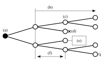
Cell lineages describe the genealogy of populations of cells, capture information on cellular development, and rep-resent contiguous cell cycles [Kha08,GLHR09]. A cell lin-eage is a tree structure where vertices depict cells and edges depict descendant relationships (see Figure 1). The root represents the progenitor (the cell originally tracked; Figure 1(a)) and descendent nodes represent the progeny (generations of offspring; Figure1(b)). A lineage captures key events such as cell division and cell death (Figure1(c)

and (d)) and additional data are often associated with nodes (Figure1(e)). This includes spatial locations of events, tem-poral data, and derived properties. Temtem-poral intervals be-tween events capture cell cycle parameters. Every level cor-responds to a generation of cells (Figure1(f)) and non-death leaves correspond to the end of an experiment (Figure1(g)). Despite the proven value and popularity of live-cell imag-ing [Car07], it is difficult to extract insights from time-lapse experiments [WSBe10]. To address this, we present a novel interactive visualisation method for cell lineage data.

2. Related work

Several visualisation methods have been used to analyse data derived from live-cell imaging. We survey these below.

2.1. Image-based approaches

(a)

(b) (c)

(d) (e)

(f) _(g)

Figure 1:A cell lineage captures how (a) a progenitor cell proliferates into (b) a progeny, or population of offspring. It describes key cellular events such as (c) cell division and (d) cell death. (e) Additional data are often associated with cells. (f) Every level corresponds to a generation of cells and (g) non-death leaves correspond to the end of an experiment.

time to the x-axis and imaging modalities to the y-axis, it has been used to study the effect of viral infections on cell motility [HLLK09]. A related method shows the temporal changes of associated measures as a heatmap superimposed on images. It has enabled scientists to analyse relationships between cell division and protein localisation [GBBS09].

Visualisation of image data is useful for small-scale ex-periments and for reporting. These methods, in particular movies, illustrate the dynamic nature of the data. Still, due to inherent scalability limits, analysis of larger experiments is challenging. It is also difficult to make comparisons within and across experiments to draw higher-level conclusions.

2.2. Aggregate plots

A popular way to address scalability is to derive measures from image data and to visualise these at a cell population level. Examples include [JKWe08]: histograms to show dis-tributions of cells by, for example, their DNA content; scat-terplots to consider relationships between pairs of derived measures, for example, overall cell area versus cell nucleus area; parallel coordinate plots to consider an arbitrary num-ber of measures; and density plots where, for a pair of mea-sures, the number of data points that map to a particular co-ordinate are colour-coded.

Aggregate plots are useful for scenarios such as gating: the identification of thresholds for perturbations, such as drug dosage, to affect cell phenotypes [JKWe08]. These “hits” are important for drug discovery. Because the plots are familiar to many users, they are also effective for reporting purposes. However, it is difficult to analyse low-level data, such as single cell behaviour. Time, which is an important property of time-lapse data, is also not treated explicitly.

2.3. Temporal plots

Temporal plots map aggregate data to a time axis. For exam-ple, plotting the population size of a cell simulation model

as a function of time reveals different phases of development in the resulting line chart [GLHR09]. A similar approach, where structural properties of cell colonies cultivated under different conditions are mapped to time, highlights different behavioural dynamics for each condition [SHTe12].

In such aggregate representations, it is hard to deter-mine if similar behaviour is exhibited across the board. This can be addressed by aligning temporal plots by signif-icant occurrences, such as a sudden drop in a derived mea-sure [SMCe06]. Another approach is to consider key cellu-lar events. Cumulative event curves, where running totals of event types are mapped to time are useful for contrasting experimental conditions, such as drug treatment, to control conditions [KHCe07]. Typical event sequences can also be derived from time-lapse data. Event-order maps show these and allow event-based behaviour corresponding to different experimental conditions to be characterised [WHNe09].

Users relate well to time. However, temporal plots typi-cally show aggregate behaviour and do not support analysis of individual cells and relationships between them.

2.4. Space-time cubes

Space-time cubes, adopted from time geography [Häg70], are a mainstay of time-lapse data analysis. Cellular trajecto-ries are mapped to space (x- and y-axes) and time (z-axis) in 3D. This gives rise to problems like overplotting and occlu-sion [War01], and requires data filtering and navigating to an appropriate perspective, which is cumbersome. Despite their popularity, it is hard to find an example of real insight ob-tained from space-time cubes in a live-cell imaging context.

2.5. Dimension reduction

Images can be considered as vectors of features that describe quantified properties of cells or statistical properties of the images themselves [HWKT09]. Dimension reduction tech-niques, such as principal component analysis and Sammon mapping, are then used to project images to 2D so they are near each other when their descriptive vectors are proximate in high-dimensional space [Fod02]. This is useful for sug-gesting correlations and similarity classes. Still, since the semantics of the high-dimensional distances that these meth-ods preserve are usually unclear, it is challenging for users to relate visual patterns to data characteristics.

2.6. Cell lineage visualisation

A. J. Pretorius, I. A. Khan, & R. J. Errington / Cell lineage visualisation 3

cells [GLHR09,KHCe07]. Although node-link diagrams are effective for showing structural properties, implementations are typically very basic and do not support in-depth analysis such as comparisons between multiple lineages. Also, lin-eages cannot be considered in the context of associated data such as spatial location and experiment parameters.

Stream-like visualisations have been used to show the temporal behaviour of entire cell colonies [SHTe12]. How-ever, this approach does not enable analysis of individual lineages in the context of larger populations of cells.

2.7. Tree visualisation and movement data

Many methods exist to visualise single [Sch11], and mul-tiple trees [GK10]. Advanced approaches allow structural comparisons of arbitrary numbers of trees, but unlike cell lineages, they require trees to either have identical leaves [BvLHe11], or to have predefined meaning associated with structural properties [LKBe14]. These methods were not developed to emphasise the aspects highlighted by our requirements analysis (see next section). As we will show, for individual lineages, domain experts have a clear prefer-ence for directed node-link views (subject to our require-ments). This rules out other tree visualisation methods.

We also reviewed visualisation methods for movement data [AA13]. In contrast to cell lineages, they cater for object trajectories that do not divide, usually in geographic space.

3. Requirements analysis

All the above methods have drawbacks that limit their suit-ability for rigorous cell lineage analysis. To better under-stand the requirements for cell lineage visualisation, we con-sidered biologists’ objectives and analysis paradigm, the bi-ological phenomena described by lineages, and their data characteristics. For this, we consulted biomedical domain experts (second and third author) and reviewed the litera-ture on high-throughput microscopy. Further domain experts were involved during a two-day workshop.

3.1. Multimodality

Cell lineages combine relational, spatial, and temporal data. Further, a key characteristic of high-throughput analysis is the processing of image data to generate additional derived properties for individual cells. This produces multivariate data that are associated with cell lineages, including cell cycle phases and event types [GLHR09]. Finally, metadata describe different experimental conditions, such as adminis-tered drugs and their concentrations. Downstream process-ing may generate more metadata, for example, to classify collections of lineages. There is an unmet requirement to support visual analysis of the multimodal data associated with cell lineages at different levels of detail, from different perspectives, and across multiple data sets.

3.2. Symmetry

Biological studies have shown that cells and their descen-dants often escape from perturbation effects. There is evi-dence that drug delivery to progenitor cells is heterogenous due to underlying drug-resistance properties [CECe08], and that the consequences of drugs are distributed asymmetri-cally in the progeny of tumour cells [SMKM10]. This sug-gests that, when viewed with respect to branching points, subtrees in a cell lineage structure will differ. The prolifera-tion of cells represented by some subtrees will be adversely effected while other subtrees will appear to remain unper-turbed. Users must be supported in studying the presence or absence of lineage symmetry in terms of cellular events (cell division and cell death), but also in terms of additional derived properties. This requirement is not met by the visu-alisation techniques available to biomedical researchers.

3.3. Synchrony

The cell cycles of healthy and unperturbed cells are expected to exhibit conserved and regular temporal behaviour across generations [KLCe11]. For example, apart from stochastic variation, healthy cells generally have approximately equal inter mitotic times as a population of cells proliferates. In contrast, perturbed cells such as those in tumours or those treated with drugs, are expected to exhibit more heteroge-neous temporal behaviour. This implies that an emphasis on temporal responses and timing of events, especially their degree of synchronisation across generations, is important. There is an unmet requirement for interactive visualisation techniques that support users in analysing cell lineages to identify and investigate the causes of temporal asynchrony and how it relates to cellular events and the cell cycle.

4. Design

Section3shows that a critical gap remains: there is currently very limited visualisation support to fully exploit cell lineage data for hypothesis-driven or explorative analysis. To bridge this gap, we developed a novel approach for cell lineage vi-sualisation. Over a period of 18 months we combined the expertise of a visualisation designer (first author), a bioin-formatician (second author), and a cell biologist (third au-thor). We followed an iterative design process by meeting bi-weekly [PvW09]. The designer demonstrated progress on a software prototype, while the biologists provided feedback grounded in domain knowledge. Other domain experts pro-vided input during a workshop.

sym-0 0.5 0

1.5 2 0.5 0.5 1.5

1

(b)

1 2 3.5 1

(c)

Gen.0 Gen.1 Gen.2 Gen.3

Lin.A Lin.B Lin.C

M1 M2 M3 1 2 1 a a b α β γ M1 Lin.A Lin.C 1 Lin.B 2 M2 Lin.A Lin.B a Lin.C b M3

Lin.A Lin.B Lin.C

α β γ

(a)

Lin.C

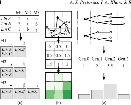
Figure 2:(a) Grouping by metadata values. Lineages A, B, and C are grouped according to the different values they take for metadata fields M1, M2, and M3. (b) Spatial summaries of groups of lineages. The field of view is divided into dis-crete regions (3×3 in this example), and the average num-ber of events per region is visualised as a heat map. (c) Tem-poral summaries of groups of lineages. The average number of events per generation is visualised as a bar chart.

metry and synchrony requirements are addressed by a repre-sentation that emphasises these properties (Section4.3).

4.1. Spatiotemporal overview

We designed an overview to show the dynamics of poten-tially large numbers of lineages. In this section, we describe how we enable users to aggregate lineages into groups and how the spatial and temporal behaviour of groups of lineages are visualised.

Grouping.For every lineage, metadata fields describe ex-perimental parameters such as drug treatment and drug dosage. Metadata are usually categorical, take a small num-ber of values (≤20), and users understand their meaning. We

therefore apply the principle of faceting to show lineages in terms of metadata [Tun09]. As Figure2(a) shows, for ev-ery user-selected metadata field, lineages are grouped by the value they take for that field. Every group is shown as a rect-angular icon that combines a summary visualisation of the spatial and temporal behaviour of its member lineages.

Spatial summaries.The locations of cellular events are an important analytical grounding for users and the top of ev-ery icon summarises the positions of events in the field of observation. Figure2(b) illustrates our approach. We divide the field into rectangular regions and, for all lineages in a group, show the average (mean) number of events that oc-cur in every region with a heatmap. Averages are binned and colour-coded using an ordinal colour map [Bre]. The number of regions is parameterised, but we find a small number, cur-rently 5×5, sufficient for aggregate behaviour (Figure3(a)).

We considered several design alternatives. Initially, we showed the smallest convex polygon that contains all lin-eage events in a group (see Figure3(a.1)). Because domain experts want to see concentrations of activity, which poly-gons do not show, we developed the approach outlined above (Figure3(a.2)). However, we further refined our approach to deal with additional challenges (Figure3(a.3)).

First, some lineages may be very active in a region, lead-ing to a high average that does not reflect that other lineages may exhibit very little activity in that region (see lower right region in Figure2(b)). Second, heat maps work well for gen-eral patterns, but not for accurate comparisons of activity between regions. We address these shortcomings by redun-dantly showing the average number of events in a region with the height of a vertical bar and the standard deviation with an error bar. Third, because there is often interest in cell deaths, we show the average number of deaths in red.

Temporal summaries.The notion of a generation of cells is fundamental in cell lineage analysis and closely related to elapsed time (see Figure1(f)). Cell lineages usually capture a small number of generations (<10). We leverage this by summarising the temporal behaviour of the lineages in every group, per generation. Figure2(c) summarises this approach where a bar chart visualises the average number of cellular events in every generation. As with spatial summaries, varia-tion from this average is important and we show the standard deviation with error bars (Figure3(b.1)). The average num-ber of cell deaths is shown in red.

Domain experts found this representation very useful for high-level insight into temporal behaviour but raised a con-cern. In an ideal situation, every cell will divide into two daughter cells, but our visualisation did not let them con-sider this as contextual reference. To address this, we add feint bars in the background that show the theoretical max-imum number of events per generation and scale the height of the foreground bars accordingly (Figure3(b.2)). This en-ables users to intuitively assess how aggregate behaviour de-viates from the best-case scenario.

A. J. Pretorius, I. A. Khan, & R. J. Errington / Cell lineage visualisation 5

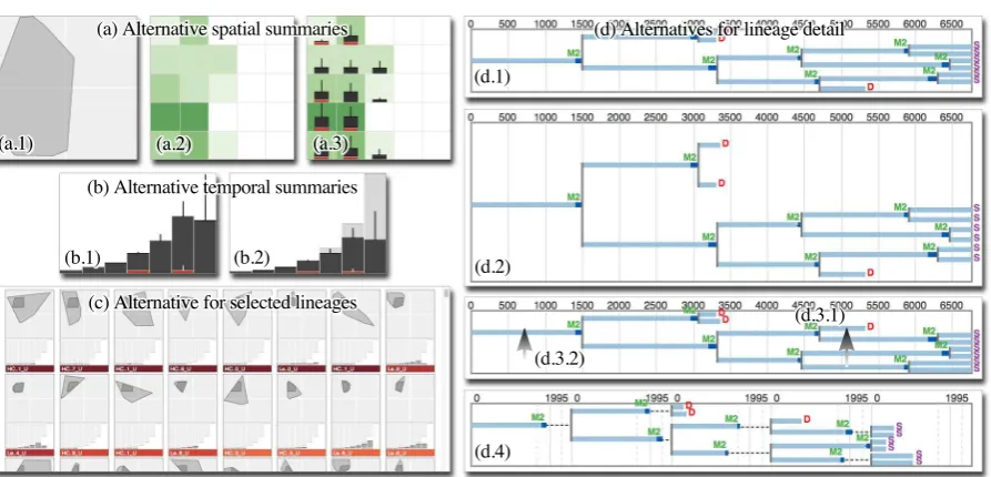
Figure 3:(a) Design alternatives for spatial summaries of grouped lineages. (a.1) The smallest convex polygon containing all key events gives no indication of different levels of activity. (a.2) Division into rectangular sub-regions with the average number of events shown as a heatmap. (a.3) For more precise analysis, the average number of events is redundantly encoded with the height of a bar in each region and standard deviation is shown with vertical error bars. The average number of cell deaths, an event type of great interest, is shown with the height of red bars. (b) Alternatives for temporal summaries of grouped lineages. (b.1) A bar chart where for every generation, the average number of key events and the standard deviation is shown. Cell deaths are in red. (b.2) To allow comparison of per-generation behaviour to an ideal scenario, the number of cell divisions for a lineage where every cell divides into two daughter cells, is shown in the background. (c) An alternative for visualising selected lineages as a scrolling list (compare to Figure4(d)). The area of intersection of their “footprints” with a user-specified lineage is computed and they are sorted in descending order of this area (dark grey). (d) Alternatives for visualising cell lineage detail. (d.1) Lineage laid out by elapsed time. (d.2) To emphasise the presence or absence of symmetry, a lineage can be laid out as it would be for a complete binary tree, but screen space is used very inefficiently. A more suitable approach is (d.3.1) to position the subtree with the smallest total inter mitotic time over all its descendants nearer the top at every branching point, and (d.3.2) centre parent nodes between direct child nodes and not between all descendants. (d.4) To highlight synchrony, the layout can be interactively changed to align nodes per generation. Average inter mitotic time±standard deviation is shown as vertical lines behind every generation. When multiple lineages are displayed, they share a temporal timescale on the x-axis.

4.2. Selections

Grouping and faceted navigation lets users identify and se-lect subsets of lineages corresponding to particular scenar-ios, for example, a particular drug and concentration. Users can also interact with collections of lineages independently of the number of individual lineages (assuming adequate hardware support). Moving the cursor over an icon brings it in focus by highlighting (see Figure4(b)). All other groups that contain lineages in the focus group are also highlighted so users can inspect the distribution of lineages in terms of metadata. All highlighted icons are selected when users click or tap their input device. Selections are refined using stan-dard interaction techniques to add or remove groups of lin-eages. A coloured gauge below each icon shows the number of lineages selected as a ratio of group size. Unselected lin-eages can be filtered out (Figure4(c)).

Initially, all selected lineages were shown in full detail (see Section4.3below), but domain experts found this over-whelming. They indicated that they prefer concise descrip-tions of the individual selected lineages to then pick lineages to view in detail. To achieve this, we reuse the spatiotem-poral icons described in Section4.1. A user selection can contain large numbers of lineages and we considered alter-natives to display their icons.

accord-ing to how similar their spatial summaries are to a uniformly dense heatmap, or how similar their generation sizes are to those of a perfect lineage (a complete binary tree). Users navigate between pages of icons in terms of an understood sorting metric to select individual lineages to view in detail.

4.3. Structural detail

When users select individual lineages from the paginated icons, they are shown in detail (see Figure4(e)). For this, do-main experts had an outspoken preference for directed node-link diagrams, a de-facto standard due their use for depicting cell lineages in print publications (for example, [KHCe07]). We use a left-to-right orientation to conform to our col-laborators’ preferred convention when including lineage di-agrams in reports and articles, and to be consistent with our generation-based temporal summaries (see Section4.1). We started by visualising a cell lineage by elapsed time, using the conventions described in Section2.6(see Figure3(d.1)). Every cell is represented by a horizontal track of which the length depicts its inter mitotic time. A cell birth event re-sults in two daughter cell tracks branching from the mother cell’s track. We use vertical connectors between mother and daughter cells to align their temporal intervals. Cellu-lar events are indicated by colour-coded text labels. When multiple lineages are selected, they are vertically juxtaposed on the same timescale to facilitate comparison.

A cell can be in one of several phases, for example, our current data distinguishes between theI-phase (interphase), when a cell grows and DNA is duplicated, andM-phase (mi-tosis), when it divides. We colour-code these phases on every track in light and dark blue, respectively (see Figure3(d)). As higher fidelity data becomes available, this approach can be extended to show more detailed cell-phase data, for ex-ample, interphase can be further subdivided intoG1-,S-, and

G2-phases. Users can also select any derived attribute to map

onto the cell tracks. Our software determines the type of data (nominal, ordinal, or numerical) and chooses an appropriate colour-map accordingly.

Symmetry.To let users analyse symmetry, we considered different approaches. We first positioned nodes as they would be for a complete binary tree of the same height (cor-responding to a scenario where every cell division leads to two daughter cells). This highlights the presence or absence of symmetry, but at the cost of significant display space (see Figure 3(d.2)). Because domain experts routinely wish to analyse several lineages simultaneously, this is not desirable. As an alternative, we make two simple adaptations to Reingold and Tilford’s “tidy” algorithm, a standard tree lay-out for directed node-link diagrams [RT81]. First, we sort the subtrees at each branching point so that the subtree with the shortest total inter mitotic length (the sum for all its de-scendants) is positioned nearer the top (see Figure3(d.3.1)). This already improves the ability to identify the presence

or absence of symmetry in a consistent way. Second, the tidy algorithm attempts to ensure that the layout and its mir-ror image are similar by positioning nodes vertically at the geometric centre of all of their descendants (when laid out left-to-right). To prevent asymmetric trees from being drawn symmetrically, we position every node vertically at the cen-tre of its direct child nodes (Figure3(d.3.2)). Our collabora-tors were enthusiastic about these subtle changes. We argue that they offer an effective compromise for addressing sym-metry without the wasted space of our initial approach.

Synchrony.To address our synchrony requirement, we de-veloped a technique where, with a lineage from left-to-right, tracks corresponding to every generation are aligned at the left and visualised on vertical bands of equal width (see Fig-ure3(d.4)). For a single lineage, the width of the bands is de-termined by the longest track in the lineage. When multiple lineages are selected, the width is determined by the longest track in all the lineages and used in all visualisations. Dashed lines connect nodes where the track length is less than this maximum. This approach enables users to compare the de-gree of synchrony within individual generations and, when several lineages are selected, across lineages.

To further support comparison, the average (mean) inter mitotic time and standard deviation are computed for each lineage and drawn as vertical lines behind every generation (average: solid; average±standard deviation: dashed). This

provides further context for analysis which, by comparing horizontal distances to references, is less arduous and quanti-tatively more precise, while providing information on the de-gree of variation (an important capability noted previously).

Spatial field.Biologists occasionally want to see if there are similar spatial patterns or interaction between cells that share the same field of observation. To allow for this, we include a view where the branching structures of selected lineages are shown in a representation of the spatial field (see Fig-ure4(f)). It is linked to all other views so users can investi-gate spatial movement in relation to other data properties.

4.4. Implementation

We implemented our approach in a system called Cell-o-pane [Cel], using Javascript and the D3.js visualisation li-brary [BOH11]. It runs in any modern web browser and reads cell lineages in JSON data format, where every cell is described by the properties outlined by Khan [Kha08].

5. Case study - cytotoxicity of an anticancer agent

A. J. Pretorius, I. A. Khan, & R. J. Errington / Cell lineage visualisation 7

action. The objectives of this study were to understand the dynamics of cell death and to identify and characterise cell survival strategies.

Data were obtained as follows. The parental cell line U-2 OS cells (osteocarcoma, a type of bone cancer) were derived from a 15 year old Caucasian female U-2 OS (ATCC HTB-96). Cells were seeded and plated onto a 6-well plate, left for 24h at 37◦_{C and 5% CO2using standard tissue culture}

techniques. Cells were then exposed to a bolus treatment of topotecan (a discrete exposure for 1 hour at a concentration of 10µM) or left untreated (control). Plates were placed onto a wide-field time-lapse instrument designed to capture trans-mission phase image sequences. Images were captured every 15min for 144h at 512×512 pixels. Cell lineages were de-rived by image processing, including cell tracking and semi-automated event detection [KHCe07]. The description below was derived from a diary kept during analysis.

5.1. Overview

Two analysts considered 85 control and 85 topotecan-treated lineages (10µM). Figure4(g) summarises their behaviour

us-ing our prototype’s spatiotemporal icons, obtained by select-ing and groupselect-ing on the “drug” metadata field.

The spatial summaries reveal much more activity under control conditions (a high average of cellular events per re-gion maps to a darker colour and taller bar compared to a low average; see Section4.1). There is also a much larger degree of variation of number of events for the control (tall error bars). These observations are confirmed by the tem-poral summaries at the bottom of each icon. Significantly, the ratio of cell death events (in red) compared to regular events is higher for the treatment condition. These observa-tions enabled the analysts to confirm that topotecan reduces the number of regular cellular events (cell division) and that under treatment, cell death is a much more prominent event.

5.2. Control condition

Next, using our prototype’s selection mechanism, the an-alysts picked 12 lineages for closer analysis. Figure4(h) and (i) show the lineages’ structural detail using the visu-alisation described in Section4.3(event types are colour-coded). Aligning tracks by generation, it is clear that for the control, early generations are synchronised in terms of cell cycle time (branch lengths), while at later generations they become asynchronous as inter mitotic time varies stochasti-cally. This behavioural heterogeneity accounts for the high degree of variation in the summary views noted above.

Another important observation regarding the control re-lates to unusual events. This includes polyploid events, where a cell commits to mitosis but does not separate into two daughter cells (see Figure4(h.1)) and refusion, where a cell refuses to divide (Figure4(h.2)). It was recently shown

that osteocarcoma cells have a tendency to carry an innate burden of polyploid cells [DdL11]. Based on this, polyploid mitosis and refusion were expected in the control data. Our visualisation provided the capacity for detecting the lineage location of a polyploid event and, importantly, the ability to determine the lead-up and consequences of such events.

5.3. Treatment condition

Treatment with a high dose of topotecan (10µM) not only contrasts with the control condition by removing polyploid events, but also leads to cytotoxicity. The location and pat-terns of cell death, including its relation to symmetry and synchrony, provided a means for determining three patterns of cytotoxicity. First is primary cytotoxicity, where the pri-mary event of the progenitor cell is cell death in generation 0 (see Figure4(i.1)). From this, the analysts inferred that the cells have a high cytotoxicity index and that they were prob-ably in S-phase upon treatment (when DNA duplicates). Pri-mary cytotoxicity is an ideal situation where tumour cells are terminated effectively without any potential for cell survival. A second pattern, symmetrical cytotoxicity, involves both siblings dying some time after cell division. Figure4(i.2) shows how a lineage initially expands, but all progeny die in generation 2, after considerable cell cycle delay in gen-eration 1. This is interesting because there is a capacity and opportunity for cell survival. An understanding of why cell death occurs symmetrically across all progeny, but only at generation 2 is an open question and requires more research. Third, with asymmetrical cytotoxicity, one sibling dies while the other survives (see Figure4(i.3)). The analysts identified the emergence of drug-resistant progeny, where despite the death of one sibling, a resistant track survives. By generation 4, the surviving progeny become apparent and the visualisations show their contiguous events. Accrual of drug resistance in tumour cells as a survival strategy under cancer treatment is a recurring theme in drug discovery and cancer research. This case study clearly shows the temporal escape patterns of subpopulations of cells that emerge from cytotoxic burden and highlights that their origin and growth patterns are unknown, requiring more research.

6. Discussion and conclusion

A. J. Pretorius, I. A. Khan, & R. J. Errington / Cell lineage visualisation 9

Section2.1). Although they had found isolated cases of cyto-toxicity, it was impossible to maintain an overview and keep track of the behaviour or multiple cells and their progeny. In particular, symmetrical and synchronous patterns were not revealed, nor could they be compared across lineages. These shortcomings, and those noted in Section2, are exacerbated as the number of cells in experiments increases.

In contrast, our approach enabled comprehensive analy-sis. First, analysts could take account of the multimodal-ity of cell lineages (see Section3.1). They could consider metadata, spatiatemporal data, and cellular event locations (polyploidy, refusion, and cell death) to analyse cytotoxic-ity in the developmental context of whole lineages. Second, they could observe the presence or absence of symmetry and synchrony (Sections3.2and3.3), and analyse the biological implications of these phenomena across multiple lineages. For example, classes of behaviour resulting from drug treat-ment were identified and characterised. This illustrates how our approach addresses the requirements identified in Sec-tion3. In addition, the analysts found it valuable for present-ing results, notpresent-ing that it is hard to match the effectiveness of graphically illustrating findings such as the asymmetric es-cape strategy from cytotoxicity in Figure4(i.3). At the time of writing, we are preparing a manuscript that focuses on the implications of our work on biomedicine that makes promi-nent use of visualisations generated by our prototype.

There are other scenarios where lineage visualisation can play a role. Quality control (QC) is a critical but challeng-ing part of the high-throughput paradigm [BFHea12]. In-spection of behavioural summaries of cell lineages that show variation and error, and the ability to compare multiple lin-eages offer a way to identify problems and ensure reliabil-ity. Visualisation can also reduce the significant effort re-quired to test and validate mathematical models of cellu-lar behaviour [GLHR09]. Further, despite the exponential growth of biocuration infrastructure and databases, reuse of data beyond the originator remains rare due to idiosyncratic methodologies. Our prototype has enabled analysts to un-derstand similarities and differences in experiment design by grouping on metadata and considering results. There is currently no other support for this kind of analysis.

We now reflect on more general lessons learned. First, the requirement of showing variation in our spatial, tempo-ral, and structural visualisations highlights the importance of visualising variation and uncertainty (see Figure3(a), (b), (d.4)). This is an often overlooked challenge [SLSR10]. Sec-ond, our users requested that the generation sizes of idealised lineages also be shown as contextual information in our tem-poral summaries (Figure3(b.2)). Like others, we found sub-tle changes to show “prior knowledge” to be advantageous for ensuring correct interpretations [Che05]. Third, our users preferred spatio-temporal icons to be presented in a pagi-nated fashion and not as scrolling lists, which conforms to research results [SW09]. A recurring theme, based on expert

feedback, was to sort icons according to an understood cri-terion so users understand what lineages near the start, mid-dle, and end have in common. Fourth, although a previous study found users to prefer a top-to-bottom orientation for node-link diagrams [BKHe11], our users had a definite pref-erence for a left-to-right layout. This stresses the importance of context-of-use in designing visualisations.

We have successfully analysed up to two thousand lin-eages with our method. This is an important improvement on previous methods that support analysis of either high-level aggregates or a handful of individual lineages. In particular, our aggregate visualisations are scale-free to enable users to drill down from high- to detail-level in a flexible fashion. Al-though our focus has been on front-end visualisation design, substantial scalability improvements can be realised by im-plementing a back-end that serves aggregate data and subsets of lineage data based on user interaction.

There are also other opportunities for improving our ap-proach. Analysts have found the sorted presentation of in-termediate selections useful (see Section4.2). However, a solution that allows more flexible sorting based on multi-ple criteria could make better use of multimulti-ple measures that are routinely derived. Linking visual analysis to the underly-ing image data would also be an advantage. As cell trackunderly-ing algorithms improve, we expect that multivariate time-series that describe individual cell cycles will become available (as opposed to the monolithic tracks we currently have). Map-ping such data onto cell lineages will yield high fidelity de-scriptions of the development of cells. Based on our experi-ence, we argue that visualisation can play a significant role in unlocking the value of such data. However, more work is re-quired to develop methods that integrate rich spatial, tempo-ral, multivariate, and hierarchical data. The work presented here is an important first step in addressing this challenge.

Acknowledgements

We thank Mark Bray and Anne Carpenter (Broad Insti-tute), Tatiana von Landesberger (Darmstadt), Roy Ruddle (Leeds), and Nick White (Cardiff). Pretorius was supported by a Leverhulme Early Career Fellowship (ECF2012-071), Khan and Errington by a BBSRC Sparking Impact Award (BB/E012574/1).

References

[AA13] ANDRIENKON., ANDRIENKOG.: Visual analytics of movement: an overview of methods, tools and procedures. Infor-mation Visualization 12, 1 (2013), 3–24.3

[BFHea12] BRAY M. A., FRASER A. N., HASAKA T. P.,

ET AL.: Workflow and metrics for image quality control in

large-scale high-content screens.J. Biomol. Screen. 17, 2 (2012), 266– 274.9

[BOH11] BOSTOCKM., OGIEVETSKYV., HEERJ.: D3: data-driven documents. IEEE Trans. Vis. Comput. Graph. 17, 12 (2011), 2301–2309.6

[Bre] BREWERC. A.: ColorBrewer. www.colorbrewer. org. Accessed October 2014.4

[BvLHe11] BREMMS.,VONLANDESBERGERT., HESSM.,ET AL.: Interactive visual comparison of multiple trees. InIEEE Conf. Visual Analytics Science and Technology(2011), pp. 31– 40.3

[Car07] CARPENTERA. E.: Image-based chemical screening. Nat. Chem. Biol. 3, 8 (2007), 461–465.1

[CECe08] CHEUNGS. Y., EVANSN. D., CHAPPELLM. J.,ET AL.: Exploration of the intercellular heterogeneity of topotecan uptake into human breast cancer cells through compartmental modelling.Math. Biosci. 213, 2 (2008), 119–134.3

[Cel] Cell-o-pane. www.comp.leeds.ac.uk/scsajp/ applications/cell-o-pane/. Last accessed 6 March 2015.6

[Che05] CHENC.: Top 10 unsolved information visualization problems.IEEE Comput. Graph. Appl. 25, 4 (2005), 12–16.9

[CJLe06] CARPENTERA. E., JONEST. R., LAMPRECHTM. R.,

ET AL.: CellProfiler: image analysis software for identifying and

quantifying cell phenotypes.Genome Biol. 7(2006), R100.1

[DdL11] DAVOLI T., DE LANGE T.: The causes and conse-quences of polyploidy in normal development and cancer.Annu. Rev. Cell Dev. Biol. 27(2011), 585–610.8

[ECKe13] ERRINGTONR. J., CHAPPELLS. C., KHANI. A.,ET AL.: Time-lapse microscopy approaches to track cell cycle and lineage progression at the single-cell level.Curr. Protoc. Cytom. 12, 4 (2013).1

[Fod02] FODORI. K.: A survey of dimension reduction tech-niques. Tech. Rep. UCRL-ID-148494, Lawrence Livermore Na-tional Laboratory, 2002.2

[GBBS09] GORDONJ. L., BUGULISKISJ. S., BUSKEP. J., SIB

-LEYL. D.: Actin-like protein 1 (ALP1) is a component of dy-namic, high molecular weight complexes in toxoplasma gondii. Cytoskeleton 67, 1 (2009), 23–31.2

[GK10] GRAHAMM., KENNEDYJ.: A survey of multiple tree visualisation.Information Visualization 9, 4 (2010), 235–252.3

[GLHR09] GLAUCHE I., LORENZ R., HASENCLEVER D.,

ROEDERI.: A novel view on stem cell development: analysing

the shape of cellular genealogies.Cell Prolif. 42, 2 (2009), 248– 263.1,2,3,9

[Häg70] HÄGERSTRANDT.: What about people in regional sci-ence?Pap. Reg. Sci. 24, 1 (1970), 7–24.2

[HLLK09] HSU Y. Y., LIUY. N., LU W. W., KUNG S. H.: Visualizing and quantifying the differential cleavages of the eu-karyotic translation initiation factors eIF4GI and eIF4GII in the enterovirus-infected cell. Biotechnol. Bioeng. 104, 6 (2009), 1142–1152.2

[HMM00] HERMAN I., MELANÇON G., MARSHALL M. S.: Graph visualization and navigation in information visualization: a survey.IEEE Trans. Vis. Comput. Graph. 6, 1 (2000), 24–43.2

[HWKT09] HAMILTONN. A., WANGJ. T. H., KERRM. C.,

TEASDALER. D.: Statistical and visual differentiation of

sub-cellular imaging.BMC Bioinformatics 10(2009), 94.2

[Jen13] JENSENE. C.: Overview of live-cell imaging: require-ments and methods used.Anat. Rec. 296, 1 (2013), 1–8.1

[JKWe08] JONEST. R., KANGI. H., WHEELERD. B.,ET AL.: CellProfiler Analyst: data exploration and analysis software for

complex image-based screens. BMC Bioinformatics 9(2008), 482.2

[Kha08] KHANI. A.: A novel bioinformatics approach for en-coding and interrogating the progression and modulation of the mammalian cell cycle. PhD thesis, Dept. Pathology, Cardiff Uni-versity, 2008.1,6

[KHCe07] KHANI. A., HUSEMANNP., CAMPBELLL.,ET AL.: ProgeniDB: a novel cell lineage database for generation associ-ated phenotypic behavior in cell-based assays. Cell Cycle 6, 7 (2007), 868–874.2,3,6,8

[KLCe11] KHANI. A., LUPIM., CAMPBELLL.,ET AL.: In-teroperability of time series cytometric data: a cross platform ap-proach for modeling tumor heterogeneity. Cytometry A 79, 3 (2011), 214–226.3

[LKBe14] LENZO., KEULF., BREMMS.,ET AL.: Visual anal-ysis of patterns in multiple amino acid mutation graphs. InIEEE Conf. Visual Analytics Science and Technology(2014), pp. 93– 102.3

[PM07] PRASADM., MONTELLD. J.: Cellular and molecular mechanisms of border cell migration analyzed using time-lapse live-cell imaging.Dev. Cell. 2, 6 (2007), 997–1005.1

[Pom06] POMMIERY.: Topoisomerase I inhibitors: camptothe-cins and beyond.Nat. Rev. Cancer 6, 10 (2006), 789–802.6

[PvW09] PRETORIUSA. J.,VANWIJKJ. J.: What does the user want to see? What do the data want to be? Information Visual-ization 8, 3 (2009), 153–166.3

[RT81] REINGOLDE. M., TILFORDJ.: Tidier drawings of trees. IEEE Trans. Softw. Eng. SE-7, 2 (1981), 223–228.6

[Sch11] SCHULZ H.-J.: Treevis.net: a tree visualization refer-ence.IEEE Comput. Graph. Appl. 31, 6 (2011), 11–15.3

[SHTe12] SCHERFN., HERBERGM., THIERBACHK.,ET AL.: Imaging, quantification and visualization of spatio-temporal pat-terning in mESC colonies under different culture conditions. Bioinformatics 28, 18 (2012), i556–i561.2,3

[SLSR10] SKEELSM., LEEB., SMITHG., ROBERTSONG.: Re-vealing uncertainty for information visualization. InWorking Conf. on Advanced Visual Interfaces(2010), pp. 376–379.9

[SMCe06] SIGALA., MILOR., COHENA.,ET AL.: Dynamic proteomics in individual human cells uncovers widespread cell-cycle dependence of nuclear proteins.Nat. Methods 3, 7 (2006), 525–531.2

[SMKM10] SANTIAGO-MOZOS R., KHAN I. A., MADDEN

M. G.: Revealing the origin and nature of drug resistance of dynamic tumour systems.Int. J. Knowledge Discovery in Bioin-formatics 1, 4 (2010), 26–53.3

[SW09] SANCHEZC. A., WILEYJ.: To scroll or not to scroll: scrolling, working memory capacity, and comprehending com-plex texts.Hum. Factors 51, 5 (2009), 730–738.9

[Tuf90] TUFTE E.: Envisioning Information. Graphics Press, 1990.4

[Tun09] TUNKELANGD.:Faceted search. Morgan and Claypool Publishers, 2009.4

[War01] WAREC.: Designing with a 2 1/2-D attitude. Informa-tion Design J. 10, 3 (2001), 255–262.2

[WHNe09] WALTERT., HELDM., NEUMANNB.,ET AL.: Au-tomatic identification and clustering of chromosome phenotypes in a genome wide RNAi screen by time-lapse imaging.J. Struct. Biol. 170, 1 (2009), 1–9.2