Accounting for Uncertainty in Confounder and Effect Modifier Selection When Estimating Average Causal Effects in Generalized Linear Models

(1)

Accounting for Uncertainty in Confounder

and Effect Modifier Selection When

Estimating Average Causal Effects

in Generalized Linear Models

The Harvard community has made this

article openly available.

Please share

how

this access benefits you. Your story matters

Citation

Wang, Chi, Francesca Dominici, Giovanni Parmigiani, and Corwin

Matthew Zigler. 2015. “Accounting for Uncertainty in Confounder and

Effect Modifier Selection When Estimating Average Causal Effects

in Generalized Linear Models.” Biometrics 71 (3): 654–65. https://

doi.org/10.1111/biom.12315.

Citable link

http://nrs.harvard.edu/urn-3:HUL.InstRepos:37933091

Terms of Use

This article was downloaded from Harvard University’s DASH

(2)

Accounting for Uncertainty in Confounder and Effect Modifier

Selection when Estimating Average Causal Effects in

Generalized Linear Models

Chi Wang1,2,*, Francesca Dominici3, Giovanni Parmigiani3,4, and Corwin Matthew Zigler3

1_{Department of Biostatistics, University of Kentucky, Lexington, KY, USA} 2_{Markey Cancer Center, University of Kentucky, Lexington, KY, USA}

3_{Department of Biostatistics, Harvard School of Public Health, Boston, MA 02115, USA}

4_{Department of Biostatistics and Computational Biology, Dana-Farber Cancer Institute, Boston,}

MA 02115, USA

Summary

Confounder selection and adjustment are essential elements of assessing the causal effect of an exposure or treatment in observational studies. Building upon work by Wang et al. (2012) and Lefebvre et al. (2014), we propose and evaluate a Bayesian method to estimate average causal effects in studies with a large number of potential confounders, relatively few observations, likely interactions between confounders and the exposure of interest, and uncertainty on which

confounders and interaction terms should be included. Our method is applicable across all exposures and outcomes that can be handled through generalized linear models. In this general setting, estimation of the average causal effect is different from estimation of the exposure coefficient in the outcome model due to non-collapsibility. We implement a Bayesian bootstrap procedure to integrate over the distribution of potential confounders and to estimate the causal effect. Our method permits estimation of both the overall population causal effect and effects in specified subpopulations, providing clear characterization of heterogeneous exposure effects that may vary considerably across different covariate profiles. Simulation studies demonstrate that the proposed method performs well in small sample size situations with 100 to 150 observations and 50 covariates. The method is applied to data on 15060 US Medicare beneficiaries diagnosed with a malignant brain tumor between 2000 and 2009 to evaluate whether surgery reduces hospital readmissions within thirty days of diagnosis.

Keywords

Average causal effect; Confounder selection; Treatment effect heterogeneity; Bayesian adjustment for confounding

*_{[email protected].}

6. Supplementary Materials

Web Appendices and Tables referenced in Sections 2, 3 and 4 and the code implementing BAC are available with this paper at the

HHS Public Access

Author manuscript

Biometrics. Author manuscript; available in PMC 2015 September 18.

Published in final edited form as:

Biometrics. 2015 September ; 71(3): 654–665. doi:10.1111/biom.12315.

Author Manuscript

(3)

1. Introduction

Assessing the causal effect of an exposure, or treatment, on an outcome is a common goal in many observational studies. Since the exposure is not randomly assigned, individuals with different levels of exposure may differ systematically in baseline variables related to both the exposure and the outcome, or confounders. Estimation of the average causal effect (ACE) of the exposure on an outcome requires adjustment for confounders, but many observational studies contain a large number of observed baseline variables, and there is often uncertainty about which of these potential confounders are required for adjustment. The bias and variance of the ACE estimate can depend strongly on which variables are included for adjustment, and it is challenging to select and adjust for the right set of confounders from a large set of candidates.

An important related problem to prioritizing potential confounders is how to estimate causal effects that vary as a function of baseline characteristics. This is sometimes referred to as treatment effect heterogeneity (TEH). Kurth et al. (2006) and Lunt et al. (2009) showed that when the causal effect of exposure on an outcome is heterogeneous, different estimation methods may yield extremely different exposure effect estimates, illustrating the need for great care about the choice of methods and the interpretation of the results. These difficulties are amplified when the set of baseline variables is large and there is uncertainty regarding which factors may interact with the exposure.

We propose new methods that can a) prioritize which observed covariates are genuine confounders of causal effects, and b) transparently characterize effect modification for specific study populations. As an example that motivates this study, we use U.S. Medicare beneficiary data to evaluate the causal effect of surgery on hospital readmission rates among elderly individuals diagnosed with malignant brain tumors. Many factors, such as

demographic characteristics and comorbid conditions, may confound the surgery effect, and it is also suspected that patients with different characteristics may respond to surgery differently.

Our approach builds upon work by Wang et al. (2012), who proposed a method called Bayesian Adjustment for Confounding (BAC) to account for the uncertainty in confounder selection when estimating the relationship between a continuous exposure and a continuous outcome with a linear regression model. The BAC method jointly considered two models: (1) an exposure model regarding the exposure as a function of potential confounders; and (2) an outcome model regarding the outcome as a function of the exposure and potential confounders. Rather than base inference on a single model specification, BAC applies Bayesian model averaging (BMA, Raftery et al. (1997)) to average inference across many model according to posterior support from the data. Whereas standard BMA assigns posterior weight primarily to outcome predictors, BAC is based on a joint model prior to consider potential confounders’ association with both the exposure and the outcome and assign large posterior weights to models including all the true confounders. BAC was extended to binary exposures by Lefebvre et al. (2014), but has not been used for general types of outcomes or for the purposes of identifying and estimating TEH.

Author Manuscript

(4)

In this paper, we extend and generalize the BAC method (Wang et al., 2012; Lefebvre et al., 2014) to any exposure and outcome that can be handled by generalized linear models (GLMs) and consider interactions that constitute TEH. In contrast to the special case of linear regression, where the exposure coefficient in the outcome model corresponds to the ACE in certain circumstances (Schafer and Kang, 2008), estimation of ACEs in GLMs differs from estimation of a single model coefficient because of non-collapsibility, that is the fact that the meaning and magnitude of exposure coefficient changes by adding or removing a variable unrelated to the exposure (Greenland et al., 1999; Vansteelandt, 2012). We propose a procedure to estimate ACEs by comparing the predicted outcome values between different exposure levels. The formula involves an integral over the distribution of

confounders, which is estimated non-parametrically using a Bayesian bootstrap procedure. By including the possibility of interactions with the exposure, our method clearly indicates which confounders interact with the exposure and how, which characterizes TEH in scientifically-interpretable subgroups. The proposed approach can estimate the ACE for the whole population or for a given subpopulation of interest, e.g. patients from a certain age group.

Our generalized BAC method (henceforth BAC for brevity) shares important points of contact with methods based on propensity scores (Rosenbaum and Rubin, 1983; Imai and Van Dyk, 2004; Lunceford and Davidian, 2004; McCandless et al., 2009) in that it makes explicit use of a model predicting exposure, conditional on covariates (i.e., a propensity score model), and the target for inference is the ACE, possibly in population subgroups. Whereas typical propensity score methods estimate the ACE by comparing outcomes from exposed and unexposed individuals with similar estimated propensity scores, BAC estimates the ACE with a parametric outcome regression model that does not explicitly contain the propensity score, but rather uses the propensity score model to guide the inclusion of confounders in the outcome model.

Confounder selection is a critical issue for propensity score methods as well. When sample size permits, it is recommended to include into the propensity score model genuine confounders associated with exposure and outcome, as well as variables unrelated to the exposure but predictive of the outcome (Brookhart et al., 2006; Schafer and Kang, 2008). In smaller samples, however, inclusion of extraneous baseline variables comes at the cost of efficiency and the risk of separating the covariate distributions in exposure groups to the extent that they no longer overlap (Schafer and Kang, 2008). Data-driven methods to select variables to include in propensity score models are emerging. When exposure, outcome, and potential confounders are all binary, Schneeweiss et al. (2009) proposed an algorithm to rank potential confounders for inclusion in the propensity score model. When both exposure and outcome are binary, Zigler and Dominici (2014) proposed Bayesian methods for variable selection and model-averaged causal effect estimation with propensity scores that share important similarities with BAC. To our knowledge, there has not been a unified method that can handle uncertainty in confounder selection across different data types, and methods that account for uncertainty in the selection of population subgroups exhibiting TEH are nonexistent. The BAC method presented in this paper is intended to address these important practical barriers to causal inference in high dimensional settings where

propensity score methods are difficult to implement and interpret.

Author Manuscript

(5)

2. Methodology

2.1 The Causal Model

Let X be the exposure, Y be the outcome, and V be a set of M potential confounders V = {V1,

…, VM }. Both the exposure and the outcome variables can be binary, continuous, count or

other data type that can be handled by GLMs. Our goal is to estimate the ACE of X on Y, possibly within population subgroups, with adjustment for confounding. A priori, there may be uncertainty about which potential confounders should be adjusted for in the estimation as well as which baseline covariates might interact with the exposure.

Let Δ(x1, x2) represent the ACE of a change in X from x1 to x2. Formally, Δ(x1, x2) is defined

as a comparison between potential outcomes under competing exposure levels (Rubin, 1974). We forego potential-outcomes notation, and simply state the assumption of strongly ignorable treatment assignment (sometimes termed the “no unmeasured confounding assumption”), stating that potential outcomes are unrelated to levels of X, conditional on V. We further assume each unit has a positive probability of receiving any level of the exposure. This permits representation of Δ(x1, x2) as:

(1)

which can be estimated with observed data. The ACE is tied to the study population through the marginal distribution of V which could refer to the whole population or a specific subpopulation. We assume throughout that the confounders required for ignorability are an unknown subset of those available in V.

2.2 Bayesian Adjustment for Confounding (BAC)

We build our approach for estimating ACE via two collections of GLMs: one for exposure and one for outcome. Specifically, we consider the following equations:

(2)

where f(.) and g(.) are link functions and i indexes the sampling unit. In each equation, potential confounders are either included or excluded, depending on unknown vectors of

indicators αX_∈_{{0, 1}}M_and_αY_∈_{{0, 1}}2M_{. Here} _{whenever V}

m is included in the

exposure model. Similarly, whenever Vm is included and whenever the

interaction between Vm and X is included in the outcome model. In general, the number of

possible interactions (including higher order interactions) that could be specified in (2) is so large as to necessitate the specification of a reduced number of potential interactions. For illustration, we restrict attention to the two-way interactions between each V and X, but other interactions could be included in (2). For brevity, we refer to different choices of the parameters αs as “models”. For regression coefficients, β and δ, we use a notation that explicitly keeps track of the fact that those coefficients differ in meaning with the αs. Let

βαY be a vector of model parameters appearing in a certain outcome model αY_{. Our}

Author Manuscript

(6)

specification is an extension of the linear case considered in Wang et al. (2012) to GLMs that include interactions between exposure and confounders.

We calculate the ACE by BMA (Raftery et al., 1997) across all possible outcome models with the functional form expressed in equation (2):

(3)

where D = (Y, X, V) are the observed data and ΔαY (x1, x2) = EV {E(Y |X = x1, V, αY) – E(Y |

X = x2, V, αY)}. For a model αY that includes all the true confounders, Δα

Y

(x1, x2) is the

same as Δ(x1, x2). In contrast, Δα

Y

(x1, x2) may be different from Δ(x1, x2) if αY does not

include all the true confounders. Therefore, the second equation in (3) only holds

approximately, requiring that the posterior p(αY_{|D) concentrates on models that include all}

the true confounders, which motivates the joint modeling of exposure and outcome in equation (2). As we will describe in more detail in Section 2.3, a joint prior for αX_and_αY

favors inclusion of covariates correlated with both X and Y in the outcome model, which concentrates posterior mass on models including true confounders.

For a given outcome model αY_{, let h(X, V ;}_βαY

) be the linear function of X and V on the right hand side of the outcome model in equation (2). We have

(4)

When the outcome model is a linear regression without interactions between X and V,

ΔαY(x₁, x₂) is equal to . In general, such a clear connection between the model coefficient for exposure and ΔαY (x1, x2) is not available. The expression of Δα

Y

(x1, x2) in

equation (4) includes an integral over the distribution of V, which needs to be specified. This is different from regular GLM inference which is conditional on V, so the distribution does not need to be considered explicitly. To estimate the distribution of V, we use the Bayesian bootstrap (Rubin, 1981; Newton and Raftery, 1994). Suppose V takes K distinct values V1,

…, VK and let θ = (θ1, …, θK)T be the probabilities with which V takes these values. Then

ΔαY (x1, x2) can be expressed as a function, ψ, with parameters βα

Y

and θ

(5)

Plugging (5) into (3), we obtain the posterior of ACE as

(6)

Author Manuscript

(7)

2.3 Prior and Posterior Distributions

We first consider the prior specification for αY. Our goal is to adjust for confounders without

a priori certainty about which among a large set of potential confounders are required. We

are concerned with studies where the sample size is small or moderate compared to the number of potential confounders (the ratio of sample size to the number of potential confounders is 2:1 to 10:1). To fully take into account the associations between potential confounders with both the exposure and the outcome, we consider the joint prior distribution on (αX_,_αY_{) proposed by Wang et al. (2012)}

(7)

where ω∈ [1, ∞] is a dependence parameter controlling both the prior odds of including Vm

into the outcome model when Vm is included in the exposure model and the prior odds of

excluding V_m from the exposure model when V_m is not included in the outcome model. When ω equals one, this prior reduces to the regular BMA prior where no connection between exposure and outcome models is assumed. When ω is large, this prior increases the chance for predictors strongly correlated with X to be included in the outcome model. These predictors are most likely to be true confounders if they are also correlated with Y.

Therefore, the prior leads to a posterior distribution of αY_{that prioritizes models including}

all true confounders. See Wang et al. (2012) for more discussion. In the following, we focus on the case with ω = ∞, which maximizes the dependence between inclusion in the

exposure model and the outcome model.

Moving to interactions between the exposure and potential confounders, we restrict the outcome model space to models that include the main effect terms whenever an interaction is included, that is,

(8)

In words, if Vm is included as a main effect, then we allow even odds a priori that Vm is

included in an interaction; whereas if Vm is not included as a main effect, then it will not be

considered to be an interaction. An alternative prior that allows interactions between confounders and the exposure in absence of main effects is provided in Web Appendix I.

We assume a priori independence between βαY and θ and show that their posteriors are also independent (see Web Appendix A for the proof). Therefore, these two parameters can be sampled separately in a Monte Carlo (MC) algorithm. Details of the prior and posterior distributions for βαY and θ are provided in Web Appendix A.

2.4 Implementation

We obtain posterior samples of the ACE by Markov chain Monte Carlo (MCMC) sampling from the posterior distributions of αY_,_βαY

and θ, and equation (6). Our algorithm is:

Author Manuscript

(8)

1. Generate a MCMC sample of αY from p(αY |D) by sampling (αX, αY) from their joint posterior p(αX_,_αY_{|D) based on the MC}3_{method of Madigan et al. (1995).}

2. For each individual model αY_{, sample}_βαY

and θ from their posteriors independently, then calculate ψ(x1, x2; βα

Y

, θ) to obtain a sample of ΔαY (x1, x2),

with size equal to the frequency of αY in the sample from step (1).

3. Stack samples of ΔαY (x1, x2) from individual outcome models to form an

approximate sample of Δ(x1, x2).

Details of the MCMC sampling procedure are provided in Web Appendix B.

2.5 Relation to Propensity Score Methods

The exposure model in (2) for a binary X is effectively a propensity score model. However, BAC does not make explicit use of the propensity score when adjusting for confounding, and does not share several purported benefits of standard propensity score methods. Benefits of propensity score methods are often described in the context of using observational data to approximate the “design” and “analysis” stages of a randomized study (Rubin, 2007). Noted virtues of “designing” the approximate randomized study include the ability to check for common covariate support and balanced covariate distributions in exposed and unexposed units. The separate “analysis” stage estimates causal contrasts without complete reliance on a parametric outcome model. However, these benefits of propensity score methods are contingent upon the ability to reliably estimate the propensity score and assess balance and common support, which can be challenging with high dimensional covariate information. Including many covariates in the propensity score model can sacrifice efficiency and, in extreme cases, simply preclude the ability to reliably estimate the propensity score. BAC is designed to specifically address high dimensional settings while acknowledging model uncertainty in the prioritization of confounders. BAC does not separate the “design” from the “analysis.” It uses outcome data along with exposure data to prioritize confounders and determine model weights, but does so in an automated data-driven way that does not compromise objectivity. The purpose is to provide a fair evaluation of the confounding effect for each potential confounder because by definition, a confounder is associated with both the exposure and the outcome so that its impact should be evaluated based on the strength of associations with not only the exposure but also the outcome. The potential for BAC to focus inference on a reduced set of factors that are empirically determined to be important confounders, while accounting for model uncertainty, may offer efficiency gains relative to methods that include a high number of potential confounders. A further

distinction is that BAC is designed to identify specific factors that drive TEH through inclusion as interaction terms, whereas propensity score methods are useful for estimating effects that vary across levels of the propensity score. Without post-hoc analysis, the propensity score does not directly identify exactly which factors constitute population subgroups experiencing TEH.

To the extent that the proposed method’s reliance on a parametric model eschews many common benefits of standard propensity score methods, it does so in an effort to address practical challenges to making causal inference in high dimensional settings (a) where the number of available covariates is large enough so as to compromise or even preclude the

Author Manuscript

(9)

ability to reliably deploy propensity score methods and (b) where interest lies in identifying specific observed factors that constitute a basis for TEH. We revisit differences between BAC and propensity score methods in the Discussion.

3. Simulation Studies

We conducted simulation studies to assess the performance of BAC and compare it to 1) the true outcome model; 2) the full outcome model including all the potential confounders and interactions; 3) the stratification by propensity score method; 4) the generalized boosted weighting method proposed and implemented with the R package twang (Ridgeway et al., 2014); 5) the high dimensional propensity score approach of Schneeweiss et al. (2009); and 6) an Ad hoc method that starts with the full model and performs backward selection based on the percentage change in the exposure coefficient with or without a potential confounder. For BAC, we considered a uniform prior for βαY (BACN, where “N” stands for

non-informative). And when the outcome is binary, we also considered a more informative prior described in Web Appendix A (BACI, where “I” stands for informative). For the

stratification by propensity score method, observations are stratified into five strata based on the quintiles of the estimated propensity score, and the ACE is estimated by a weighted sum of stratum-specific ACE estimates. We considered four variations of this method: a) a “full” model that estimates the propensity score using all potential confounders and then estimates the stratum-specific ACE as the difference of sample means of the outcome for each exposure (PSF, where “F” stands for full model); b) a “selected” model that estimates the

propensity score with backward stepwise selection and then estimate the stratum-specific ACE with the difference of sample means of the outcome for each exposure level (PSS,

where “S” stands for selected model); c) a method that augments the full model approach with regression adjustment by fitting an outcome regression model adjusting for all potential confounders within each propensity score stratum and estimates the stratum-specific ACEs with the average difference in predicted values comparing exposure levels (PSRF, where “R”

stands for regression adjustment within stratum); and d) a method that augments the selected model approach with regression adjustment by performing backward stepwise selection within each propensity score stratum and then estimates the stratum-specific ACE by the average difference in predicted values comparing exposure levels from the “selected” within-stratum regression (PSRS). For the twang method, a generalized boosted regression is

used to estimate the propensity scores. We considered three variations of inverse probability weighting with twang estimates to estimate the ACE: a) by the difference between weighted means of the observed outcomes for exposure groups (twangN, where “N” stands for

non-doubly robust); b) by a non-doubly robust estimator (Lunceford and Davidian (2004), equation (9)) incorporating an outcome regression model that includes all potential confounders (twangF, where “F” stands for full regression model); and c) by an estimator similar to the

one in b), but the outcome regression model only includes potential confounders that do not achieve balance (based on a Kolmogorov-Smirnov test in twang package) after inverse probability weighting (twangS, where “S” stands for selected model). For the Ad hoc

method, we considered 1% (Ad hoc1) or 5% (Ad hoc5) change in the exposure coefficient as

the criterion of confounder selection. Since the approach of Schneeweiss et al. (2009) only deals with the situation where exposure, outcome, and potential confounders are all binary

Author Manuscript

(10)

and the Ad hoc method is only valid when there is no TEH, they are only included when the simulation scenario is appropriate. Web Table 10 lists methods compared under each simulation scenario.

Our first scenario considers 50 potential confounders (V₁ to V₅₀) independently generated from N(0, 0.52) having varying strengths of association with exposure and outcome and no interaction terms. Binary exposure and binary outcome variables were generated from

Web Table 1 summarizes the values of the regression coefficients. In this scenario, V1

through V9 are true confounders with different strengths of associations with the exposure

and the outcome. This scenario also includes three other predictors of Y (V10 through V12)

that are not associated with X. We generated 500 independent simulation replicates for each sample size n = 100, 150, 300, or 500.

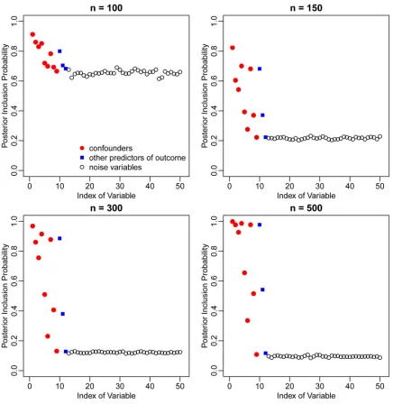
Figure 1 illustrates the marginal posterior inclusion probabilities (PIPs) assigned by BAC to each of the 50 potential confounders, averaged over simulation replicates. The PIP of the

mth potential confounder is defined as and is estimated by the

proportion of posterior samples of αY_{that includes the mth potential confounder. The PIPs}

of true confounders (V1—V9, red dots) are higher than those of other covariates not in the

outcome model (V13—V50, black circles). Higher PIPs are also assigned to other predictors

of the outcome (V10—V12, blue squares). The difference in PIPs between true predictors and

“noise variables” becomes larger as sample size increases. These results show that BAC identifies important variables in accordance with associations with both exposure and outcome. For example, V1, V2 and V3 have high PIPs due to their strong association with the

exposure. The PIP of V1 is even higher due to its strong association with the outcome.

Next, we compare the estimation of ACE from BAC, stratification by propensity score (PSF,

PSS, PSRF, and PSRS), the twang method (twangN, twangF, and twangS), the Ad hoc method,

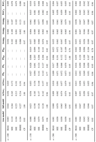
the true model, and the full model. For BAC, the MCMC chain ran for 2,500,000 iterations after 10,000 burn-in iterations. The thinning interval was set to 250 to reduce dependence among iterations. Simulation results are summarized in Table 1. The “true” ACE value was calculated based on a simulated data set with extremely large sample size (n = 10, 000, 000). The estimation of ACE based on BAC is virtually unbiased. The coverage probability (CP) for 95% credible interval is close to the desired value. The root mean square error (RMSE) from BACI is close to that from the true model, and smaller than those from all other

methods. Interestingly, the stratification method with subsequent regression adjustment within subclasses (PSRF and PSRS) has worse performance than the stratification method

without regression adjustment (PSF and PSS). This is because the stratification method with

regression adjustment requires larger sample size to achieve stable results due to the inclusion of many parameters in the within-stratum regression models.

Author Manuscript

(11)

For the smallest sample size considered (n = 100), BAC requires some stabilization via an informative prior distribution. While BAC_N does not provide stable results due to flatness of likelihood functions in some outcome models, the informative prior in BAC_I achieves the desired CP, with RMSE smaller than those from the true model and all the variations of the twang method. The prior in BAC_I has wide spread, and only serves to reduce prior support for unreasonably large coefficient values. So it seems that the instability in parameter estimation can be solved by offering a small amount of prior information. Propensity score stratification failed for almost all simulated data sets with n = 100 due to estimated propensity scores that were virtually equal to 1 (0) for all exposed (unexposed) units. Since this reflects of the instability of propensity score estimation, we do not report estimate results but rather mark estimates for the stratification approaches as “unavailable” for the n = 100 scenario. Difficulties in implementing propensity score stratification persisted for many data sets with n = 150, with some strata containing no units from one exposure group. For comparison with BAC, we merged strata until both exposed and unexposed units were represented in every remaining stratum. Web Table 2 lists the number of simulation replicates where propensity score stratification failed or where strata were merged for the n = 100, 150 scenarios.

Our second scenario aims to evaluate the performance of BAC in presence of interactions between the exposure and confounders. We considered 50 potential confounders (V1 to V50)

independently generated from an exponential distribution with rate parameter equal to 2. Binary exposure and Poisson count outcome variables were generated from

Web Table 1 summarizes the values of the regression coefficients. In this scenario, the true confounders are V1—V6 and the true interaction terms are between X and V1, V3, and V5. For

confounder/interaction selection, we considered potential confounders V1—V50 and

potential interactions between X and V1—V10. As in scenario one, we generated 500

independent simulation replicates for each sample size n = 100, 150, 300, or 500.

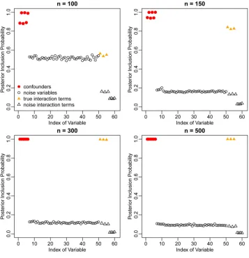
Figure 2 shows the PIPs assigned by BAC to the 50 potential confounders as well as the 10 potential interactions. High PIPs are given to true confounders (V1 to V6, red dots) and true

interactions (X with V1, V3, and V5, yellow filled triangles), indicating that BAC is able to

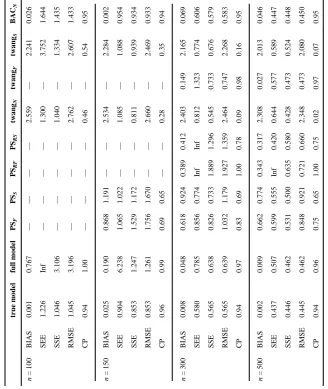
identify both true confounders and true interactions, with higher PIPs for the larger sample sizes. For this scenario, we compare the estimate of ACE from BACN to the stratification by

propensity score method (PSF, PSS, PSRF, and PSRS), the twang method (twangN, twangF,

and twangS), the true model, and the full model. Results are summarized in Table 2. BACN

performs well for all sample sizes, and stabilization with an informative prior is not required. The CP is very close to the desired value. In contrast, estimates from most propensity score methods are either largely biased or unstable. The only propensity score method that appears to have small bias is twangF, but this method fails to provide reliable

results for n = 100 or 150 and has RMSE larger than BACN for n = 300 or 500.

Author Manuscript

(12)

Web appendix E uses standardized bias (B) values (Rubin, 2007) to illustrate the difficulty in using the estimated propensity score to balance covariates when there are a lot of potential confounders and limited number of observations. Web appendices H, I, and J provide additional simulations to illustrate BAC in situations a) with both binary and continuous confounders that are correlated; b) with an alternative prior that permits interaction terms without main effects; and c) when the outcome model is misspecified. In all three situations, BAC reliably estimates the ACE and performs comparably to the comparison methods. Web appendix K compares BAC against the high dimensional propensity score approach of Schneeweiss et al. (2009). BAC provides improved performance relative to that method.

4. Evaluating the Causal Effect of Surgery on Thirty-day Readmission Rate

for Brain Tumor Patients

Thirty-day hospital readmission is one of the most important pay-for-performance bench- marks and is used by policy makers as an indicator of hospital quality (Nuño et al., 2014). We use Medicare data from 15060 brain tumor patients diagnosed between 2000 and 2009 in the US to assess whether surgical removal of the tumor reduces thirty-day readmission rate. Here, the time-to-readmission is calculated from the discharge date of the

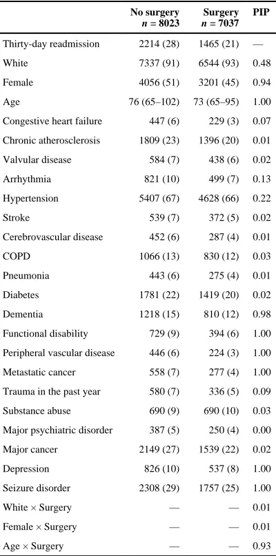
hospitalization when the cancer was diagnosed to the time of re-hospitalization. Patients who died within a month after diagnosis are excluded from the analysis (Nuño et al., 2014). We consider a set of 23 potential confounders listed in Table 3.

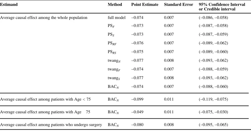
We apply the BAC method based on logistic regression models. The full model includes surgery, the 23 potential confounders as well as interactions between surgery and demographic characteristics including age, gender and race. For comparison, we also consider the full model, the stratification on propensity score method (PS_F, PS_S, PS_RF, and PS_RS) and the twang method (twang_N, twang_F, and twang_S). All the methods yield very similar ACE estimates, indicating a statistically significant effect of surgery in reducing thirty-day readmission rate (Table 4). We also calculate the PIPs for potential confounders and interaction terms (Table 3). The interaction between surgery and age has a very high PIP equal to 0.93, evidencing a heterogeneous causal effect in patients with different ages. The TEH is also indicated by propensity score stratification, with stratum-specific ACE estimates indicating a stronger effect for higher levels of the propensity score (see Web Table 4). The lowest quintile exhibits an ACE of −0.026 (95% CI −0.059, 0.006), while the highest quintile has an ACE of −0.115 (95% CI −0.147, −0.083). While differences in ACE for different propensity score strata do not directly provide interpretable evidence about which patients exhibit TEH, the fact that average age decreases in the five propensity score strata (Web Table 4) suggests that the surgery effect may differ in patients with different ages. Thus, in this context, the presence of TEH is evident by estimating effects that differ across propensity score strata, and post-hoc investigation suggests that this heterogeneity is driven by age.

To further investigate TEH, we use BAC to estimate the average causal effects for patients less than 75 years old and greater than 75 years old separately. This procedure uses the same model posteriors obtained from the entire population, but only V values from patients from a given age group in equation (A1) in the Web Appendix. The average causal effect of surgery

Author Manuscript

(13)

for patients less than 75 years old is −0.099 (95 % CI −0.119, −0.075), which is much larger than that for patients greater than 75 years old (Table 4).

We also use BAC to estimate the average causal effect among patients who undergo surgery, known as the average causal effect for the treated (ATT) (Rubin, 1977; Imbens, 2004). The ATT reflects the treatment effect on those who ultimately receive the treatment. We again utilize the same model posteriors but plug in observed V values only from patients who had surgery in equation (A1). The estimated ATT (Table 4) is −0.080 (95% CI −0.095, −0.065).

To investigate small-sample performance of BAC in real data, we randomly sample 0.5% (n = 75), 1% (n = 150), or 2% (n = 300) patients from our data and apply BAC (BACN and

BACI), the full model, the stratification by propensity score method (PSF, PSS, PSRF, and

PSRS) and the twang method (twangN, twangF, and twangS) to estimate ACE. Results from

500 replicates are listed in Web Table 5, where the ACE estimate from the whole data set is considered as the “true” value for each method. For the case n = 150, the RMSEs from BACN and BACI are at least 10% and 20% smaller than those from all the variations of the

stratification by propensity score method, respectively. The results from BAC are

comparable to those from the twang method (twangN, twangF, and twangS). For the case n =

75, both the stratification by propensity score method (PSF, PSS, PSRF, and PSRS) and

BACN fail to provide usable estimates, similar to what we observed in Section 3. But BACI

and the twang method can still provide a usable estimate of the ACE, with the RMSE from BACI at least 15% smaller than those from all the variations of the twang method.

5. Discussion

We present a general framework to adjust for confounders with explicit consideration of interactions between confounders and exposure. We propose an automatic and data-driven procedure that accounts for uncertainty in which confounders and effect modifiers should be considered by jointly modeling exposure and outcome models. While our illustrations present binary or count data, the method can also be applied to any data type within the GLM framework. Computation with the MC3 algorithm (Madigan et al., 1995) is appealing for its simplicity in high dimensional settings, but other approaches to Bayesian variable selection such as the hierarchical mixture prior of George and McCulloch (1993) could also be adapted to the task considered here, possibly at the cost of increased computational burden. Note that the parametric models considered here can be easily relaxed by considering smooth non-linear functions in outcome or exposure models.

BAC can be used to estimate the average causal effect not only for the whole population but also for any subpopulation of interest. All the estimates are then still based on equation (6) with the same p(αY_{|D) on the model space, estimated by using all observed data. The}

difference lies in the specification and estimation of θ, which represents the distribution of V. To estimate θ for a given subpopulation, one needs to plug in observed data only from that subpopulation into equation (A1). Our procedure maximizes the utilization of all observed data to build models in the estimation of the ACE for a subpopulation. Because there is no data discarding, our method is likely to achieve a higher efficiency (Little et al.,

Author Manuscript

(14)

2000). The independence of the posteriors of θ and βαY allows estimation of causal effects in subpopulations by simply re-generating samples of θ according to that subpopulation. One limitation of BAC is that it provides no immediate way to check for balance or overlap in the empirical distributions of confounders in exposed and nonexposed groups. This is in contrast to propensity score methods that permit the checking based on estimated propensity scores (Rubin, 2007). Without confirming covariate balance and overlap, causal inference with BAC may be subject to model-based extrapolation. BAC is particularly well suited to settings where high dimensional covariate information compromises the ability to check for balance and overlap, for example, because the propensity score cannot be estimated reliably or because there are simply too many covariate dimensions to check. A virtue of BAC in these contexts is that it concentrates posterior support on models that only include the most relevant confounders (and interaction terms) for estimating the ACE. This provides some protection against unnecessarily separating covariate distributions on the basis of factors that are extraneous with respect to ACE estimation (Schafer and Kang, 2008). With knowledge of PIPs, overlap checking can focus on only the most relevant factors, for example, by combining PIPs with overlap checking methods such as the convex hull method (King and Zeng, 2006).

BAC provides an automatic and transparent way to indicate interactions between potential confounders and the treatment. While the methods developed here limit consideration to two-way interactions between a single covariate and treatment, extensions to include higher-order interaction terms in (2) could help identify complex groups of variables that modify treatment effects. Inclusion of a limited number of higher-order interactions that are of suspected importance a priori is straightforward. However, novel methods would be required to enable efficient selection of the potentially huge number of possible higher-order interaction terms. Nonetheless, the ability to aid scientific interpretability by identifying the specific factors that interact with the treatment is an important feature of BAC, and another point of contrast with propensity scores. While propensity score analyses can provide evidence of TEH on the basis of the propensity score, such analyses will not necessarily provide information about the specific, interpretable factors that define types of patients exhibiting different effects. Knowledge that patients with different propensity scores experience different effects is not likely to provide any clinically meaningful value. While post-hoc analyses of how individual factors vary with values of the propensity score may possibly identify factors that drive TEH, as was the case with age in our analysis of surgery for brain cancer patients, systematic approaches to automatically identify such factors and to incorporate such information in the ACE estimation are unavailable. This limits the use of propensity scores for characterizing TEH in any scientifically or clinically interpretable manner, especially when the factors that might drive TEH are high dimensional.

In this paper, we choose the dependence parameter ω in equation (7) to be infinity, which, conditional on αX_{, forces predictors of exposure to be included in the outcome model. In}

practice, we suggest investigators to choose ω based on the design of their study and their knowledge about the data. If investigators are confident in excluding instrumental variables that are associated with X but not Y prior to the analysis, choosing ω = ∞ is optimal. However, if there is uncertainty about the presence of such variables, choosing ω = ∞ may

Author Manuscript

(15)

reduce the efficiency of the ACE estimation (Brookhart et al., 2006; Schafer and Kang, 2008; Wang et al., 2012). Under such situation, we suggest investigators to choose a finite

ω, as we pointed out in our previous publication (Wang et al., 2012). Investigators may also consider a more automatic procedure for choosing ω, which was proposed by Lefebvre et al. (2014).

The purpose of our analysis for estimating the ACE of surgery on the thirty-day readmission rate in brain tumor patients is to illustrate the use of BAC in real data. Because there were 13.8% of patients who died within a month and our analysis excluded those patients, the ACE estimation may be subject to selection bias. A more appropriate approach is to consider the time-to-readmission as the outcome variable. Extending BAC to deal with censored data and time-to-event outcomes is one of our future research.

Supplementary Material

Refer to Web version on PubMed Central for supplementary material.

Acknowledgments

We thank Dr. Nils Arvold and Dr. Yun Wang for input on the construction and analysis of the brain cancer data. We also thank the Co-Editor, the Associate Editor, and three referees for insightful comments. The work of Drs. Dominici and Zilger was supported by NIH/NCI P01 CA134294, and HEI 4909, and Dr. Dominici was supported by AHRQ K18 HS021991.

References

Brookhart MA, Schneeweiss S, Rothman KJ, Glynn RJ, Avorn J, Stürmer T. Variable selection for propensity score models. American Journal of Epidemiology. 2006; 163:1149–1156. [PubMed: 16624967]

George EI, McCulloch RE. Variable selection via gibbs sampling. Journal of the American Statistical Association. 1993; 88:881–889.

Greenland S, Robins JM, Pearl J. Confounding and collapsibility in causal inference. Statistical Science. 1999; 14:29–46.

Imai K, Van Dyk DA. Causal inference with general treatment regimes. Journal of the American Statistical Association. 2004; 99:854–866.

Imbens GW. Nonparametric estimation of average treatment effects under exogeneity: A review. Review of Economics and Statistics. 2004; 86:4–29.

King G, Zeng L. The dangers of extreme counterfactuals. Political Analysis. 2006; 14:131–159. Kurth T, Walker AM, Glynn RJ, Chan KA, Gaziano JM, Berger K, Robins JM. Results of

multivariable logistic regression, propensity matching, propensity adjustment, and propensity-based weighting under conditions of nonuniform effect. American Journal of Epidemiology. 2006; 163:262–270. [PubMed: 16371515]

Lefebvre G, Delaney JA, McClelland RL. Extending the Bayesian adjustment for confounding algorithm to binary treatment covariates to estimate the effect of smoking on carotid intima-media thickness: the multi-ethnic study of atherosclerosis. Statistics in Medicine. 2014; 33:2797–2813. [PubMed: 24596278]

Little RJ, An H, Johanns J, Giordani B. A comparison of subset selection and analysis of covariance for the adjustment of confounders. Psychological Methods. 2000; 5:459. [PubMed: 11194208] Lunceford JK, Davidian M. Stratification and weighting via the propensity score in estimation of

causal treatment effects: a comparative study. Statistics in Medicine. 2004; 23:2937–2960. [PubMed: 15351954]

Author Manuscript

(16)

Lunt M, Solomon D, Rothman K, Glynn R, Hyrich K, Symmons DP, Stürmer T, et al. Different methods of balancing covariates leading to different effect estimates in the presence of effect modification. American Journal of Epidemiology. 2009; 169:909–917. [PubMed: 19153216] Madigan D, York J, Allard D. Bayesian graphical models for discrete data. International Statistical

Review/Revue Internationale de Statistique. 1995; 63:215–232.

McCandless LC, Gustafson P, Austin PC. Bayesian propensity score analysis for observational data. Statistics in Medicine. 2009; 28:94–112. [PubMed: 19012268]

Newton MA, Raftery AE. Approximate Bayesian inference with the weighted likelihood bootstrap. Journal of the Royal Statistical Society. Series B (Methodological). 1994; 56:3–48.

Nuño M, Ly D, Ortega A, Sarmiento JM, Mukherjee D, Black KL, Patil CG. Does 30-day readmission affect long-term outcome among glioblastoma patients? Neurosurgery. 2014; 74:196–205. [PubMed: 24176955]

Raftery AE, Madigan D, Hoeting JA. Bayesian model averaging for linear regression models. Journal of the American Statistical Association. 1997; 92:179–191.

Ridgeway, G.; McCaffrey, D.; Morral, A.; Burgette, L.; Griffin, BA. R Vignette. RAND; 2014. Toolkit for weighting and analysis of nonequivalent groups: A tutorial for the twang package. Rosenbaum PR, Rubin DB. The central role of the propensity score in observational studies for causal

effects. Biometrika. 1983; 70:41–55.

Rubin DB. Estimating causal effects of treatments in randomized and nonrandomized studies. Journal of Educational Psychology. 1974; 66:688–701.

Rubin DB. Assignment to treatment group on the basis of a covariate. Journal of Educational and Behavioral Statistics. 1977; 2:1–26.

Rubin DB. The Bayesian bootstrap. The Annals of Statistics. 1981; 9:130–134.

Rubin DB. The design versus the analysis of observational studies for causal effects: parallels with the design of randomized trials. Statistics in Medicine. 2007; 26:20–36. [PubMed: 17072897] Schafer JL, Kang J. Average causal effects from nonrandomized studies: a practical guide and

simulated example. Psychological Methods. 2008; 13:279. [PubMed: 19071996] Schneeweiss S, Rassen JA, Glynn RJ, Avorn J, Mogun H, Brookhart MA. High-dimensional

propensity score adjustment in studies of treatment effects using health care claims data. Epidemiology (Cambridge, Mass). 2009; 20:512.

Vansteelandt, S. Discussions on “Bayesian effect estimation accounting for adjustment uncertainty”. In: Wang, C.; Parmigiani, G.; Dominici, F., editors. Biometrics. Vol. 68. 2012. p. 675-678. Wang C, Parmigiani G, Dominici F. Bayesian effect estimation accounting for adjustment uncertainty.

Biometrics. 2012; 68:661–671. [PubMed: 22364439]

Zigler CM, Dominici F. Uncertainty in propensity score estimation: Bayesian methods for variable selection and model-averaged causal effects. Journal of the American Statistical Association. 2014; 109:95–107. [PubMed: 24696528]

Author Manuscript

(17)

[image:17.612.119.555.61.509.2]

Figure 1.

Marginal posterior inclusion probabilities of the 50 potential Mconfounders in the first simulation scenario, based on BAC.

Author Manuscript

(18)

[image:18.612.158.515.63.434.2]

Figure 2.

Marginal posterior inclusion probabilities of the 50 potential confounders and 10 potential interaction terms in the second simulation scenario, based on BAC.

Author Manuscript

(19)

Author Manuscript

[image:19.612.93.419.196.679.2]

Author Manuscript

Table 1

Estimation of ACE in the first simulation scenario.

true model full model Ad hoc 1 Ad hoc 5 PS F PS S PS RF PS RS twang N twang F twang S BAC N BAC I n = 100 BIAS 0.003 0.044 0.036 0.019 — — — — 0.036 0.008 0.063 — 0.009 SEE 0.110 0.264 0.245 0.172 — — — — 0.102 0.109 0.107 — 0.078 SSE 0.104 0.223 0.213 0.191 — — — — 0.081 0.091 0.103 — 0.079 RMSE 0.104 0.227 0.216 0.191 — — — — 0.088 0.092 0.121 — 0.080 CP 0.95 1.00 1.00 0.94 — — — — 0.97 1.00 0.91 — 0.95 n = 150 BIAS 0.000 0.023 0.036 0.053 0.027 0.028 0.008 0.019 0.037 0.004 0.061 0.015 0.010 SEE 0.084 0.198 0.185 0.156 0.094 0.091 0.203 0.099 0.085 0.089 0.086 0.081 0.075 SSE 0.079 0.126 0.137 0.148 0.141 0.124 0.206 0.140 0.066 0.082 0.077 0.081 0.068 RMSE 0.079 0.128 0.142 0.157 0.143 0.127 0.206 0.141 0.076 0.082 0.098 0.082 0.068 CP 0.96 1.00 0.96 0.92 0.77 0.82 0.94 0.82 0.95 1.00 0.89 0.94 0.97 n = 300 BIAS 0.001 0.000 0.009 0.018 0.009 0.017 0.006 0.023 0.035 0.001 0.049 0.005 0.004 SEE 0.058 0.070 0.082 0.091 0.071 0.068 0.191 0.072 0.063 0.065 0.061 0.058 0.057 SSE 0.058 0.065 0.074 0.077 0.072 0.068 0.132 0.107 0.047 0.065 0.062 0.059 0.055 RMSE 0.058 0.065 0.074 0.079 0.073 0.070 0.133 0.109 0.058 0.065 0.079 0.060 0.055 CP 0.95 0.95 0.95 0.93 0.93 0.95 1.00 0.79 0.97 0.99 0.85 0.95 0.95 n = 500 BIAS 0.001 0.001 0.007 0.013 0.012 0.016 0.039 0.042 0.033 0.001 0.038 0.002 0.002 SEE 0.044 0.047 0.053 0.058 0.052 0.050 0.120 0.068 0.051 0.047 0.047 0.045 0.044 SSE 0.043 0.046 0.050 0.053 0.049 0.048 0.100 0.096 0.036 0.046 0.047 0.043 0.042 RMSE 0.043 0.046 0.051 0.055 0.051 0.050 0.107 0.104 0.049 0.046 0.060 0.043 0.042 CP 0.95 0.97 0.97 0.96 0.96 0.95 0.98 0.78 0.97 0.97 0.87 0.96 0.96

(20)

Author Manuscript

[image:20.612.91.419.292.681.2]

Author Manuscript

Table 2

Estimation of ACE in the second simulation scenario.

true model full model PS F PS S PS RF PS RS twang N twang F twang S BAC N n = 100 BIAS 0.001 0.767 — — — — 2.559 — 2.241 0.026 SEE 1.226 Inf — — — — 1.300 — 3.752 1.644 SSE 1.046 3.106 — — — — 1.040 — 1.334 1.435 RMSE 1.045 3.196 — — — — 2.762 — 2.607 1.433 CP 0.94 1.00 — — — — 0.46 — 0.54 0.95 n = 150 BIAS 0.025 0.190 0.868 1.191 — — 2.534 — 2.284 0.002 SEE 0.904 6.238 1.065 1.022 — — 1.085 — 1.088 0.954 SSE 0.853 1.247 1.529 1.172 — — 0.811 — 0.939 0.934 RMSE 0.853 1.261 1.756 1.670 — — 2.660 — 2.469 0.933 CP 0.96 0.99 0.69 0.65 — — 0.28 — 0.35 0.94 n = 300 BIAS 0.008 0.048 0.618 0.924 0.389 0.412 2.403 0.149 2.165 0.069 SEE 0.580 0.785 0.856 0.774 Inf Inf 0.812 1.323 0.774 0.606 SSE 0.565 0.638 0.826 0.733 1.889 1.296 0.545 0.733 0.676 0.579 RMSE 0.565 0.639 1.032 1.179 1.927 1.359 2.464 0.747 2.268 0.583 CP 0.94 0.97 0.83 0.69 1.00 0.78 0.09 0.98 0.16 0.95 n = 500 BIAS 0.002 0.009 0.662 0.774 0.343 0.317 2.308 0.027 2.013 0.046 SEE 0.437 0.507 0.599 0.555 Inf 0.420 0.644 0.577 0.589 0.447 SSE 0.446 0.462 0.531 0.500 0.635 0.580 0.428 0.473 0.524 0.448 RMSE 0.445 0.462 0.848 0.921 0.721 0.660 2.348 0.473 2.080 0.450 CP 0.94 0.96 0.75 0.65 1.00 0.75 0.02 0.97 0.07 0.95

(21)

Author Manuscript

[image:21.612.81.281.133.536.2]

Author Manuscript

Table 3

Patients’ characteristics and posterior inclusion probabilities (PIPs) from BAC. Data from Medicare Part A for the period between 2000 and 2009

No surgery n = 8023

Surgery n = 7037

PIP

Thirty-day readmission 2214 (28) 1465 (21) —

White 7337 (91) 6544 (93) 0.48

Female 4056 (51) 3201 (45) 0.94

Age 76 (65–102) 73 (65–95) 1.00

Congestive heart failure 447 (6) 229 (3) 0.07

Chronic atherosclerosis 1809 (23) 1396 (20) 0.01

Valvular disease 584 (7) 438 (6) 0.02

Arrhythmia 821 (10) 499 (7) 0.13

Hypertension 5407 (67) 4628 (66) 0.22

Stroke 539 (7) 372 (5) 0.02

Cerebrovascular disease 452 (6) 287 (4) 0.01

COPD 1066 (13) 830 (12) 0.03

Pneumonia 443 (6) 275 (4) 0.01

Diabetes 1781 (22) 1419 (20) 0.02

Dementia 1218 (15) 810 (12) 0.98

Functional disability 729 (9) 394 (6) 1.00

Peripheral vascular disease 446 (6) 224 (3) 1.00

Metastatic cancer 558 (7) 277 (4) 1.00

Trauma in the past year 580 (7) 336 (5) 0.09

Substance abuse 690 (9) 690 (10) 0.03

Major psychiatric disorder 387 (5) 250 (4) 0.00

Major cancer 2149 (27) 1539 (22) 0.02

Depression 826 (10) 537 (8) 1.00

Seizure disorder 2308 (29) 1757 (25) 1.00

White × Surgery — — 0.01

Female × Surgery — — 0.01

Age × Surgery — — 0.93

(22)

Author Manuscript

[image:22.612.83.521.120.349.2]

Author Manuscript

Table 4

mission rate for brain tumor patients

Estimand Method Point Estimate Standard Error 95% Confidence Interval

or Credible interval

Average causal effect among the whole population full model −0.074 0.007 (−0.086, −0.058)

PSF −0.073 0.007 (−0.087, −0.058)

PSS −0.073 0.007 (−0.087, −0.059)

PSRF −0.076 0.007 (−0.089, −0.062)

PSRS −0.075 0.007 (−0.089, −0.060)

twangN −0.077 0.008 (−0.093, −0.062)

twangF −0.074 0.007 (−0.088, −0.059)

twangS −0.077 0.008 (−0.093, −0.062)

BACN −0.074 0.007 (−0.088, −0.060)

Average causal effect among patients with Age < 75 BACN −0.099 0.011 (−0.119, −0.075)

Average causal effect among patients with Age ≥ 75 BACN −0.049 0.011 (−0.075, −0.030)