An in-depth numerical study of the two-dimensional Kuramoto–Sivashinsky equation

(1)

This is a repository copy of

An in-depth numerical study of the two-dimensional

Kuramoto–Sivashinsky equation

.

White Rose Research Online URL for this paper:

http://eprints.whiterose.ac.uk/88551/

Version: Accepted Version

Article:

Kalogirou, A, Keaveny, EE and Papageorgiou, DT (2015) An in-depth numerical study of

the two-dimensional Kuramoto–Sivashinsky equation. Proceeding of the Royal Society A,

471 (2179). ISSN 1364-5021

https://doi.org/10.1098/rspa.2014.0932

[email protected]

https://eprints.whiterose.ac.uk/

Reuse

Unless indicated otherwise, fulltext items are protected by copyright with all rights reserved. The copyright

exception in section 29 of the Copyright, Designs and Patents Act 1988 allows the making of a single copy

solely for the purpose of non-commercial research or private study within the limits of fair dealing. The

publisher or other rights-holder may allow further reproduction and re-use of this version - refer to the White

Rose Research Online record for this item. Where records identify the publisher as the copyright holder,

users can verify any specific terms of use on the publisher’s website.

Takedown

If you consider content in White Rose Research Online to be in breach of UK law, please notify us by

(2)

2

rspa.ro

y

alsocietypub

lishing.org

Proc

R

Soc

A

0000000

..

1. Introduction

The one-dimensional Kuramoto-Sivashinsky equation (KSE)

ut+uux+uxx+uxxxx= 0, (1.1a)

u(x, t) =u(x+ 2L, t), u(x,0) =u0(x), (1.1b)

where0≤x <2Lis the spatial coordinate andtis time; solutions are sought on spatially periodic domains of size2L, andu0(x)is the initial condition. The KSE is one of the simplest nonlinear PDEs exhibiting complex spatio-temporal dynamics. It was derived by both Homsy [1] and Nepomnyashchii [2] in their studies of thin liquid film flows down inclined planes, by LaQueyet al.[3] in trapped ion mode instabilities, by Kuramoto [4] in diffusion-induced chaos in reaction systems, and Sivashinsky and collaborators [5–7] in their studies of flame front propagation. It has since been found to describe the asymptotic behaviour of other physical phenomena, including two–phase flows in cylindrical pipes [8], interfacial flows [10,11], plasma and chemical reaction dynamics [4,12,13], and models of ion-sputtered surfaces [14] that extend the equation to higher dimensions also. Note that (1.1) is equivalent (in one dimension) to the integrated form

vt+1

2v

2

x+vxx+vxxxx= 0, (1.2)

through the transformationu=vx. Flame propagation applications are usually governed by the integrated form (1.2) whereas fluid film flows are governed by the conservative form (1.1).

In addition to its intrinsic physical relevance, the 1D KSE has attracted significant mathematical interest, becoming a premier model for studying complex dynamics in spatially extended systems. There have been numerous analytical [15–19] and numerical [20–23] studies of the 1D KSE with 2L−periodic boundary conditions (see below also). The 1D KSE has been proven to possess a unique smooth solution that depends continuously on its initial data [19]. Its convective Burgers–type nonlinearity provides a transfer of energy between active and dissipative modes, and the essence of the dynamics can be captured by a finite dimensional dynamical system of ordinary differential equations for the Fourier coefficients of the solution.

A significant portion of the analytical work on the 1D KSE has focused on how the energy

(defined as the L2−norm of the solution, kukL2:=

_R₂_L

0 u

2₍_{x, t}₎_dx1/2

) scales with domain length. Assuming that the domain is finite (L <∞; ifL=∞the PDE is ill-posed), long–time solutions are bounded by an absorbing ball with an L−dependent radius (inL2 and higher Sobolev spaces) such that

lim sup

t→∞

kukL2=O L

p_.

(1.3)

The first value ofpobtained wasp= 5/2for odd–parity solutions [18], though this estimate has been improved over the years by many mathematicians [15,17,24–28]. The current best known analytic bound iso(L3/2)[26,28], though the numerical study by Whittenberg & Holmes [29] has suggested the optimal valuep= 1/2.

(3)

3

rspa.ro

y

alsocietypub

lishing.org

Proc

R

Soc

A

0000000

..

are extensive in that the local dynamics are asymptotically independent ofLforL≫1and the energy is equally distributed amongst the lowest Fourier modes [29].

Despite the rich dynamics established for the 1D KSE, studies in higher dimensions are somewhat limited and primarily analytical. The spatially periodic 2D KSE is

ut+1

2|∇u|

2₊_∆u₊_∆2_u_{= 0}_,

(1.4)

u(x, y;t) =u(x+ 2Lx, y;t) =u(x, y+ 2Ly, t), u(x, y,0) =u0(x, y), (1.5)

where ∆=∂2x+∂y2. It has been established by Cao & Titi [33] that the only locally integrable stationary solutions of the 2D KSE (on infinite domains) are constant values, but the question of global regularity for the KSE in higher dimensions is still an open problem in nonlinear analysis. The first attempts at proving boundedness, analyticity, and stability for the 2D KSE were by Sell & Taboada [34] and Molinet [35]. Assuming a thin domain, [34] showed the existence of a bounded absorbing set inHper1 ([0,2π]×[0,2πǫ])forǫsufficiently small. Molinet [35] improved this result showing that with some restrictions on the initial data,

lim sup

t→∞

kukL2≤ O

L8x/5L1y/2

, (1.6)

on the bounded domain(0,2Lx)×(0,2Ly)with2Lx≥2π,0<2Ly<2πsatisfying

1−(Ly/2π)2

₋4 9

Ly≤CL−x67/35. (1.7)

For radially symmetric solutions, Demirkaya & Stanislavova [36] proved that there exists a time independent bound for theL2–norm of the solution, while Michelson [37] showed the existence of a nontrivial radial steady solution that is asymptotically periodic. Other authors have considered variants of the 2D KSE, mostly taking the form

ut+1

2

u2x+αu2y

+ (uxx+βuyy) +∆2u= 0, (1.8)

subject to boundary and initial conditions (1.5), though other variants have also been studied [38]. In (1.8),αandβare real parameters controlling the anisotropy of the nonlinear and linear terms, respectively. This anisotropic equation was derived by Cuerno & Barabáci [14] to describe the nonlinear evolution of surfaces eroded by ion bombardment. It was also studied by Rost & Krug [39] for different combinations of the signs ofαandβ. Forα=β >0andO(1), the solutions are bounded and develop into travelling waves that can become oscillatory or chaotic.

In this paper, we provide a comprehensive numerical study of the 2D KSE to complement (and possibly guide) the emerging body of analytical work on this equation. The combination of numerical and analytical studies of the 1D KSE has provided a deep understanding of its solutions and the physical phenomena it describes. It is our goal to extend this tandem approach to the 2D KSE. While there have been a number of numerical studies dedicated to the damped 2D KSE (see for example [40,41] and references therein), a complete numerical study of the 2D KSE (1.4) has not been performed, to the best of our knowledge. In what follows, we study in detail how the solution varies with the domain size by identifying the different attractors and describing their characteristics. We find that many results from the 1D case apply to the 2D equation also, but many others, including the hierarchy of bifurcations, are quite different. In addition, we study the energy of the solution in the chaotic regime. We examine both the dependence of the energy on system size and the dependence of the energy spectrum on wavenumber. We show that equipartition of energy holds in the chaotic regime for the differentiated version of the 2D KSE (see equation (2.4) below). We also find that the energy spectrum is radially symmetric in Fourier space and link this property to thex−ysymmetry of the equation.

(4)

4

rspa.ro

y

alsocietypub

lishing.org

Proc

R

Soc

A

0000000

..

of domain lengths in Section5. Finally, the main results and findings of this study are summarised in Section6.

2. Initial value problem and numerical methods

Throughout this study, we will be considering the initial value problem for the two–dimensional Kuramoto–Sivashinsky equation (1.4) on2Lx×2Ly−periodic domains as given by given by (1.5). We note that the mean

¯

u(t) = 1 4LxLy

Z2Lx

0

Z2Ly

0

u(x, y, t)dxdy (2.1)

of the solution is non-zero and grows in time according to

d

dtu¯(t) =−

1 8LxLy

Z2Lx

0

Z2Ly

0 |∇

u|2dxdy. (2.2)

To focus on the dynamics of the spatially varying part of the solution, we subtract off the growing mean value in our simulations (this is possible sinceu¯(t)does not contribute to the dynamics of the higher modes). Therefore, we consider the following mean–zero equation

vt+1

2 |∇v|

2 −₄_L1

xLy Z2Lx

0

Z2Ly

0 |∇

v|2dxdy

!

+∆v+∆2v= 0 (2.3)

forv(x, y, t) =u(x, y, t)−¯u(t), subject to the same periodic boundary conditions (1.5). The mean can also be removed by differentiating (1.4) with respect toxandyto obtain the system

U_t_{+ (}U_{· ∇}₎U₊_∆U₊_∆2U_{= 0} _(2.4)

of two mean–zero equations forU₌_∇_u_{. This approach has been adopted in many analytical}

studies [33–36], though for our computations we found using (2.3) to be more straightforward. With the mean removed, we solve (2.3) subject to the initial condition

v(x, y,0) = sin(πx/Lx+πy/Ly) + sin(πx/Lx) + sin(πy/Ly) (2.5)

using a Fourier pseudospectral method. This particular choice of initial condition is discussed in Section4. The spatial domain[0,2Lx]in thex−direction is split into2Mxequidistant points and similarly the domain in they−direction is discretised using2Mypoints. We express the solution as a Fourier series defined on these grid points and consider the system of ordinary differential equations for a finite number of Fourier modes. We compute the nonlinear terms on the grid using FFTs to go from Fourier to real space and back again. The time integration of the Fourier modes is carried out using a second–order accurate backwards difference scheme (BDF) that treats the linear terms implicitly. All codes are home-grown, written in Fortran 95 and compiled using an Intel Fortran compiler. For more details on these numerical methods see [42] for a related two-dimensional equation, and [43] for the dispersive 1D KSE.

In our simulations, we retainMx Fourier modes in thex-direction andMy modes in they -direction. For the most widely studied case whereLx=Ly=L, the number of Fourier modes

Mx=My=M depends onLor equivalentlyν=π2/L2 (see (4.4)). Forνbetween0.6and1.0,

M= 16 modes were found to provide sufficient resolution. For the smallest value ν= 0.005

(5)

5

rspa.ro

y

alsocietypub

lishing.org

Proc

R

Soc

A

0000000

..

0 2000 4000 6000 8000 10000

0 0.5 1 1.5 2 2.5 3 3.5

4x 10

5

L2

h

E

(

L

,

L

,

t

)

i

0 500 1000 1500

0 0.5 1 1.5 2 2.5x 10

5

LxLy

h

E

(

Lx

,

Ly

,

t

)

i

Ly= √

2π

Ly= 2π

[image:5.595.153.445.115.249.2]

(a)Lx=Ly=L. (b)Lyfixed.

Figure 1.Time–averaged energy versus domain area for (a)Case iand (b)Case iii. In panel (b), the crosses correspond

to the caseLy=√2πwhile the circles correspond toLy= 2π.

3. Chaos and Energy equipartition

We begin our study by exploring the statistical properties of the solution after it becomes chaotic. As shown later in Section4, the long-time solutions of the 2D KSE exhibit spatio–temporal chaos for large values of Lx,Ly. The rapid oscillations of these solutions suggest a universal bound for both space and time averages of the solutions [27]. We investigate the dependence of the time-averaged energy

hE(Lx, Ly, t)i= 1

T2−T1

ZT2

T1

Z2Lx

0

Z2Ly

0

v2(x, y, t)dxdydt (3.1)

on domain size asLx, Lybecome large. Here,h(·)i=_T2₋1T1

RT2

T1(·)dtdenotes time–average, and

the times0< T1< T2are large enough to ensure that the solution has entered the chaotic attractor. As discussed in [28], this quantity for the 1D KSE shares the same scaling with system sizeLas

lim supt_→∞kukL2, and so we adopt (3.1) in order to establish numerically the dependence ofLx

andLyonlim supt_→∞ku(·,·;t)kL2. In the computations described below the domain size is at

least as large as30×30. We also compute the average energy spectrum (i.e. the power spectrum)

S(k1, k2) = 4LxLy

D

|ˆv(k1, k2, t)|2

E = 1

T2−T1

ZT2

T1

4LxLy|vˆ(k1, k2, t)|2dt, (3.2)

which we normalise by including the factor4LxLy. By examining the power spectrum, we can understand how the energy is divided among different Fourier modes.

For the2L−periodic 1D KSE, numerical studies have shown that the time-averaged energy densityhE(L, t)i, whereE(L, t) =kvk2L2, is asymptotically proportional to the system sizeL[21,

29,44]. This suggests that the solution remainsO(1)and the energy density,L1hE(L, t)i, remains finite forL≫1. The numerically observed upper bound for theL2−norm is

lim sup

t_→∞ kvkL2≤cL 1/2

, (3.3)

while the best available analytic bound isOL5/6[28]. Wittenberg & Holmes [29] also show

that the time-averaged normalized energy spectrumS(k) = 2LD|vˆ(k, t)|2E, is independent ofk

(6)

6

rspa.ro

y

alsocietypub

lishing.org

Proc

R

Soc

A

0000000

..

Case i: L_x=L_y=LandL≫1

Here we solve the 2D KSE over square domains that increase in size. The time–averaged energyhE(L, L, t)iis plotted againstL2in Figure1(a) and shows a linear dependence. A least squares fit to the data data yields a resulting slope of approximately1.01so that

hE(L, L, t)i ∼const. L2, L≫1. (3.4)

Case ii: L_x= 10L_y= 10LandL≫1

This case is similar toCase i, but the domain is now a rectangle with aspect ratio10. Though not shown, we obtain a slope of about0.98by a least squares fit to the data. This suggests thathE(10L, L, t)i=OL2.

Case iii: L_yfixed,L_x≫1

Here the domain is a rectangle with fixed width2Ly=O(1)and increasing length2Lx. For two fixed values ofLy=√2π,2π, the time-averaged energy is plotted againstLxLy in Figure1(b). These values ofLyare chosen to ensure that there are unstable modes in they-direction (for largeLxthe domains are thin, but not as thin as the ones studied in [34] who had no unstable modes in they−direction). Least squares estimates of the slopes found them to be approximately1.01in both cases; hence, when one side of the domain is of fixed length and the other increases, the time-averaged energy scales with the dimension that is varied and produces the same scaling as the 1D KSE.

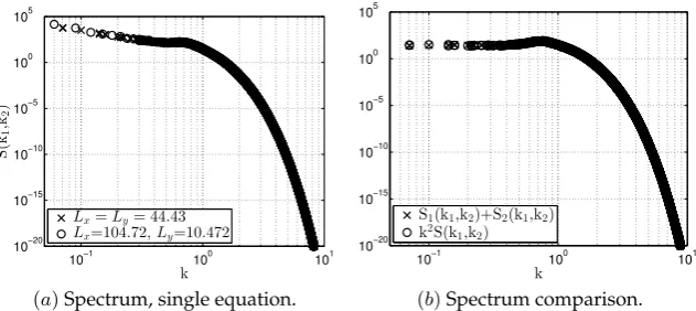
In addition to the energy, we characterise the average energy spectrum for domains chosen from Cases iandii. The values ofS(k1, k2)are shown in Figure2(a) against

k=qk2 1+k22=

s

n1π Lx

2

+

n2π Ly

2

, (3.5)

for two different sets of(Lx, Ly)(here the integers1≤n1≤Mxand1≤n2≤Myrepresent the Fourier modes of the two-dimensional solution). It can be seen that the average energy spectra for both sets of(Lx, Ly)have the same dependence onk. The independence of the average energy spectrum on domain size is also observed for the 1D KSE [45]. Fork≪1, we find thatS(k1, k2)∼ k−2_{, in contrast to a constant value found for the 1D KSE equation (}_1.1_{) in [}₂₉_{]. The factor of}

k−2_{, however, is due to the form of the nonlinearity in (}_2.3_{) rather than the dimensionality of the} problem. To see this, we note that (1.1) is not only (1.4) reduced to one dimension (i.e. equation (1.2)), but also differentiated with respect tox. The differentiation alters the form of the nonlinear term and yields the additional factor of|ik|2=k2to the energy spectrum. INote that thisk−2 dependence was observed by Yamada and Kuramoto [46] for the integrated equation (1.2).

Considering the differentiated system (2.4), we see that in Fourier space,

|Uc1k|2=|(vcx)_k|2=|ik1ˆvk|2=k21|ˆvk|2, |Uc2k|2=|(cvy)_k|2=|ik2ˆvk|2=k22|ˆvk|2 (3.6)

whereU1=vxandU2=vy. Adding these expressions together gives

|Uc1k|2+|Uc2k|2=

k21+k22

|vˆk|2=k2|vˆk|2. (3.7)

Figure2(b) showsk2S(k1, k2)alongside the sum of the two spectraS1(k1, k2) +S2(k1, k2)where Si(k1, k2) =

D

|cUik|2

E

. Here, we have taken the domain size to beLx=Ly=√π

0.005. The spectra coincide and the small differences can be attributed to statistical fluctuations in the data.

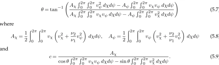
We further establish that the average energy spectrum for the 2D KSE is a function of the magnitude of the wavenumber,k=qk2₁+k2₂alone. This can be seen in Figures2and3(a). We note that this radial symmetry is present even if we haveLx6=Ly. To investigate this further, we consider (2.3) in Fourier space and multiply it byvˆ∗

k, the complex conjugate ofvˆk, to obtain

ˆ

v∗ k

(ˆvk)t+

1 2

\

|∇v|2 k−(k

2 −k4)ˆvk

(7)

7

rspa.ro

y

alsocietypub

lishing.org

Proc

R

Soc

A

0000000

..

10−1 100 101 10−20

10−15 10−10 10−5 100 105

k

S

(k1 ,k2

)

Lx=Ly= 44.43

Lx=104.72,Ly=10.472

10−1 100 101

10−20

10−15

10−10

10−5

100

105

k S1(k1,k2)+S2(k1,k2)

k2_S(k 1,k2)

[image:7.595.140.456.113.254.2]

(a)Spectrum, single equation. (b)Spectrum comparison.

Figure 2.Panel (a) shows the energy spectrumS(k1, k2), versuskforLx=Ly=π/√0.005(crosses), andLx=

10Ly=π/√0.0009 (circles). Panel (b) provides a comparison between k2S(k1, k2) (circles) and S1(k1, k2) +

S2(k1, k2)(crosses) forLx=Ly=π/√0.005.

where ˆc0(t) is real and denotes the (0,0) Fourier coefficient of the integral term 1

4LxLy

R2Lx

0

R2Ly

0 |∇v|2dxdy. Taking the complex conjugate of (3.8) yields

ˆ

vk

ˆ

v∗ k_t+

1 2

\

|∇v|2∗ k−(k

2

−k4)ˆv∗ k

= ˆc0(t). (3.9)

Adding (3.8) and (3.9) and averaging in time results in

d dt

D

|vˆk|2

E +Dˆv∗

k

\

|∇v|2 k+ ˆvk

\

|∇v|2∗ k

E

−2(k2−k4)D|vˆk|2

E

= 2hˆc0i. (3.10)

SincedD|vˆk|2

E

/dt= 0and the right hand side is independent ofk,D|vˆk|2

E

will be a function ofk

only ifDvˆ∗ k

\

|∇v|2 k+ ˆvk

\

|∇v|2∗ k

E

depends onkalone. As a consistency check, we calculated this term numerically and confirmed that indeed it depends only onk. This analysis suggests that the radial symmetry of the average energy spectrum is tied to the form of the nonlinearity of the 2D KSE, which is symmetric with respect toxandy. If we consider instead the following equation

vt+vvx+vxx+∆2v= 0 (3.11)

that arises in falling film applications [42,47–49] and lacks symmetry with respect toxandy, we find that its energy spectrum is not radially symmetric in(k1, k2)-space; for completeness this is shown in Figure3(b) where we have takenLx=Ly=√π

0.01.

4. Domain rescaling and linear stability

Before classifying how the solutions vary with domain size, we first rescale the spatial and time variables according to,

x→(Lx/π)x, y→(Ly/πy), t→(Lx/π)2t, (4.1)

in order to fix the domain size at[0,2π]×[0,2π]. The transformed equation is given by

ut+1

2|∇νu|

2₊_∆

νu+ν1∆2νu= 0, (4.2)

where

∇ν=

∂x,ν2

ν1∂y

, ∆ν=∂2x+

ν2 ν1∂

2

y, (4.3)

are the transformed operators and

(8)

8

rspa.ro

y

alsocietypub

lishing.org

Proc

R

Soc

A

0000000

..

[image:8.595.130.488.119.271.2]

(a)Symmetric 2D KSE (1.4). (b)Asymmetric equation (3.11).

Figure 3.Energy spectra from (a) the 2D KSE(2.3), and (b) the asymmetric equation(3.11)forLx=Ly=√π 0_.01.

are bifurcation parameters that play an important role in the dynamics. In rescaling space and time, information regarding the domain size has been transferred to these parameters which decrease asLxandLyincrease. The corresponding rescaled mean–zero equation forv(x, y, t) =

u(x, y, t)−u¯(t)is

vt+1

2 |∇νv|

2

− 1

4π2

Z2π

0

Z2π

0 |∇

νv|2dxdy

!

+∆νv+ν1∆2νv= 0. (4.5)

We assess the linear stability of the uniform statev= 0and establish the region of instability in(ν1, ν2)parameter space. Perturbing about the uniform statev= 0, a normal mode solution is sought in the form

v(x, y, t) =δei(n1x+n2y)+σt

+c.c., (4.6)

wheren1, n2are non–zero integer wavenumbers in thex−andy−directions respectively,δ≪1,σ is the complex amplification rate andc.c.denotes complex conjugates. Substituting (4.6) into (4.5) and linearising with respect toδ, results in the following dispersion relation

σ=

n21+ ν2 ν1n

2

2 1−ν1n21−ν2n22

(4.7)

that in turn implies the condition

ν1n21+ν2n22<1 (4.8)

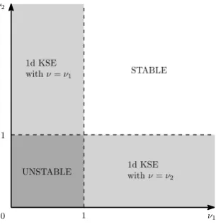
for instability. The inequality (4.8) can be satisfied for sufficiently smallν1,ν2(physically this is equivalent to large unscaled domains). By fixingν1andν2, we can determine the modes(n1, n2) for which the trivial solution is unstable, as summarised in Figure4. We see that forν1>1and ν2>1, (4.8) cannot be satisfied for anyn1, n2∈Z+and all sufficiently small perturbations from the trivial state decay to zero exponentially fast. Ifν1orν2is less than unity, instability sets in. For instance, if initiallyv(x, y,0) = sin(x+y)so thatn1= 1andn2= 1, a positive growth rate is ensured ifν1+ν2<1. A choice of an initial condition independent ofy, i.e.n2= 0, results in the instability condition being independent ofν2and yields the stability conditions for the 1D KSE (analogous results hold ifn1= 0). Based on the linear stability analysis, we take

v(x, y,0) = sin(x+y) + sin(x) + sin(y) (4.9)

(9)

9

rspa.ro

y

alsocietypub

lishing.org

Proc

R

Soc

A

0000000

..

1d KSE with_ν=_ν₂

ν1 ν2

STABLE

UNSTABLE 1d KSE with_ν=_ν₁

1 1

[image:9.595.221.374.110.269.2]

0

Figure 4.Stability diagram for the two–dimensional Kuramoto–Sivashinsky equation. The equation is stable when both

ν1, ν2>1. If eitherν1orν2is less than 1, then the dynamics are described by the 1D KSE. If bothν1, ν2<1then the solutions are fully two–dimensional.

5. Solutions and their dynamics

Using the numerical method described in Section 2, we solve the rescaled KSE (4.5) subject to the initial condition (4.9) for a range ofν1,ν2in the unstable region, namely0< ν1, ν2≤1(see Figure4). For the 1D KSE, steady state solutions arise for0.3< ν <1, approximately, whereν=

π L

2

, while smaller values ofνresult in travelling waves and time–periodic bursts [22,23]. When

ν≤0.12115, chaotic solutions appear via Feigenbaum subharmonic period–doubling bifurcations [22,23,30]. For the 2D KSE solutions also increase in complexity asν1, ν2→0, however, there are infinitely many routes to chaotic dynamics depending on the path in(ν1, ν2)space. We explore the path dependence in detail for two cases,ν1=ν2=νwithν→0, andν2→0withν1fixed.

We begin by performing numerical simulations over the unstable range ofν1andν2using step size∆ν= 0.05in each direction and classifying the solution at each(ν1, ν2)point. We exploit the symmetry of the 2D KSE aboutν1=ν2 (under a space and a time scale transformation) to reduce the number of simulations required: Ifv(x, y, t)is the solution corresponding to the values

(ν1, ν2), then the solution for(ν2, ν1)isv

y, x,ν2

ν1t

- this can be seen by multiplying the 2D KSE by ν1

ν2. We identify and study the different attractors by monitoring the energy of the solution

E(t) :=||v(·,·, t)||2L2=

Z2π

0

Z2π

0

v2(x, y, t)dxdy. (5.1)

This is related to the definition presented in (3.1) for2Lx×2Ly−periodic domains byE(t) =

√_ν

1√ν2E(Lx, Ly, t). We also consider

˙

E(t) = 2||vx||2+ 2ν2

ν1||vy|| 2

−2ν1||vxx||2−4ν2||vxy||2−2ν 2 2 ν1||vyy||

2 −

2_Zπ

0 2_Zπ

0 v

v2x+ν2

ν1v 2 y

dxdy,

(5.2) which we obtain by multiplying (4.5) byvand integrating over the periodic domain. Since the solution is periodic, quadratures are performed using the trapezoid rule to computeE(t) and

˙

E(t)to spectral accuracy; these values are in turn used to construct phase–planes (E(t),E˙(t)) which are particularly useful in identifying periodic and chaotic attractors. We also determine the Poincaré maps where E˙(t) = 0 in order to numerically generate return maps to describe the dynamics [22,23,30,43]. Using second–order polynomial interpolation, we find the timestn,

(10)

10

rspa.ro

y

alsocietypub

lishing.org

Proc

R

Soc

A

0000000

..

0

0.1

0.2

0.3

0.4

0.5

0.6

0.7

0.8

0.9

1

0

0.1

0.2

0.3

0.4

0.5

0.6

0.7

0.8

0.9

1

-6

ν1 ν2

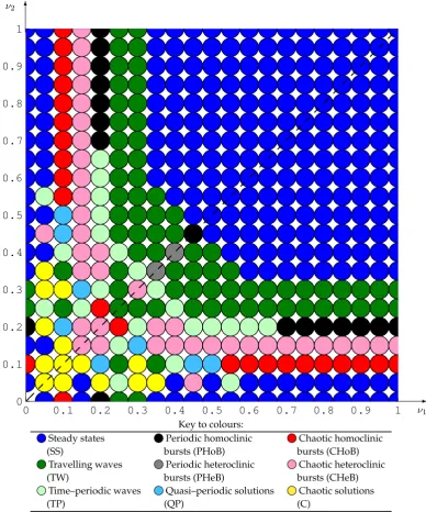
Key to colours:

Steady states Periodic homoclinic Chaotic homoclinic

(SS) bursts (PHoB) bursts (CHoB)

Travelling waves Periodic heteroclinic Chaotic heteroclinic

(TW) bursts (PHeB) bursts (CHeB)

Time–periodic waves Quasi–periodic solutions Chaotic solutions

[image:10.595.105.494.117.584.2]

(TP) (QP) (C)

Figure 5.Phase diagram classifying the solutions obtained for different values ofν1andν2for which the KSE is unstable.

about the attractor. If the return map contains just one point the solution is time–periodic with a single minimum in theE(t)signal (the period of oscillation can be estimated by calculating the time difference between two consecutive minima). If the return map contains continuous– looking curves that fill with points asnincreases, the solution is quasi–periodic, while foldings and self–similarity provide strong evidence for chaotic solutions [22,23,30,43,50].

(11)

11

rspa.ro

y

alsocietypub

lishing.org

Proc

R

Soc

A

0000000

..

C

TP

TW

C TW TW

CHeB SS PHeB PHoB SS

-ν

0 0.05 0.1 0.15 0.2 0.25 0.3 0.35 0.4 0.45

[image:11.595.108.480.119.188.2]

CHeB CHoB

Figure 6.Solutions obtained along the lineν1=ν2=νin parameter space. The solution abbreviations are given in the

caption of Figure5. The system size increases as we move to the left.

domain. As we decrease the values of ν1 and ν2, the steady state solutions are succeeded by travelling waves (TW) or time–periodic waves (TP), including periodic homoclinic bursts (PHoB) and periodic heteroclinic bursts (PHeB). For relatively small values ofν1,ν2, solutions characterised by quasi–periodic (QP) or chaotic (C) oscillations in time emerge. Chaotic solutions also appear in the form of chaotic homoclinic bursts (CHoB) or chaotic heteroclinic bursts (CHeB).

(a) Paths in

(

ν

1

, ν

2

)−

space

In this section a more detailed examination is undertaken to determine the dynamics along paths in(ν1, ν2)−space asν1, ν2→0. We first takeν1=ν2=νand compute solutions at equally spaced values ofνwith step size∆ν= 0.01. An outline of the most attracting solution types is given in the schematic diagram of Figure6(note that complexity emerges as we move from right to left). The first solutions to emerge are steady states for parameter values0.45≤ν <1. For0.43< ν <

0.45, the fixed point attractor overlaps with a time–periodic attractor, while for smaller values

0.35≤ν≤0.45, periodic heteroclinic bursts emerge as the time–periodic attractor competes with a new fixed point attractor. We see the first chaotic solutions for ν as high as 0.32. As we let

ν→0, the solutions alterate between travelling waves and chaotic dynamics untilν= 0.1, after which the solutions remain chaotic. This route to chaos was not found to follow the pattern of period doubling bifurcations found in the 1D KSE [22,23]. A notable characteristic of the chaotic solutions is that they retainO(1)amplitudes asνdecreases but the number of spatial oscillations increase. A similar result holds for the 1D KSE where it was proved that the number of rapid spatial oscillations increases linearly with the system size [32].

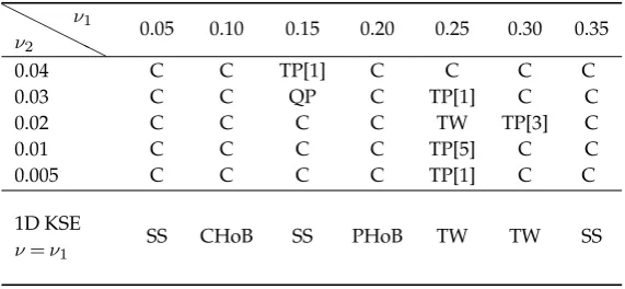
We also investigate the paths ν2→0 for small but fixedν1 between 0< ν1≤0.35. We are particularly interested in seeing whether the 1D KSE solutionsν=ν1are recovered in this limit

HH HH_H

ν2 ν1

0.05 0.10 0.15 0.20 0.25 0.30 0.35

0.04 C C TP[1] C C C C

0.03 C C QP C TP[1] C C

0.02 C C C C TW TP[3] C

0.01 C C C C TP[5] C C

0.005 C C C C TP[1] C C

1D KSE

ν=ν1 SS CHoB SS PHoB TW TW SS

Table 1.Solutions for0< ν1≤0.35andν2<0.05. For comparison, solutions to the 1D KSE for0< ν≤0.35are also

provided. Most abbreviations are given in the caption of Figure5. We use TP[m]to refer to a time–periodic solution with

[image:11.595.155.441.554.686.2]

(12)

12

rspa.ro

y

alsocietypub

lishing.org

Proc

R

Soc

A

0000000

..

2420 2440 2460 2480

2420 2430 2440 2450 2460 2470 2480

En

E

n

+

1

350 400 450 500 550 600

E_n

E

n

+

1

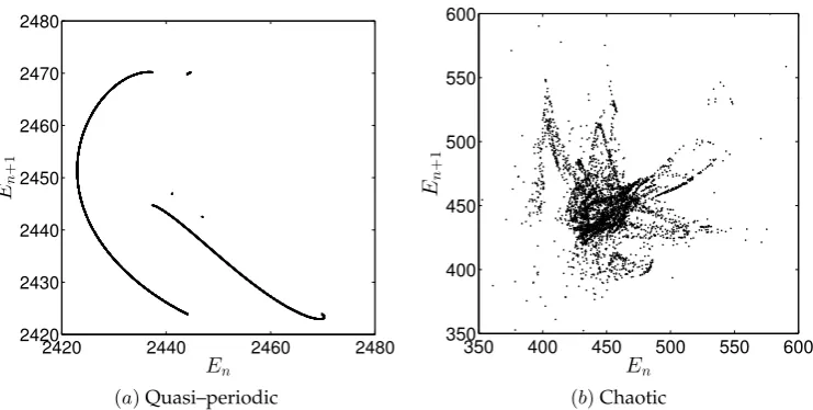
[image:12.595.114.485.112.299.2]

(a)Quasi–periodic (b)Chaotic

Figure 7.Return maps for (a) a quasi–periodic solution (ν1= 0.15,ν2= 0.03) and (b) a chaotic solution (ν1= 0.25,

ν2= 0.04)

- settingν2= 0in (4.2) can be seen to yield the 1D KSE withν=ν1. The results are summarised in Table1and it can be seen that asν2decreases, solutions are mostly chaotic. Interestingly, our computations do not reduce to the given solution type obtained from the 1D KSE for ν=ν1, thus suggesting that the limitν2→0is singular. In order to observe the quantitative nature of the attractors, two representative return maps are shown in Figure7. Panel (a) corresponds to a quasi–periodic solution obtained for(ν1, ν2) = (0.15,0.03)- quasi–periodicity is surmised by the continuous–looking curves. The return map for the solution obtained for(ν1, ν2) = (0.25,0.04)is illustrated in panel (b), which is surmised to be chaotic due to the presence of foliations.

It can also be seen from Figure5that steady states emerge whenν1andν2are relatively close to unity. In what follows we analyse asymptotically the bifurcated steady states emerging from these critical parameter values.

(b) Steady states

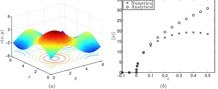
For ν1>1, ν2>1, solutions are attracted to the trivial statev= 0. At ν1=ν2= 1, a pitchfork bifurcation occurs and non–trivial solutions first appear. In a large region approximately enclosed by the lines ν1= 0.35, ν2= 0.35 and ν1+ν2= 0.95 (see Figure 5), the solutions are two-dimensional unimodal steady states with relatively low energy. A typical steady state for ν1= ν2= 0.9 is given in Figure8(a); it is fully twodimensional and unique up to a translation -equation (4.5) is translation invariant (we do not have a uniqueness proof - our statement is based on numerical experiments starting from arbitrary initial conditions). We can analyse solutions near the bifurcation point(ν1, ν2) = (1,1)by writing

ν1= 1−α1ǫ, ν2= 1−α2ǫ (5.3)

(13)

13

rspa.ro

y

alsocietypub

lishing.org

Proc

R

Soc

A

0000000

..

0 2

4 6

0 2 4 6 −6 −2 2 6

y x

v

(

x

,

y

)

−0.10 0 0.1 0.2 0.3 0.4 0.5

5 10 15 20 25 30 35

ǫ

||

v

||

Numerical Analytical

[image:13.595.113.487.118.271.2]

(a) (b)

Figure 8.(a) Steady state profile forν1=ν2= 0.9. (b) TheL2−normkvkof steady states for different values ofǫfor

the numerical (crosses) and analytical (circles) solutions. The analytical norm is found using(5.4)up to orderǫ1/2

.

from the transformationsU1=ux=vx,U2=uy=vy. The result is

v= 2(12ǫ)1/2hα1₁/2cos(x+φ1) +α1₂/2cos(y+φ2)

i

+ǫ[α1cos(2(x+φ1)) +α2cos(2(y+φ2))]

+ 4 ǫ 12

3/2h

α3₁/2cos(3(x+φ1)) +α32/2cos(3(y+φ2))

i

+Oǫ2, (5.4)

where φ1, φ2 are phase shifts in the xand ydirections, respectively, that are present due to translation invariance and can be set to zero without loss of generality. Though not shown, we find good pointwise agreement between the analytical solution (5.4) and that determined numerically. Figure8(b) shows a bifurcation diagram of the final constant value ofkvkL2againstǫ(hereα1= α2= 1). The asymptotic solution (5.4) correct to orderǫ1/2, corresponds to the circular markers while the energy of the numerical solution is indicated by the crosses; agreement is very good for

ǫas large as0.1. As expected, the difference between the two solutions deteriorates asǫincreases. Note also that ifǫ≤0(i.e.ν1≥1andν2≥1) the solutions are trivial sincelim supt→∞kvkL2= 0,

and this is the case for both the asymptotic and numerical solutions.

(c) Travelling waves

As ν1 andν2 are decreased the steady states described above give way to a traveling wave attractor. It is found that traveling waves are supported forν2= 0.25,0.3and0.55≤ν1≤1and also in the region 0.7≤ν1+ν2≤0.9 (these are depicted on the bifurcation diagram 5). The solutions are two-dimensional nonlinear waves of permanent form that travel with constant speedcin a direction that makes an angleθwith they-axis, and can be expressed as

v(x, y, t) =v(χ, ψ), χ=x+c tsinθ, ψ=y−c tcosθ. (5.5)

Substituting (5.5) into (4.5) yields

csinθ vχ−ccosθ vψ+

1 2

v2χ+

ν2 ν1v

2 ψ

+∆χ,ψv+ν1∆2χ,ψv= 0, (5.6)

where ∇χ,ψ=

∂χ,ν_ν2₁∂ψ

and∆χ,ψ=∂χ2+νν21∂ 2

(14)

14

rspa.ro

y

alsocietypub

lishing.org

Proc

R

Soc

A

0000000

..

0.4 0.5 0.6 0.7 0.8 0.9 1

0.1 0.2 0.3 0.4 0.5 0.6 0.7 0.8

ν1

S

p

ee

d

0.4 0.5 0.6 0.7 0.8 0.9 1

50 100 150 200 250 300 350

ν1

E

n

er

gy

[image:14.595.111.488.113.270.2] [image:14.595.107.487.329.443.2]

(a)Speed. (b)Energy.

Figure 9.Variation of the wave speedc(panel (a)), and energy (panel (b)) withν1, for a fixed value ofν2= 0.3.

provide two equations forcandθ. Solving these yields

θ= tan−1 Aχ R2π

0

R2π

0 v2ψdχdψ−AψR20π

R2π

0 vχvψdχdψ

AχR2₀πR₀2πvχvψdχdψ−Aψ R2π

0

R2π

0 v2χdχdψ

!

(5.7)

where

Aχ=1

2

Z2π

0

Z2π

0 vχ

v2χ+ν2

ν1v 2 ψ

dχdψ, Aψ=

1 2

Z2π

0

Z2π

0 vψ

v2χ+ν2

ν1v 2 ψ

dχdψ (5.8)

and

c= Aχ

cosθR2₀πR₀2πvχvψdχdψ−sinθ R2π

0

R2π

0 v2χdχdψ

. (5.9)

We computed the variation ofcwithν1for the two casesν2= 0.3andν2= 0.25. In both cases the speed increases monotonically asν1decreases, i.e. as the system size in thex−direction increases. Typical results are depicted in Figure9(a) for the caseν2= 0.3. We note that the energy of the traveling waves also changes withν1, and the variations for the fixed valueν2= 0.3are given in Figure9(b). We also find that this monotonic behaviour withν1does not persist for all values of ν2. In fact, forν2= 0.25the energy increases to a peak value atν1≈0.6, after which it decreases.

(d) Time periodic solutions

As we decrease the values of ν1 andν2 further, we find that various time-periodic solutions emerge. Periodic homoclinic bursts are observed first, and these are found to occur whenν2= 0.2 and0.7≤ν1≤1. These solutions can be characterised by their energy evolution consisting of plateaus disrupted by abrupt, though regular, time-periodic bursts. The variation of the period between bursts withν1andν2= 0.2fixed, is given in Table2; the periods of oscillation in the range

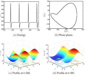
0.7≤ν1≤1are given in the first line of the table (lower values ofν1appearing in the second line of the Table are discussed below). The results indicate that the period decreases monotonically, albeit rather slowly, from a value of approximately 126.75at ν1= 1 to89.9at ν1= 0.7. This indicates that the persistence of the steady state attractor becomes weaker as ν1 decreases. An example of these homoclinic burst solutions is given in Figure 10 for (ν1, ν2) = (0.8,0.2). The energy E(t) and its corresponding phase plane (E,E˙), are shown in panels (a) and (b), respectively - the phase plane is a closed curve that is traversed a single time as the solution evolves over one period in time. The fast bursting dynamics connecting homoclinic states are clearly visible in these numerical results; the solution spends most of its time in the constant energy region and this corresponds to the corner-like part of the phase plane in the vicinity of

˙

(15)

15

rspa.ro

y

alsocietypub

lishing.org

Proc

R

Soc

A

0000000

..

100 200 300 400 500

200 250 300 350 400 450 500 550

t

E

(t

)

200 300 400 500 600

−150 −100 −50 0 50 100 150

E(t)

˙ E(t

)

(a)Energy. (b)Phase plane.

0 2

4 6

0 2 4 6 −5

0 5 10

y x

v

(

x

,

y

)

0 2

4 6

0 2 4 6 −5

0 5 10

y x

v

(

x

,

y

)

[image:15.595.155.446.112.368.2]

(c)Profile at t=360. (d)Profile at t=381.

Figure 10.Periodic homoclinic burst solutions forν1= 0.8andν1= 0.2. Panel (a) evolution of the energyE(t); panel

(b) phase plane of the energy; panel (c) solution att= 360on the constant energy plateau, and panel (d) solution at

t= 381taken during a burst.

ν1 1.00 0.95 0.90 0.85 0.80 0.75 0.70 Per 126.75 119 113.5 108.75 102.3 96.15 89.9

ν1 0.65 0.60 0.55 0.50 0.45 Per 2.79 2.66 2.57 2.54 2.68

Table 2.Oscillation period for time–periodic solutions with ν2= 0.2. For 0.7≤ν1≤1 the solutions are periodic

homoclinic bursts while for0.45≤ν1≤0.65, regular oscillations in the energy signal are observed.

state and an energy peak, at timest= 360andt= 381, respectively. For these values ofν1andν2, the steady solutions between bursts are unimodal inxand bimodal iny, that is the only non-zero Fourier modes aren1∈Zandn2= 2m2, m2∈Z.

Next we consider even lower values of ν1, that is we fix ν2= 0.2 and study the interval

(16)

16

rspa.ro

y

alsocietypub

lishing.org

Proc

R

Soc

A

0000000

..

two consecutive periods, respectively, att= 141.54andt= 144.08, are shown in panels (c)–(e). Interestingly, even though the energy completes one period of oscillation between each profile, we see that the solution requires two complete periods to return to its initial spatial form. This can be understood from the results in panels (c)–(e). Modulo a constant translation along the line

x=y, the solution in panel (d) is identical to those in panels (c) and (e). This can be seen from the projected contour plots of the solution onto thex−yplane; in panel (c) there is a “figure 8" feature (i.e. a saddle point for the surface) in the middle of the domain, and a rectangular feature (i.e. a local maximum for the surface) in the vicinity of the origin. After one period of oscillation has elapsed the solution is that shown in panel (d), and inspection of the projected contour plot confirms that the saddle and local maximum regions mentioned above are interchanged. This holds for any three solutions separated by one period of oscillation between them - we arbitrarily tookt= 139as the first solution in these results - and so the attractor is of traveling periodic type with the solution returning to its initial form modulo a spatial shift, after each period. We find all the solutions on the lineν2= 0.2have this distinctive feature.

(e) Quasi–periodicity and chaos

Next we decreaseν2further to the fixed valueν2= 0.15and varyν1in the interval0.35≤ν1≤

1; we find solutions supporting chaotic heteroclinic bursts along with quasi periodic and fully chaotic solutions - see Figure5. An example of a chaotic heteroclinic burst solution for(ν1, ν2) =

(0.85,0.15)is shown in Figure12; the energy evolution given in Figure12(a) switches between two different fixed points with energy approximately equal to 340and 300, respectively, and exhibits chaotic bursts in between - this is in contrast to the homoclinic bursts found at largerν2 -Figure10. Evidence of the chaotic nature of the bursts is found in the corresponding energy phase plane panel (b), which is composed of non-repeating trajectories. Panels12(c)–(e) present solution profiles att= 1100,1230,1300corresponding to times on the higher energy steady state attractor,

100 110 120 130 140 150

350 400 450 500 550

t

E

(t

)

350 400 450 500 550

−200 −100 0 100 200 300

E(t)

˙ E(t

)

0 2

4 6

0 2 4 6 −8 −4 0 4 8

y x

v

(

x

,

y

)

0 2

4 6

0 2 4 6 −8 −4 0 4 8

y x

v

(

x

,

y

)

0 2

4 6

0 2 4 6 −8 −4 0 4 8

y x

v

(

x

,

y

)

[image:16.595.118.482.442.695.2]

(c)Profile at t=139. (d)Profile at t=141.54. (e)Profile at t=144.08.

Figure 11.(a) Energy, (b) phase plane, and solution profiles for the periodic homoclinic solution at(ν1, ν2) = (0.5,0.2).

Panel (c) shows the solution profile at the minimum energy att= 139. Panel (d) shows the solution one period later (t =

(17)

17

rspa.ro

y

alsocietypub

lishing.org

Proc

R

Soc

A

0000000

..

1000 1500 2000 2500 3000

300 400 500 600 700 800

t

E

(t

)

300 400 500 600 700 800 −300

−200 −100 0 100 200 300

E(t)

˙ E(t

)

0 2

4 6

0 2 4 6 −5 0 5 10

y x

v

(

x

,

y

)

0 2

4 6

0 2 4 6 −10

−5 0 5 10

y x

v

(

x

,

y

)

0 2

4 6

0 2 4 6 −5

0 5 10

y x

v

(

x

,

y

)

[image:17.595.116.482.110.369.2]

(c)Profile at t=1100. (d)Profile at t=1230. (e)Profile at t=1300.

Figure 12.(a) Energy, (b) phase plane, and solution profiles for the periodic homoclinic solution at (ν1, ν2) =

(0.85,0.15). The profiles correspond to the solution at the (c) higher energy plateau, during the (d) chaotic burst and at the (e) lower energy plateau.

during the chaotic burst, and at the lower energy steady state, respectively. For the lower energy level (t= 1300, panel (e)), we find that the profiles are bimodal iny(i.e.y−periodic of periodπ), but unimodal during the upper energy level (e.g.t= 1100, panel (c)); during the chaotic bursts the solutions are also unimodal. We emphasise that for this particular example, only12Fourier modes are required in thex−direction, and30in they−direction to achieve double machine precision. We conclude then, that analogously to the 1D KSE [22], complex chaotic solutions exhibit low modal behaviour and can be well characterised by low order dynamical systems.

Asν1,ν2decrease further, complex behaviour persists and includes quasi–periodic oscillations in time (analogous to quasi–periodic flows on a torus with return maps - see Section5- consisting of densely filled curves as in Figure7(a)). Further decrease ofν1, ν2produces large time solutions that are mainly chaotic. This chaotic attractor does not emerge through homoclinic or heteroclinic bursting and assumes a more complicated structure as seen in the return maps of Figure7(b), for example, which exhibit no discernible patterns. Despite this, these solutions can be characterised by their statistical properties which we have done in Section3.

6. Conclusions

We presented an extensive numerical study of the 2D KSE equation (1.4), inspired by recent analytical studies [34,35] and encouraged by the success of understanding solution dynamics of the 1D KSE though careful and comprehensive numerical studies. The equation was solved on doubly periodic domains[2Lx,2Ly]with particular interest on large domain dynamics. For

L≫1we considered three cases: (i)Lx=Ly=L; (ii)Lx= 10,Ly= 10L; and (iii)Ly fixed and

(18)

18

rspa.ro

y

alsocietypub

lishing.org

Proc

R

Soc

A

0000000

..

L2in 2D), analogously to the 1D KSE [29]. We linked the long-wave energy spectrum to the form of the non-linearity in the 2D KSE, showing that it is responsible for both its radial symmetry in Fourier space and its ∼k−2_{dependence - see Figures} ₂_and₃_{. Extensive dynamics and the} equipartition of energy are recovered by differentiating the solution and considering the energy spectrum ofU1=vxandU2=vy. This is consistent with efforts [51,52] to model the large scale chaotic dynamics of the 2D KSE by the Kardar-Parisi-Zhang equation.

We also examined the solutions arising when bothν1=π2/L2x<1andν2=π2/L2y<1so that unstable modes are present and the solutions are fully two-dimensional. The ν1−ν2 solution phase space was mapped by solving a large number of initial value problems - see Figure5. For values close to the bifurcation point ν1=ν2= 1, we constructed asymptotic solutions that are in good agreement with the computations. Asν1, ν2decrease these bifurcated solutions become more nonlinear and unimodal fully 2D steady states emerge. For smaller (but still moderate) values ofν1,ν2, travelling waves and time–periodic solutions emerge, the latter appearing in the form of periodic homoclinic or heteroclinic bursts, or solutions with shapes that rapidly oscillate in time - these are similar to those found for the 1D KSE [23]. Solutions evolve to more complicated structures of quasi–periodic or chaotic nature asν1,ν2decrease sufficiently (equivalently as the domain size increases). These chaotic solutions can arise through an infinite number of paths in(ν1, ν2)-space, and we explored in detail the paths alongν1=ν2=ν→0, andν1 fixed with ν2→0. We found that the transition to chaos is via quasi–periodicity and did not observe the pattern of Feigenbaum period–doubling bifurcations found for the 1D KSE - [30].

Our computations suggest that the energy bounds of [34,35] in high aspect ratio domains could be extended to more general domain sizes and we suggest an optimalL2−bound proportional to the system size (equal toL2in our notation). While many of our results show that the 2D KSE and its solutions share features with the 1D KSE, we have also seen differences due to the additional dimension. Perhaps the most notable pertains to transitions to chaos. We have only explored in detail two of the infinitely many paths inν1−ν2space, and a closer examination of this aspect of the problem would be interesting. It would also be interesting to explore the effect of dispersion on the 2D KSE by including a term proportional to∆uxin (1.4). In 1D dispersion can regularise chaotic dynamics into travelling wave pulses [43]. In 2D there is limited work on equations similar to the differentiated form of the 2D KSE [42,53]; dispersion is found to transform chaotic solutions into travelling wave pulses, but in many cases these travelling waves are unstable in the sense that they do not emerge as solutions to initial value problems. This feature of the 2D problem is quite distinct that in 1D where moderate amounts of dispersion produce stable travelling wave pulses. It would be of interest to classify such effects for the 2D KSE.

Acknowledgment

The work of D.T.P. was partly supported by EPSRC grant EP/K041134/1; A.K. acknowledges a Roth Doctoral Fellowship from the Department of Mathematics, Imperial College London.

Data Accessibility

All data were computed by the authors using their own codes. These can be found at https://github.com/kalogirou/2D-Kuramoto-Sivashinsky .

Competing Interests

There are no competing interests.

Authors contribution statement

(19)

19

rspa.ro

y

alsocietypub

lishing.org

Proc

R

Soc

A

0000000

..

analysis of the study and interpretation of data, and edited the manuscript. All authors discussed the results and implications and commented on the manuscript at all stages. All authors gave final approval for publication.

References

1. Homsy, G. M. 1974 Model equations for wavy viscous film flow. In: Newell, A. C. (ed.)Nonlinear Wave Motion. Lectures in Applied Mathematics, 15, pp. 191–194. American Mathematical Society, Providence.

2. Nepomnyashchii, A. A. 1974 Stability of wavy conditions in a film flowing down an inclined plane.Translated from Izv. Akad. Nauk SSSR, Mekh. Zhidk. Gaza, 3, 28–34.

3. LaQuey, R. E., Mahajan, S. M., Rutherford, P. H.&Tang, W. M. 1975 Nonlinear saturation of the trapped-ion mode.Phys. Rev. Lett., 34, 391–394.

4. Kuramoto, Y. 1975 Diffusion–induced chaos in reactions systems.Progr. Theoret. Phys. Suppl., 54, 687–699.

5. Michelson, D. M.&Sivashinsky, G. I. 1977 Nonlinear analysis of hydrodynamic instability in laminar flames–II. Numerical experiments.Acta Astronautica, 4, 1207–1221, doi: 10.1016/0094-5765(77)90097-2.

6. Sivashinsky, G. I. 1977 Nonlinear analysis of hydrodynamic instability in laminar flames–I. Derivation of basic equations.Acta Astronautica, 4, 1177–1206.

7. Sivashinsky, G. I. 1980 On flame propagation under conditions of stoichiometry.SIAM J. Appl. Math., 39 (1), 67–82, doi: 10.1137/0139007.

8. Papageorgiou, D. T., Maldarelli, C.&Rumschitzki, D. S. 1990 Nonlinear interfacial stability of core–annular film flows.Phys. Fluids A, 2 (3), 340–352, doi: 10.1063/1.857784.

9. Tilley, B. S., Petropoulos, P. G.&Papageorgiou, D. T. 2001 Dynamics and rupture of planar electrified liquid sheets.Phys. Fluids, 13 (12), 3547–3563, doi: 10.1063/1.1416193.

10. Hooper, A. P.&Grimshaw, R. 1985 Nonlinear instability at the interface between two viscous fluids.Phys. Fluids, 28, 37–45, doi: 10.1063/1.865160.

11. Sivashinsky, G. I.&Michelson, D. M. 1980 On irregular wavy flow on liquid film down a vertical plane.Prog. Theor. Phys., 63 (6), 2112–2114, doi: 10.1143/PTP.63.2112.

12. Cohen, B. I., Krommes, J. A., Tang, W. M.&Rosenbluth, M. N. 1976 Non–linear saturation of the dissipative trapped ion mode by mode coupling.Nucl. Fusion, 16 (6), 971–992, doi: 10.1088/0029-5515/16/6/009.

13. Kuramoto, Y. & Tsuzuki, T. 1976 Persistent propagation of concentration waves in dissipative media far from thermal equilibrium. Prog. Theoret. Phys., 55 (2), 356–369, doi: 10.1143/PTP.55.356.

14. Cuerno, R&Barabáci, A.-L. 1995 Dynamic scaling of ion–sputtered surfaces.Phys. Rev. Lett., 74 (23), 4746–4749, doi: 10.1103/PhysRevLett.74.4746.

15. Collet, P., Eckmann, J.-P., Epstein, H. & Stubbe, J. 1993 A global attracting set for the Kuramoto–Sivashinsky equation.Comm. Math. Phys., 152, 203–214, doi: 10.1007/BF02097064. 16. Collet, P., Eckmann, J.-P., Epstein, H. & Stubbe, J. 1993 Analyticity for the Kuramoto–

Sivashinsky equation.Physica D, 67, 321–326, doi: 10.1016/0167-2789(93)90168-Z.

17. Goodman, J. 1994 Stability of the Kuramoto–Sivashinsky and related systems.Comm. Pure Appl. Math., 47 (3), 293–306, doi: 10.1002/cpa.3160470304.

18. Nicolaenko, B., Scheurer, B. &Temam, R. 1985 Some global dynamical properties of the Kuramoto–Sivashinsky equations: Nonlinear stability and attractors.Physica D, 16 (2), 155– 183, doi: 10.1016/0167-2789(85)90056-9.

19. Tadmor, E. 1986 The well–posedness of the Kuramoto–Sivashinsky equation.SlAM J. Math. Anal., 17 (4), 884–893, doi: 10.1137/0517063.

20. Frisch, U., She, Z.–S. &Thual, O. 1986 Viscoelastic behaviour of cellular solutions to the Kuramoto–Sivashinsky model.J. Fluid Mech., 168, 221–240, doi: 10.1017/S0022112086000356. 21. Hyman, J. M., Nicolaenko, B. &Zaleski, S. 1986 Order and complexity in the Kuramoto–

Sivashinsky model of weakly turbulent interfaces.Physica D, 23, 265–292, doi: 10.1016/0167-2789(86)90136-3.

22. Papageorgiou, D. T.&Smyrlis, Y.-S. 1991 The Route to Chaos for the Kuramoto–Sivashinsky Equation.Theor. Comput. Fluid Dyn., 3, 15–42, doi: 10.1007/BF00271514.

(20)

20

rspa.ro

y

alsocietypub

lishing.org

Proc

R

Soc

A

0000000

..

24. Il‘yashenko, J. S. 1992 Global analysis of the phase portrait for the Kuramoto–Sivashinsky equation.J. Dyn. Differ. Equ., 4 (4), 585–615, doi: 10.1007/BF01048261.

25. Jolly, M. S., Rosa, R. & Temam, R. 2000 Evaluating the dimension of an inertial manifold for the Kuramoto–Sivashinsky equation. Adv. Differ. Equ., 5, 31–66, doi: projecteuclid.org/euclid.ade/1356651378.

26. Bronski, J. R.&Gambill, T. N. 2006 Uncertainty estimates andL2bounds for the Kuramoto– Sivashinsky equation.Nonlinearity, 19, 2023–2039, doi: 10.1088/0951-7715/19/9/002. 27. Giacomelli, L.&Otto, F. 2005 New bounds for the Kuramoto–Sivashinsky equation.Comm.

Pure Appl. Math., 58 (3), 297–318, doi: 10.1002/cpa.20031.

28. Otto, F. 2009 Optimal bounds on the Kuramoto–Sivashinsky equation. J. Funct. Anal.257, 2188–2245, doi: 10.1016/j.jfa.2009.01.034.

29. Wittenberg, R. W.&Holmes, P. 1999 Scale and space localization in the Kuramoto–Sivashinsky equation.Chaos, 9 (2), 452–465, doi: 10.1063/1.166419.

30. Smyrlis, Y.-S.&Papageorgiou, D. T. 1991 Predicting chaos for infinite dimensional dynamical systems: The Kuramoto–Sivashinsky equation, a case study.Proc. Nati. Acad. Sci. USA, 88, 11129–11132.

31. Kukavica, I. 1994 Oscillations of solutions of the Kuramoto–Sivashinsky equation.Physica D, 76 (4), 369–374, doi: 10.1016/0167-2789(94)90045-0.

32. Gruji´c, Z. 2000 Spatial analyticity on the global attractor for the Kuramoto–Sivashinsky equation.J. Dyn. Differ. Equ., 12 (1), 217–228, doi: 10.1023/A:1009002920348.

33. Cao, Y.&Titi, E. S. 2006 Trivial stationary solutions to the Kuramoto–Sivashinsky and certain nonlinear elliptic equations.J. Differ. Equations, 231, 755–767, doi: 10.1016/j.jde.2006.08.002. 34. Sell, G. R.&Taboada, M. 1992 Local dissipativity and attractors for the Kuramoto–Sivashinsky

equation in thin 2D domains.Nonlin. Anal., 18, 671–687, doi: 10.1016/0362-546X(92)90006-Z. 35. Molinet, L. 2000 Local Dissativity inL2for the Kuramoto–Sivashinsky Equation in Spatial

Dimension 2.J. Dyn. and Diff. Eqns., 12 (3), 533–556.

36. Demirkaya, A. & Stanislavova, M. 2010 Long time behavior for radially symmetric solutions of the Kuramoto–Sivashinsky equation.Dyn. Partial Differ. Equ., 7 (2), 161–173, doi: 10.4310/DPDE.2010.v7.n2.a2.

37. Michelson, D. 2008 Radial asymptotically periodic solutions of the Kuramoto–Sivashinsky equation.Physica D, 237, 351–358, doi: 10.1016/j.physd.2007.09.009.

38. Demirkaya, A. 2009 The existence of a global attractor for a Kuramoto–Sivashinsky type equation in 2D.Discrete Contin. Dyn. Syst.Dynamical Systems, Differential Equations and Applications, 7th AIMS Conference, suppl., 198–207.

39. Rost, M.&Krug, J. 1995 Anisotropic Kuramoto–Sivashinsky equation for surface growth and erosion.Phys. Rev. Lett., 75 (21), 3894–3897, doi: 10.1103/PhysRevLett.75.3894.

40. Gomez, H. & París, J. 2011 Numerical simulation of asymptotic states of the damped Kuramoto-Sivashinsky equation.Phys. Rev. E, 83, 046702, doi: 10.1103/PhysRevE.83.046702. 41. Paniconi, M. & Elder, K. R. 1997 Stationary, dynamical, and chaotic states of the

two-dimensional damped Kuramoto-Sivashinsky equation.Phys. Rev. E, 56 (3), 2713–2721, doi: 10.1103/PhysRevE.56.2713.

42. Akrivis, G., Kalogirou, A., Papageorgiou, D. T. and Smyrlis, Y.-S. 2015 Linearly implicit schemes for multi-dimensional Kuramoto- Sivashinsky type equations arising in falling film flows.IMA J. Numer. Anal., in press.

43. Akrivis, G., Papageorgiou, D. T. and Smyrlis, Y.-S. 2012 Computational study of the dispersively modified Kuramoto-Sivashinsky equation.SIAM J. Sci. Comput., 34 (2), A792– A813, doi: 10.1137/100816791.

44. Pomeau, Y., Pumir, A.&Pelce, P. 1984 Intrinsic Stochasticity with Many Degrees of Freedom. J. Stat. Phys., 37 (1/2), 39–49, doi: 10.1007/BF01012904.

45. Toh, S. 1987 Statistical model with localised structures describing the spatio–temporal chaos of Kuramoto–Sivashisky equation.J. Phys. Soc. Jpn, 56 (3), 949–962, doi: 10.1143/JPSJ.56.949. 46. Yamada, T.&Kuramoto, Y. 1976 A Reduced Model Showing Chemical Turbulence.Prog. Theor.

Phys., 56, 681–683, doi: 10.1143/PTP.56.681.

47. Indireshkumar, K. & Frenkel, A. L. 1997 Mutually penetrating motion of self–organized two–dimensional patterns of soliton like structures.Physical Rev. E, 55 (1), 1174–1177, doi: 10.1103/PhysRevE.55.1174.

(21)

21

rspa.ro

y

alsocietypub

lishing.org

Proc

R

Soc

A

0000000

..

49. Pinto, F.C. 1999 Nonlinear stability and dynamical properties for a Kuramoto-Sivashinsky equation in space dimension two.Discrete and Continuous Dynamical Systems, 5 (1), 117–136. 50. Bergé, P., Pomeau, Y.&Vidal, C. 1984Order Within Chaos – Towards a Deterministic Approach to

Turbulence. Wiley–Interscience.

51. Boghosian, B. M., Carson, C. C. & Hwa, T. 1999 Hydrodynamics of the Kuramoto-Sivashinsky equation in two dimensions. Phys. Rev. Lett., 83 (25), 5262–5265, doi: 10.1103/PhysRevLett.83.5262.

52. Jayaprakash, C., Hayot F. & Pandit R. 1993 Universal Properties of the Two-Dimensional Kuramoto-Sivashinsky Equation. Phys. Rev. Lett., 71 (1), 12–15, doi: 10.1103/PhysRevLett.71.12.