Efficient Numerical Schemes for Computing Cardiac Electrical Activation over Realistic Purkinje Networks: Method and Verification

This is a repository copy of

Efficient Numerical Schemes for Computing Cardiac Electrical

Activation over Realistic Purkinje Networks: Method and Verification

.

White Rose Research Online URL for this paper:

http://eprints.whiterose.ac.uk/85316/

Version: Accepted Version

Proceedings Paper:

Lange, M., Palamara, S., Lassila, T. et al. (3 more authors) (2015) Efficient Numerical

Schemes for Computing Cardiac Electrical Activation over Realistic Purkinje Networks:

Method and Verification. In: Functional Imaging and Modeling of the Heart. 8th

International Conference, FIMH 2015, June 25-27, 2015, Maastricht, The Netherlands.

Lecture Notes in Computer Science, 9126 . Springer International Publishing . ISBN

978-3-319-20308-9

https://doi.org/10.1007/978-3-319-20309-6_49

[email protected] https://eprints.whiterose.ac.uk/

Reuse

Unless indicated otherwise, fulltext items are protected by copyright with all rights reserved. The copyright exception in section 29 of the Copyright, Designs and Patents Act 1988 allows the making of a single copy solely for the purpose of non-commercial research or private study within the limits of fair dealing. The publisher or other rights-holder may allow further reproduction and re-use of this version - refer to the White Rose Research Online record for this item. Where records identify the publisher as the copyright holder, users can verify any specific terms of use on the publisher’s website.

Takedown

If you consider content in White Rose Research Online to be in breach of UK law, please notify us by

Efficient Numerical Schemes for Computing

Cardiac Electrical Activation over Realistic

Purkinje Networks: Method and Verification

Matthias Lange1_{, Simone Palamara}2_{, Toni Lassila}1_,

Christian Vergara2_{, Alfio Quarteroni}3_{, and Alejandro F. Frangi}1

1

CISTIB, Department of Electronic and Electrical Engineering, The University of Sheffield, United Kingdom

{m.lange,t.lassila,a.frangi}@sheffield.ac.uk

2

MOX, Dipartimento di Matematica, Politecnico di Milano, Italy

{simone.palamara,christian.vergara}@polimi.it

3

Chair of Modelling and Scientific Computing, ´

Ecole Polytechnique F´ed´erale de Lausanne, Switzerland

[email protected]

Abstract. We present a numerical solver for the fast conduction system in the heart using both a CPU and a hybrid CPU/GPU implementation. To verify both implementations, we construct analytical solutions and show that theL2

-error is similar in both implementations and decreases linearly with the spatial step size. Finally, we test the performance of the implementations with networks of varying complexity, where the hybrid implementation is, on average, 5.8 times faster.

1

Introduction

The cardiac Purkinje fibre network is an important contributor to the coordi-nated contraction of the heart as it can provide a fast conduction system reaching out to large areas of the sub-endocardium. The Purkinje fibres form an exten-sively branching and rejoining network, which is important for the reliability and fault-tolerance of the propagation of the action potential [1][2]. The ability to simulate propagation in physiological Purkinje networks is essential for stud-ies of the healthy heart to obtain realistic activation patterns [3, 4].It is equally important in the simulation of pathological hearts, where disturbances in the conduction system can alter the activation pattern greatly, e.g. bundle branch blocks and long duration ventricular tachycardia [5].

Typically the simulation of the action potential propagation in a Purkinje network is based on the bidomain equations [6], or on the cable equation with a reaction term [7]. The approach of Vigmondet al._{[7] treats the Purkinje}

con-duction system as a branching tree of conducting segments without loops. Our approach also allows current loops in the Purkinje network, which are observed in realistic Purkinje networks [2].

We present first briefly the approach of Vigmondet al._{, and then explain its}

present a simple model with exact known solution and use it for verification of both solvers. Finally, we compare the performance of both implementations.

2

Methods

2.1 Mathematical Model and Solution Method

The electrophysiology of cardiac tissue can be described either by the bidomain or the monodomain model. The former assumes an extracellular and intracellular space with different anisotropic conductivity tensors; if these tensors are linearly dependent the model reduces to the monodomain model [7].

The monodomain equation is considered in one dimension, because the Purk-inje network can be approximated by a network of 1-D line segments. Here we assume that the extracellular space is not affected by the Purkinje network, and ignore it in the following. The monodomain equation reads

∂x(σi∂xVm) =β(Cm∂tVm+Iion(Vm, ξ)), (1)

where xis the local coordinate,Vm is the transmembrane potential,Iion is the

current that flows through the ion channels, ξ are the state variables of the membrane model, β is the surface-to-volume ratio of the cell membrane, where σi is the intracellular conductivity, andCm is the membrane capacitance.

To derive a coupling condition between two or more line segments, needed to complete (1), we follow the idea of Vigmondet al._{[7]. The equations on each}

line segment are coupled together by a boundary condition resulting from the enforcement of continuity of the potential and the conservation of charges (Kirch-hoff’s law). To satisfy the boundary conditions, the transmembrane potential, VM, and the current,I, are needed. SinceI=σ∂xVm, the spatial derivatives of

the potential need to be computed. The system is discretized using a cubic Her-mite finite element method (FEM), which allows the currentI to be recovered as a continuous quantity.

In view of the numerical discretization with the Finite Element Method, each node of the mesh is assumed to be located in the gap junction between two cells, where the unknowns are the intracellular potentialφi and the current

Ig through the gap junction. Two ghost nodes are created on both sides of the

gap junction, where the transmembrane potentialV±, and ionic channel current Iionare defined. The advantage of the ghost nodes is that with the gap junction

modelled as a resistorR, the currentIg can be obtained from Ohm’s law

V±=φi−φe∓

IgR

2 , (2)

whereφe is the extracellular potential, taken constant in this work.

To correct for the introduced gap junction resistance, we use the equivalent conductivity σ∗

andρthe radius. This means, thatσiis the conductivity in the cell only, whileσ∗

is the conductivity of the cell and the gap junction. In this notation (1) becomes

∂x(σ∗∂xφ±i ) =β(Cm∂tV±+Iion(V±, ξ±)) , (3)

whereφ±i is the intracellular potential in the ghost nodes. Furthermore, we apply

an operator splitting technique to (3):

∂tV +L1(V) = 0

∂tV +L2(V) = 0 , (4)

where L1 =Iion is part of the differential operator that represents the

nonlin-ear term of (3), whereasL2 =∂x(σ∗∂x) represent the diffusion term of (3). A

fractional-step method with a discretization of the temporal derivatives by a first-order approximation is introduced, where the superscript n refers to the numerical solution computed at timetn_:

Vn+1/2_−Vn

∆t =−L1(V

n_), Vn+1−Vn+1/2

∆t =−L2(V

n+1_{). (5)}

Algorithm 1to Solve the Cable Equation with a Splitting Scheme

Step 1.Recover the transmembrane potentialV±nwith (2) fromIgn,φni,φne. Step 2.Solve the first equation of the (5), which is the update of the ionic current in the ghost nodes

V±n+1/2=V

n

±−

I_ion(V±n, ξ)

Cm

∆t . (6)

Step 3. ComputeφiandIg with the new values ofVn

+1/2

± in the real node:

φn_i+1/2= V

n+1/2 + +V

n+1/2

−

2 +φ

n e , In

+1/2

g =

V+n+1/2−V

n+1/2

−

R . (7)

Step 4. Use the FEM for the second stage of the operator splitting. By noticing

φi=φ

+ i+φ−i

2 and using the linearity ofL2, we find:

βCm∂t(φi−φe) =∂x(σ

∗

∂xφi) . (8)

Introducing a discretization in time results in:

βCm

(φn+1

i −φn

+1

e )−(φ n+1/2

i −φne)

∆t =∂xσ

∗

∂xφn

+1

i , (9)

which is solved with the FEM with 1-D cubic Hermite shape functions.

line segments. In the case that segment 1 bifurcates into segments 2 and 3, we enforce the continuity of the potential φ1 = φ2 =φ3 and the conservation of

current I1 =I2+I3. In contrast to Vigmondet al., our implementation covers

the case where segments 1 and 2 join to from segment 3, in which case the coupling condition of the currents is I1 = I3−I2. These boundary conditions

are introduced in the FEM system matrix associated to (9) and the right hand side.

2.2 Hardware Implementation

We now outline the CPU and the CPU/GPU hybrid implementations. The solver for the cable equation used the FEM in Step 4, and was implemented using the LifeV_{library (http://www.lifev.org) . Parallelism was achieved using OpenMPI.}

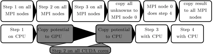
We parallelized only Steps 1-3 of the algorithm and solve the linear system in Step 4 serially. The reason for this is that calculating the ionic model can be done without knowing the mesh geometry and is computationally intensive. On the other hand, it is less trivial to parallelize the solving of the linear system. The resulting computational workflow is shown in Fig. 1.

The Steps 1, 3, and 4 were always implemented on the CPU, only Step 2 is run on the GPU. In the hybrid implementation, between Steps 1 and 2, an additional copy of the transmembrane potentialV±from the CPU to the GPU is made. To minimize the time spent copying the data, CUDA streams are used, which allow asynchronous tasks to be queued to the CPU. All computations were performed with Dell a Precision-WorkStation-T7500 featuring two Intel(R) Xeon(R) CPUs E5620 at 2.40GHz and NVIDIA Quadro 4000 GPU with 256 CUDA Cores.

Step1onall

MPInodes

Step2onall

MPInodes

Step3onall

MPInodes

opyall

unknownsto

MPInode0

MPInode0

doesstep4

opyresult

toallMPI

nodes

Step1

onCPU

Copypotential

toGPU

Step2onallCUDAores

Copypotential

toCPU

Step3

withCPU

Step4

withCPU

Fig. 1.Workflow for the CPU (above), and CPU/GPU hybrid (below) implementation. The CPU implementation needs to copy the potential in the gap junctions and the current, while the hybrid implementations needs to copy the potential of the ghost nodes. White boxes represent CPU tasks, and grey GPU tasks.

3

Numerical Experiments

estimate the absolute error and then to carry out a convergence test. The second experiment compares the performs of the CPU and CPU/GPU hybrid algorithm.

3.1 Numerical Error and Convergence

We first introduce a simplified model and develop two test problems with ana-lytical solutions. The non-physiological model is [8]

∂tV =pV, (10)

whereV is the transmembrane potential andpis a model parameter. Depending on the sign ofpthe cells are stable (p <0) and return exponentially to 0, or are unstable (p >0) and the transmembrane potential increases exponentially.

Next, we introduce two different test cases and derive their analytical solu-tions. For the first case the domainD1considered is an infinite line, which is

com-posed of three subintervalsD1,1= (−∞,−a),D1,2= [−a, a], andD1,3= (a,∞).

InD1,2 unstable cells are assumed, while in the surrounding regionsD1,1, D1,3

the cells are stable, with results in a spatial depend parameter of the simplified model

p(x) =

p2 forx∈D1,2

−p1 otherwise , (11)

wherep1, p2>0. Inserting the cell model in (1), we need to solve

Cm∂tV =δ∂x2V −p(x)V

V1(−a) =V2(−a) , V2(a) =V3(a)

V′

1(x)|x=−a= V

′

2(x)|x=−a , V

′

2(x)|x=a=V

′

3(x)|x=a

V1(−∞) = 0 , V3(∞) = 0,

, (12)

withδ=σ∗

/β. The solution presented by Artebrantet al._{[8] is}

V =

  

 

c1e

√

p1/δx _{x <}

−a cos(p

p2/δx)kxk ≤a

c1e−

√

p1/δx _{x > a}

with,p1=p2tan

2₍p

p2/δa),

c1= cos(−

p

p2/δa)e

√

p1/δa , (13)

whereaandp2 are the model parameters.

In the second test case, the domain D2 is a double-bifurcation with an

analytical solution. The domain consist of two rays, D2,1 = (−∞,−a) and

D2,2 = (−∞,−a) joining to form a line segment D2,3 = [−a, a] in the

mid-dle, which then splits again into two raysD2,4= (a,∞), D2,5= (a,∞), resulting

in a domain of five subintervals in total. The line segmentD2,3consists of active

cells, while all the rays consist of passive cells. The problem is symmetric with respect to zero, so we will look at the negative domain only. Furthermore, the raysD2,1 and D2,2 are identical, thus it suffices to solve the following problem

for only one of them:

δV′′

1 −p1V1= 0, ∀x∈D2,1

δV′′

3 +p2V3= 0, ∀x∈D2,3

V1(−a) =V3(−a), 2V1′(x)|−a =V3(x)

′

|−a, V1(−∞) = 0 ,

where the two in the derivatives is a result of Kirchhoff’s current law. The solution is very similar to the problem on one infinite line, with the ansatz functions V1 =c1ek1x,V3=c3cos(k2x) the constantc1 is still given by (13). A

relation betweenp1 andp2 follows from

2V′

1(−a) =V3′(−a) (13)

⇒ 2k1(c3cos(−k2a)ek1a)e−k1a=−k2c3sin(−k2a)

⇒p1=p2₄ tan2(

p

p2/δa).

(15)

Again, we need to fixV3 at one point to get a unique solution.

Timing CPU Hybrid 0 100 200 300 400 500 600 time in s Startup Diusion Reation CPU Hybrid 0 100 200 300 400 500 600 time in s CPU Hybrid 0 100 200 300 400 500 600 time in s CPU Hybrid 0 100 200 300 400 500 600 time in s Network

Nodes 6251 16 024 31 319 43 748

Table 1.The computational time for different Purkinje networks in the left ventricle (LV) and right ventricle (RV).

Comparison of the Absolute Error: For numerical simulations, we used the parameters p2 = 1 µF/ms, a = 1cm, Cm = 1µF, and c2 = 1. The cell

length has been chosen to l = 62.5 µm_{, and a radius of ρ= 16.0µ}m_{, which is}

within the physiological limits [9]. Furthermore, we make the arbitrary choice δ= 1 [kS/cm2_{], R= 0.1kΩ and recall, thatδ=σ}∗_{/β, from which we find the} conductivityσi= 1967 [kS/cm]. The spatial discretisation stephis then chosen

to be a integer multiple of l, i.e.h=nl, n ∈N_{, which means that each finite}

−10 0 10 0

5 ·10−2

x

Absolute

Error

−10 0 10

0 5 ·10−2

x

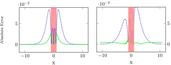
Fig. 2.The absolute error between the analytic solution of the potential and the numer-ical solution. For the test case on an infinite line (left), and for the simple branching network (right), where the dotted line has a step size of 0.1 cm, while the solid is 0.00625 cm and the error is multiplied by 10. The active cells are in the mark region.

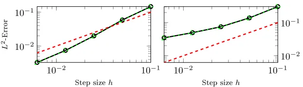
Convergence Test: For the error convergence test, we ran the simulation with the same parameters as before forn={1,2,3,4,5}in the spatial discretisation and calculated theL2_{-Error for each step size (Fig. 3). The CPU and CPU/GPU}

hybrid implementation give the same linear convergence of the error. We conjec-ture that the fourth order of convergence, which is expected for Hermit bases, is not reached because of the step 1 and 3.

3.2 Performance Comparison

4

Conclusion

10−₂

10−₁ 10−2

10−₁

Stepsizeh

L

2-Error

10−₂

10−₁ 10−2

10−₁

Stepsizeh

Fig. 3.Linear convergence inh(dashed line) and the convergence rates of the potential computed with the CPU (dotted line), and from the CPU/GPU hybrid (solid line). Results are for the single line case (left) and for the simple branching network (right).

We presented an extension of the work of Vigmondet al._{to solve more}

re-alistic Purkinje networks, and implemented it both on a CPU and in a hybrid CPU/GPU architecture. To evaluate the accuracy of both we performed a con-vergence test of theL2_{-Error, and showed that the solver converges linearly with}

the step size. The branching points introduce a small additional error in the nu-merical solution. Both implementations had equivalent nunu-merical accuracy.

The performance test indicated that the hybrid implementation using 256 CUDA cores and 1 CPU was in average 5.8 times faster than the CPU imple-mentation run with 8 CPUs. This motivates our future work on developing an implementation, which performs all the remaining steps of the algorithm on the GPU to realize even greater performance gains.

Acknowledgements

Simone Palamara has been funded by “Fondazione Cassa di Risparmio di Trento e Rovereto” (CARITRO) within the project “Numerical modelling of the electri-cal activity of the heart for the study of the ventricular dyssynchrony”. Christian Vergara has been partially supported by the Italian MIUR PRIN09 project no. 2009Y4RC3B 001.

References

[1] Cooper, L.L., Odening, K.E., Hwang, M.-S., Chaves, L., Schofield, L., Taylor, C., Gemignani, A.S., Mitchell, G.F., Forder, J.R., Choi, B.-R., Koren, G.: Electrome-chanical and structural alterations in the aging rabbit heart and aorta. Am. J. Physiol. Heart Circ. Physiol. 302, H1625–H1635 (2012)

[3] Vergara, C., Palamara, S., Catanzariti, D., Nobile, F., Faggiano, E., Pangrazzi, C. Maurizio Centonze, Massimiliano Maines, Alfio Quarteroni, Giuseppe Vergara : Patient-specific generation of the Purkinje network driven by clinical measurements of a normal propagation. Med Biol Eng Comput, 52(10), 813–826, (2014)

[4] Palamara S., Vergara C., Catanzariti D., Faggiano E., Centonze M., Pangrazzi C., Maines M., Quarteroni A.: Computational generation of the Purkinje network driven by clinical measurements: The case of pathological propagations. Int. J. Num. Meth. Biomed. Eng., 30(12), 1558–1577, (2014)

[5] Bogun, F., Good, E., Reich, S., Elmouchi, D., Igic, P., Tschopp, D., Dey S., Wim-mer, A., Jongnarangsin, K., Oral, H., Chugh, A., Pelosi, F., Morady, F.: Role of Purkinje Fibers in Post-Infarction Ventricular Tachycardia. J Am Coll Cardiol. 48(12), 2500–2507 (2006)

[6] Bordas, R.M., Gillow, K., Gavaghan, D., Rodriguez, B., Kay, D.: A Bidomain model of the ventricular specialized conduction system of the heart. SIAM J. Appl. Math. 72, 1618–1643 (2012)

[7] Vigmond, E.J., Clements, C: Construction of a computer model to investigate saw-tooth effects in the Purkinje system. IEEE Trans. Biomed. Eng. 54, 389–99 (2007) [8] Artebrant, R., Tveito, A., Lines, G.T.: A method for analyzing the stability of the resting state for a model of pacemaker cells surrounded by stable cells. Math. Biosci. Eng. 7, 505–526 (2010)

[9] Stankovicov´a T, Bito V, Heinzel F, Mubagwa K, Sipido KR.: Isolation and Mor-phology of Single Purkinje Cells from the Porcine Heart. Gen Physiol Biophys. 22(3), 329–340 (2003)

[10] Sebastian, R., Zimmerman, V., Romero, D., Frangi, A.F.: Construction of a com-putational anatomical model of the peripheral cardiac conduction system. IEEE Trans. Biomed. Eng. 58(12), 3479–3482 (2011)