Wireless body area network platform utilizing energy-efficient routing of physiological data

Rochester Institute of Technology

RIT Scholar Works

Theses

Thesis/Dissertation Collections

9-23-2011

Wireless body area network platform utilizing

energy-efficient routing of physiological data

Alvaro Prieto

Follow this and additional works at:

http://scholarworks.rit.edu/theses

This Thesis is brought to you for free and open access by the Thesis/Dissertation Collections at RIT Scholar Works. It has been accepted for inclusion in Theses by an authorized administrator of RIT Scholar Works. For more information, please [email protected].

Recommended Citation

Wireless Body Area Network Platform Utilizing

Energy-Efficient Routing of Physiological Data

by

Alvaro Prieto

Master of Science Thesis

in

Electrical Engineering

Approved by:

(Gill Tsouri, Ph. D.)

(Andres Kwasinski, Ph. D.)

(Nirmala Shenoy, Ph. D.)

(Sohail A. Dianat, Ph. D.)

Electrical and Microelectronic Engineering Department

Kate Gleason College of Engineering

Rochester Institute of Technology

Rochester, New York

[email protected]

Contents

Table of Contents 2

Abstract 4

List of Figures 5

1 Previous Work 7

1.1 Time Synchronization . . . 7

1.2 Synchronized Sampling . . . 10

1.3 Routing and Relaying . . . 10

2 Software Libraries 12 2.1 Project History . . . 12

2.2 Design Choices . . . 13

2.3 CC430 Device . . . 13

2.4 MSP430-RF2500 Device . . . 14

3 Wireless ECG Application 14 3.1 Description . . . 14

3.2 TinyOS Platform . . . 15

3.3 CC430 Platform . . . 15

3.4 Time Synchronization . . . 15

3.5 Scheduling . . . 16

3.6 Host Interface . . . 18

4 Algorithm Development Platform 18 4.1 Initial Development . . . 18

4.2 Hardware Coupling . . . 19

4.3 Simulation Output . . . 20

5.2 Proposed Cost Function . . . 23

5.2.1 Device Energy . . . 23

5.2.2 Link Cost . . . 23

5.2.3 Assumptions . . . 24

5.3 Performance Analysis . . . 24

5.3.1 Algorithm Implementation . . . 24

5.4 Simulation . . . 24

5.5 Hardware Implementation . . . 26

5.5.1 Hardware Platform . . . 26

5.5.2 Cycle of Operations . . . 26

5.5.3 Details . . . 27

5.6 Results . . . 29

Abstract

Wireless Body Area Networks (WBANs) consist of several wireless sensors located around a human

body. These sensors may measure several biological signals, movement, and temperature. Due to

major improvements in power consumption and constantly shrinking devices, WBANs are becoming

ubiquitous. As a side effect present because of the small form factor of these devices, the battery

size is limited. While the sensors themselves may be extremely power efficient, all of the measured

data must be transmitted over a much less efficient wireless link. One benefit of WBANs is that

they rarely include more than a dozen wireless devices over a small area. This constraint allows for

the use of routing techniques not suitable for larger wireless sensor networks(WSNs).

Presented in this work is a novel global routing algorithm link-cost function to maximize network

lifetime in WBANs. Also included are a basic software framework for developing WBANs, a

sam-ple Wireless Electrocardiogram (ECG) application, and a simsam-ple link cost algorithm development

List of Figures

1 RBS Multi-Hop Network Layout. From [6]. . . 8

2 EZ430-RF2500 with Battery Pack . . . 14

3 Test Network Layout . . . 16

4 Synchronization Test . . . 17

5 System Schedule . . . 18

6 Sample Measurement from Single ECG Lead . . . 19

7 Sample Network Visualization . . . 20

8 Sample Run-time Output . . . 21

9 Experimental Setup (Not all links shown) . . . 22

10 Walking environment. . . 27

11 Subject with devices for RSSI capture . . . 28

12 Sitting M=0 . . . 29

13 Sitting M=100 . . . 30

14 Walking M=0 . . . 31

15 Walking M=100 . . . 31

Summary of Contributions

The following is a list of contributions presented in this work.

• Software platform for WBAN research. - The software platform was developed using

only free and open source software (FOSS) tools. Radio libraries for the Texas Instruments

(TI) CC430 device were ported over from TI reference code, while libraries for the CC2500

radio were written from scratch. Other features include timer control for scheduling and

time-stamping, serial communication, some digital I/O, and analog input. Included in the platform

were limited software tools for data capture and visualization on a host computer.

• Wireless ECG platform- In order to test and demonstrate the WBAN platform, a wireless

ECG system was implemented. The system included three wireless devices, an access point,

and a host computer. Software for synchronized sampling was developed and tested successfully

using the WBAN platform. Three ECG leads were sampled at 300Hz and displayed on a host

computer in real-time.

• Software platform for routing algorithm development - In order to develop a novel

routing algorithm, a platform to test and compare with others was developed. The application

uses Dijkstra’s algorithm for best path selection, and allows for the testing of various link-cost

functions. Both simulation and real-time operation are supported. One unique feature is the

generation of routing graphic generation for network visualization.

• Specialized cost function for maximizing WBAN lifetime using global routing

al-gorithms- A novel routing algorithm is developed that focuses not on single devices, but the

network as a whole. Current methods focus on maximizing individual device lifetime or

min-imizing the energy-per-bit. While those are generally good goals, certain systems require all

devices functioning to be considered operational. Keeping that in mind, the proposed system

maximizes the network lifetime by normalizing power use across the network. For the purpose

of this paper, network lifetimeis defined as the time it takes any single node to deplete its

energy source.

• Publication A. Prieto, G. R. Tsouri, ”Efficient Global Routing Algorithm for Prolonging

Network Lifetime in Body Area Networks”, in preparation IEEE Wireless Communication

1

Previous Work

1.1

Time Synchronization

Time synchronization has been the subject of research for many years.

There are robust and time-tested synchronization methods, such as the Network Time Protocol

(NTP) [10], which are currently in use around the world. Unfortunately these methods were designed

for wired systems, and do not perform well once power consumption, latency, and other wireless

effects taken into account.

One of the first synchronization protocols designed specifically for wireless networks is Reference

Broadcast Synchronization (RBS) [6]. The main idea behind RBS is to synchronize all wireless

sensor nodes to each other. This creates a local time, within the network of nodes, where all clocks

are synchronized. For many applications, sensor nodes do not need to know the actual time, as

long as they are synchronized to one another. [6] lists an example application that measures the

time-of-flight of sound. If needed, RBS can be extended to use an external global time source to

provide a relate the local and global times.

There are several sources of nondeterminism in a wireless network. [6] and [9] decompose the

sources of nondeterminism into several components. These components account for the delays due

to the sending and receiving of a message in a wireless network. These components(from [6]) are:

• Send Time – Time the sender takes to construct a message. Includes delays incurred by the operating system and time required to transfer the message from the host to the network

interface.

• Access Time – Time spent waiting for access to transmit channel.

• Propagation Time – Time taken by the message to physically travel from sender to receiver. • Receive Time – Time spent processing a message and notifying the host of its arrival. As suggested by its name, RBS uses broadcast messages to synchronize wireless nodes to one

another. RBS does not synchronize a set of wireless nodes to a reference clock. Because of this

property, RBS effectively eliminates the Send Time and Access Time as sources of error. The

assumption if all nodes are equidistant from the broadcast message source. As stated in [14], the

main benefit of RBS was due to high transmission nondeterminism. With new radio technology, this

is no longer the main problem.

RBS is expandable for multi-hop networks, but has several requirements to do so. The first is

that there must be multiple broadcast transmitters in order to cover the whole network. This creates

several sub-networks of synchronized nodes, but does not synchronize them all together. The second

requirement is that there must be a sort of overlap between broadcast transmitters. A sensor node

receiving broadcasts from two different transmitters can compute the offset between the local times

of both networks.

Figure 1: RBS Multi-Hop Network Layout. From [6].

Another time synchronization protocol introduced in [7] is the Timing-sync Protocol for Sensor

Networks (TPSN). In contrast to RBS, TPSN synchronizes a set of notes to a single global time

source. A hierarchical structure is established before synchronization can take place. Once the

structure is in place, the root node begins to synchronize all nodes directly connected to it. Those

nodes then do the same for their children nodes, etc...

TPSN utilizes the sender-receiver approach [10] to synchronize a pair of nodes. A two-way

message exchange provides enough information to calculate the clock difference and propagation

delay between a pair of nodes. In order to synchronize the whole network, the root node initiates

the process. In order to reduce packet collisions, each child node waits for a random amount of time

are all synchronized. Due to the very structured nature of TPSN, special protocols are provided for

dealing with dying nodes, as well as newly introduced ones.

One of the costs of using TPSN over RBS is that theSend Time is once again a source of error in the system. This is, however, mitigated by closely integrating TPSN at the Medium Access Control

(MAC) layer. TPSN requires that both incoming and outgoing messages be timestamped at the

MAC level in order to minimize uncertainties in transmit and receive times.

The Flooding-Time Synchronization Protocol (FTSP) [9] is another protocol specifically designed

for resource limited wireless platforms. Like TPSN, FTSP relies on MAC-layer time-stamping, along

with several other new techniques, to synchronize devices. FTSP uses a single message to synchronize

the clocks of to wireless nodes. By comparison, RBS uses a single message to synchronize the clocks of

several devices to one-another, but not to the senders clock. TPSN uses two messages to synchronize

two device clocks. Because of this, FTSP needs to account to other sources of error, such as the

Byte Alignment Time. All three protocols are susceptible to the jitter inInterrupt Handling Time. In FTSP, each device sends a broadcast message with its clock time. Devices in the vicinity

listen to the broadcast and calculate the difference between their local and received times. In order

to reduce jitter, FTSP records multiple times to compute a singe, more accurate time-stamp. This

occurs on both the sending and receiving sides.

Another important contribution from FTSP is a method to deal with clock drift. Due to

dif-ferences in the exact frequency between local clocks, the time-difference between them grows over

time. [9] proposes a solution that takes place off-line. In the short-term, the clock drift is fairly

linear. Because of the linear fashion of clock drift, linear regression can be used to distribute the

error over a period of time. If clocks are being synchronized everyX seconds, and clocks drift some amountY, the algorithm distributes the driftY over all samples in aX second interval. The reason this must be done off-line is becauseY can only be computed after each synchronization.

FTSP scales well to multi-hop wireless networks. Reference points are utilized to keep track of

the time differences between the root node and the local node. FTSP is also resistant against losing

nodes as it includes root re-election protocols in case the root node fails. According to [14], FTSP

is currently thede factotime synchronization protocol in wireless sensor networks.

The Gradient Time Synchronization Protocol (GTSP) [16] focuses on synchronization of close-by

nodes in multi-hop networks. If two physically nearby nodes are part of two different synchronization

order to provide a more accurate time in relation to close-by nodes.

There are certain disadvantages to each of these methods. RBS requires additional messages

for time synchronization across multi-hop networks. TPSN does not account for the clock drift of

sensor nodes. Both RBS and TPSN are vulnerable to jitter in interrupt handling and decoding

times. While FTSP accounts for interrupt handling jitter, it does not take propagation time into

account. This is not a problem if nodes are physically close, but can affect performance in long

distance cases. GTSP and RBS are also vulnerable to propagation delay errors.

1.2

Synchronized Sampling

There are several applications, such as monitoring an active volcano [2], structural monitoring [18]

and counter sniper systems [15], which rely on synchronized measurements across sensor networks.

Currently there is not much research focusing specifically on synchronized sampling in low-power

WSNs. Apart from [17], most research utilizes the previously described time synchronization

protocols to keep device clocks aligned. With synchronized clocks, synchronized sampling is no

longer a complex problem.

1.3

Routing and Relaying

Due to power and physical constraints, sensor nodes placed along the body may not be able to

communicate with the main node directly. Even when sensor nodes are able reach the main node,

the power required to do so could be prohibitive. The use of relays to re-transmit the data has been

shown to dramatically reduce power consumption in body sensor networks [13].

There are several routing protocols currently used in WSNs [1], unfortunately, most are not well

suited for WBANs. Several of the protocols focus on mobility, Quality of Service (QoS), scalability

and reliability, among other things. In general, WBANs do not have the same requirements as other

WSNs. For example, in WBANs, scalability is no longer a problem since networks are limited to a

human body. In most cases, power consumption becomes the main limiting factor for overall system

performance.

Some routing protocols are specifically designed with WBAN constraints in mind. One example

is the Wireless Autonomous Spanning tree Protocol (WASP) [3]. Braem et al. describe the WASP

The main idea is that each node sends a “WASP-scheme” through a broadcast message that both

parent and children nodes receive. This scheme contains the time allotments for each node for the

current time frame. The children of the current node need the scheme to know when they are allowed

to transmit data. The scheme also informs the parent of the current node as to how many children

each node has, which allows it to allocate enough time slots for that branch. This method allows

for a distributed time-allocation protocol. Each time frame also includes contention periods where

new nodes can join the network. Routing is simple as data from sensor nodes is just sent up the

network tree and broadcast messages are used to send configuration down from the root node. The

main disadvantage of the WASP is the need to send the scheme packets from the root node down

the tree during every time frame.

An improvement over the WASP is the Cascading Information retrieval by Controlling Access

with Distributed slot Assignment (CICADA) protocol [8]. The improvement over the WASP has

to do with the separation of control and data subcycles. The WASP re-configures the time slots

during every frame, which produces a significant time delay. The information has to move from the

root node to all the children and back. The CICADA protocol configures the network in a separate

subcycle and later transfers data. The data transfer is initiated from the bottom of the tree, so there

is no delay waiting for the root node to send configurations down during each data subcycle.

Other WBAN routing methods focus on postural mobility [12]. Quwaider et al. propose a

protocol tolerant to constant network changes due to body/sensor movement. When sensor nodes

are located in body extremities, the wireless links vary with body position changes. The proposed

protocol uses a store-and-forward method to transfer data from sensor nodes to the main node.

While the protocol is well suited for dealing with mobile nodes, it requires more energy to do so.

“Hello” packets are constantly sent by each node to determine what the current neighboring nodes

are. A neighbor table is generated using this information and is necessary to determine where

packets will be sent to. Another problem with the method is due to multiple copies of packets being

transmitted to increase the probability of delivery. Finally, the main node transmits at full power

in order to poll each sensor node, increasing its energy consumption.

Most current routing methods for WBANs use network trees. One of the main problems present

with network trees is that the nodes closer to the main node deplete their energy supply faster than

children nodes. This is due to the fact that all trafic from children nodes has to be relayed through.

Using dedicated relays increases the individual sensor life, with the added cost of more devices.

So far, most WBANs have used tree-like networks to join nodes together. Tree networks, while

simple, are negatively affected by node failures and movement. Nabi et al. use a gossiping data

routing strategy along with TDMA based MAC to transmit information to the main node [11]. Each

node receives and stores the last sample data from every neighboring node. During transmission, it

sends its own sampled data, along with one or more of the stored packets from other nodes. This

method maximizes the likelihood of a packed reaching the main node, while consuming more power

due to retransmissions of the same data. Timestamps are used to decide whether or not a received

packed will be stored or discarded. The main node is assumed to have higher battery capacity and

transmission range. It is required to be able to reach all nodes with a single transmission. It is

in charge of sending a synchronization beacon to use as a time reference for TDMA frames. This

method is not always feasible, for example, when two nodes are on opposite sides of the body.

Another valuable contribution from [11] deals with Transmit Power Adaptation (TPA). The goal

for TPA is to minimize power consumption while maintaining a specific link quality. It achieves

this goal by adjusting Tx power according to link quality. Unlike the link quality metric in [12],

which was bidirectional, nodes have both inlink and outlink qualities. The outlink metric is then

maintained within predefined thresholds by varying Tx power. Inlink quality is stored and later

transmitted in order to share the information with neighboring nodes.

2

Software Libraries

One of the primary contributions of this project consists of software libraries for working with

WBANs. Due to the project requirements, a choice was made to use free and open source tools,

as opposed to proprietary software. Because of this choice, most of the radio libraries had to be

either ported or re-written from scratch. There were two main hardware devices that were targeted

in these libraries. The first consisted of a CC430 device, which has a built in 915MHz radio. The

second was an MSP430 with an external CC2500 2.4GHz radio.

2.1

Project History

The first software libraries were initially developed by Corey Provencher, a student at RIT, for a

movements and the corresponding software to use it. All of his software development was done using

the Texas Instruments (TI) software tools on Windows(TM).

Jeffery Robble, another student, took over and ported most of the code to use Linux based

open source tools. The code ported over by Robble used TI’s radio stack SimpliciTI. Unfortu-nately, SimpliciTI was too complex and resource heavy to do time-sensitive operations, like clock

synchronization, over the radio. It also required the use of other TI software libraries in order to

work.

After Robble left, the work continued. The main goal of the project at the time was to develop

wireless electrocardiogram(ECG)(Section 3). While planning for the wireless ECG, a decision was

made to develop an entire WBAN platform that could later be used for other projects. The new

platform would be developed in-house and included both hardware and software. Because of this,

the entire library was to be written from the ground up. This would prevent any rights issues from

coming up if published.

2.2

Design Choices

The decision to write all software libraries from scratch was not an easy one. Initially the SimpliciTI

libraries were modified to try and meet the project needs, but this proved to be a complex task. Due

to the simple nature of the planned WBAN, a much less complex approach could be used. The main

application only required streaming data from various wireless sensors. This could be accomplished

with a very minimal radio library.

2.3

CC430 Device

The first device used in this project was Provencher’s initial hardware platform. Due to the limited

quantities of that device, a new version of the hardware platform was developed. The new device

removed all unused sensors from the board to minimize its footprint. It included a CC430 device

with a 32.768Khz crystal oscillator for precise timekeeping. The analog-to-digital(A/D) ports were

used to attach any needed sensors. The actual CC430 model used was the CC430x6137.

Libraries were written for serial communication, visual indicators, analog measurements, time

synchronization and radio communications. The serial communication was used to transmit data to

2.4

MSP430-RF2500 Device

The second major hardware platform was the MSP430-RF2500. This device is manufactured by

TI and sold as a development platform. The MSP430-RF2500 device consists of an MSP430F2274

microcontroller and a CC2500 radio. There were several reasons why this device was used. The

primary use for the MSP430-RF2500 was to develop the libraries to use the CC2500 radio. The

next planned hardware platform for the project consisted of a CC430 with a CC2500. The previous

software libraries would need to be expanded to include a second radio for communication.

Unlike the CC430, which has a radio core built in, the CC2500 is a standalone unit. In order

to expedite the software development process, a working platform was needed. Software

develop-ment new, untested, hardware is not a feasible option. Debugging both hardware and software

simultaneously is not a good idea.

The previously developed CC430 libraries were ported to work with the MSP430 microcontroller

and expanded to use the CC2500 radio. Features of the new radio libraries include power control,

addressing and channel switching.

Figure 2: EZ430-RF2500 with Battery Pack

3

Wireless ECG Application

3.1

Description

The main goal of the Wireless ECG application is to produce the equivalent output of a traditional,

The three main parts of the wireless ECG project are:

• Developing the analog front-end to measure the biopotential signals from the subject.

• Developing the software/firmware libraries to measure, store, and transmit the data from the

EDs to the host.

• Developing the lead reconstruction algorithms to convert the 3 measurements back to a

physi-cian friendly 12-lead display.

The work presented here focuses on the software/firmware development for the application.

3.2

TinyOS Platform

The first wireless ECG platform was developed using the Imperial College London BSN Motes,

which use the TinyOS operating system. These devices are programmed in a derivative of the C

language called NesC. While working with these devices and operating system was not particularly

simple, the hardware worked, and had been used in other projects. A full 3-sensor wireless ECG

application (minus the lead reconstruction) was implemented with these devices. Since the devices

run an operating system, several, non-ideal, modifications were required to obtain precise time

synchronization.

3.3

CC430 Platform

After demonstrating the system using the TinyOS devices, the development of the in-house system

continued. After several hardware implementations, a similar 3-sensor wireless ECG application was

developed. In contrast to the TinyOS system, the CC430 platform only used hardware and software

that was developed by the team.

3.4

Time Synchronization

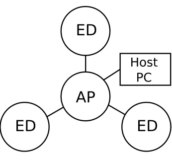
The method used compensates for time offsets between samples and minimizes the effect of clock

drift by periodically synchronizing independent clock sources together. Figure 3 shows an example

system consisting of three end devices (EDs), one access point (AP) and one host computer. All devices have a timer used for time-stamping and synchronization. All events, including samples and

AP

ED

ED

ED

Host

PC

Figure 3: Test Network Layout

value of the timer cannot be altered, it can only be reset to zero. This does not, in any way, affect

the synchronization of devices.

The timer inside theAP can be considered the primary, or global, timer. The goal is to synchro-nize allED, or local, timers with the global timer. Whenever the global timer reaches its maximum value, and rolls over back to zero, theAP sends a broadcast synchronization beacon instructing each end device it is time zero. When anED receives this message, it compares its current timer value to zero, to calculate the clock drift, and resets it to zero. This ensures that allED timers are aligned, which then allows measurements to occur at close to the same time.

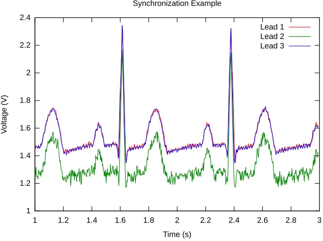
While many, more precise, time synchronization methods are available [9], it was determined

that they were not needed. Due to the low sampling rate and the use of crystal oscillators to run

the timers, the precision obtained with this simple method was good enough for the system. More

complex methods would not have significantly improved results. Figure 4 shows the result of three

separate wireless devices measuring the same signal. This method was used to confirm that the

samples were aligned.

3.5

Scheduling

A round robin-like scheme is used to poll devices in the network. It focuses on simplicity and

portability.

1 1.2 1.4 1.6 1.8 2 2.2 2.4

1 1.2 1.4 1.6 1.8 2 2.2 2.4 2.6 2.8 3

V

oltag

e (

V

)

Time (s) Synchronization Example

Lead 1 Lead 2 Lead 3

Figure 4: Synchronization Test

will wake up when they are scheduled to transmit and send the required data automatically. This

method greatly reduces the power consumption of bothAP and EDs. After initialization, the AP

only needs to send a periodic time synchronization beacon and the collected data back to the host

computer. Once synchronized, end devices will only need to turn their receiver on around the time

the synchronization beacon is expected.

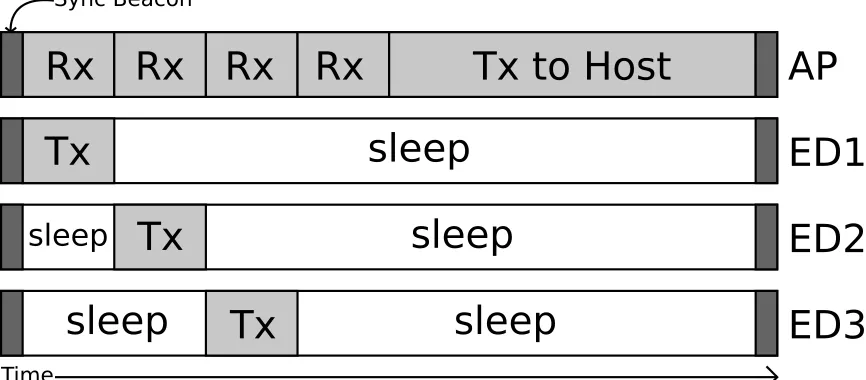
Figure 5 shows a sample system schedule. The figure shows the time each device is on, and the

state of each radio. The “sleep” time for eachED does not show when a device wakes up to sample data. In this specific case, theAP has one extra time-slot allotted for a fourthED.

Certain devices can further reduce power consumption by sampling without using the main

AP

ED1

ED2

ED3

Tx

Tx

Tx

Rx Rx Rx

Tx to Host

Time

sleep

sleep

sleep

sleep

sleep

Rx

Sync Beacon

Figure 5: System Schedule

3.6

Host Interface

The primary focus of this project was to obtain synchronized samples from several wireless devices.

A secondary, but important, goal was to display the data in real time. To speed up development, the

live-plotting tool kst(http://kst-plot.kde.org/) was used. A application, written in C, communicated

via a USB-to-Serial link with the AP and received all of the ED data. It then output the data to

CSV files, which were then used as an input for kst. Figure 6 shows an ECG lead wirelessly measured

from a human subject.

4

Algorithm Development Platform

A platform for testing and analyzing new cost functions for global routing algorithms was developed

in C. The platform allows for a network of nodes and links between the nodes to be created. It

computes the best path from any node to a central source node. Finally, it produces various statistics,

such as energy use, routing maps, and graphical visualizations.

4.1

Initial Development

Initially, the goal of the platform was to test and compare routing with various link costs in an

0.4 0.6 0.8 1 1.2 1.4 1.6 1.8 2

0 0.2 0.4 0.6 0.8 1 1.2

V

oltag

e (

V

)

Time (s) ECG Lead

Lead 1

Figure 6: Sample Measurement from Single ECG Lead

microcontroller and used. This did not turn out to be the case. The first problem encountered

dealt with the network structure used for testing. The program required a list of nodes and a list of

links between the nodes, along with the link costs. Developing a simulated network and links that

accurately represented a real network was unfeasible. The choice was then made to closely couple

the hardware design and the simulator.

4.2

Hardware Coupling

The best way to come up with a network for simulation was to get all of the node and link information

from a real network. The WBAN platform was then used to develop a system for measuring RSSI

data between all nodes in a network. This system allowed for the capture of real network data,

both nodes and links, that could later be used to run routing simulations. The new program

auto-generated a list of nodes, links, and link costs from the previously-measured RSSI data. This new

4.3

Simulation Output

In order to better understand how the new routing system performed, a series of output files were

generated during simulation. The program was set up to account for the energy use of each node

as it routed packets through the network. Visualizing the energy use was vital for the analysis of

network lifetime. Other available data included the routing information itself, which allowed for the

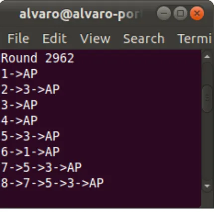
analysis of the routes as the algorithm runs. During run-time, the program prints out text-based

routing information in a terminal window(Figure 8). This provided real-time feedback that was

useful during hardware debugging.

AP 1

-22.7 dBm 2

3

-10.9 dBm

-26.4 dBm

4

-15.6 dBm 5

-13.5 dBm 6

7 -33.9 dBm

-33.9 dBm 8

-25.6 dBm

Figure 7: Sample Network Visualization

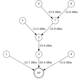
Finally, the program produced a graphical output. The graphical output began as a simple

experiment to see a visual representation of the network. It was later expanded to generate graphs

of the network, and all available connections, as the RSSI data was sampled. Due to the large

number of links between all of the nodes, this graphic was not useful. The final implementation,

which can be seen in Figure 7, only displayed the links used in a specific round of routing. The link

labels display the transmit power required by each node to meet the specific link. The generated

sample video of the generated routing animation can be seen inhttp://www.youtube.com/watch?

v=5Mpn-_FFJaw&hd=1.

Figure 8: Sample Run-time Output

5

Specialized Cost Function for Maximizing Body Area

Net-works Lifetime Using Global Routing Algorithms

5.1

Introduction

There are several routing protocols designed specifically for WBANs. Braem et al. developed

the CICADA protocol, which consists of a spanning tree architecture with a time-division scheme

for transmission scheduling [8]. The primary downside to this method is that nodes closer to the

root will deplete their energy source faster due to the need to relay messages from children nodes.

Other protocols focus on the reliability of the network [12]. Dynamic networks are a problem with

WBANs. If sensors are placed in the extremities, the network will change as the body changes

positions. Quwaider et al. developed a protocol tolerant to network changes [12]. They propose a

store-and-forward method that maximizes the likelihood of a packet reaching its destination. Each

packet is stored by multiple devices and retransmitted, which consumes more power. One solution

nodes with larger power sources. While this method increases the network lifetime, it requires more

hardware. Finally, Nabi et al. propose a similar store-and-forward method, but integrates Transmit

Power Adaptation (TPA) [11]. Nodes keep track of neighbors and use power control to use the

smallest transmit power while maintaining a specific link quality.

In order to provide accurate channel conditions, RSSI measurements of an eight ED network

were used as input to our simulations(5.4). Real-time hardware implementations were also run to

demonstrate the algorithm(5.5). The new cost function succeeded in improving network lifetimes

when run in a dynamic environment. Static environments did not produce successful results.

6

AP

8

7

5

3

4

2

1

α

7,5

C

7,5

7

5

5.2

Proposed Cost Function

In the proposed system, we define a new link cost function that is then used in a routing algorithm.

Traditionally, the power required to make a link possible is used as the link cost. In this case, the

total energy used by a device is factored into the equation. If a device has used more energy than

the others, its use as a relay will be discouraged.

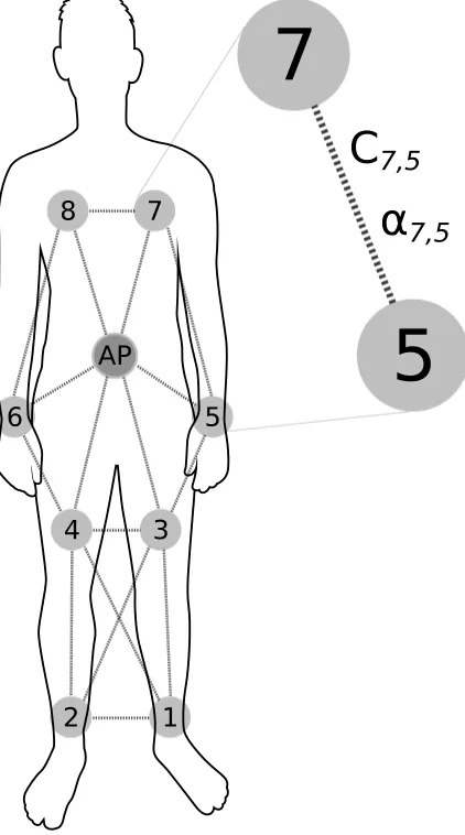
5.2.1 Device Energy

Each device’s normalized energy use is calculated as shown in Equation 2, wherejdenotes the device

ID,iis the current polling round,αj,kis the channel attenuation for the selected link, andRSSIT

is the target RSSI. The current energy used is incremented by the energy used to transmit a single

packet while maintaining RSSIT_{. The channel attenuation for the selected link,α}

j,k, can be seen

in Equation 1, where RSSI is the received power measured by device kand Ptx is the transmitted

power used by devicej.

5.2.2 Link Cost

The actual link cost is computed by calculating the energy used by the device,if that link is selected, and multiplying by a cost factor(Equation 3). The cost factor calculation takes the energy used by

the destination device,E_ik, and divides it by the current energy minimum,E_imin, which is the energy

used by the device with the minimum energy used by roundi. This ratio is then raised to the power

M, which determines how strong the effect will be. If a device’s energy is much greater than the

current minimum, it will be avoided as a relay. TheM factor in Equation 3 can be any number in

0 < M < ∞. The cost factor is normalized so when M = 0, it returns to the traditional cost of

required power to meet the link.

Since the link costs are directly related to the destination device, they are calculated during the

routing algorithm computation. For this paper, Dijkstra’s algorithm [4] is used to select the best

route.

αj,k= RSSI

Ptx

(1)

E₍j_i)=E₍j_i−1)+RSSI

T

C_j,ki =RSSI

T

αj,k

× 

 

1 + Eik Emin

i

M

2





 (3)

5.2.3 Assumptions

This algorithm works under several assumptions. The first being that this is a centralized network

with one Access Point (AP) with virtually unlimited energy and computing power. The second is

that each wireless sensor, or End Device(ED), can act as a relay for messages from other nodes. The

Third is that the link quality, or channel attenuation, between all EDs and AP is known. Finally,

all EDs begin with an equal energy used, that is, they all have the same energy stored. All routing

calculations take place in the AP. Figure 9 shows a sample network with EDs labeled 1 through 8,

and one AP.

5.3

Performance Analysis

In what follows, we analyze the performance of the proposed cost function. The new cost function

was tested in both simulated and experimental environments. In order to gauge the efficiency of the

cost function, it will be compared to an identical system which uses a traditional link cost function.

The traditional link cost function consists of the required power to meet a link with the desired

RSSIT_{. This can be achieved by setting a value ofM = 0 in the new link cost function.}

Performance is determined by the time it takes any node’s accumulated normalized energy to

cross an arbitrary threshold. The threshold could be equivalent to the amount of energy stored in

a device battery, but for this experiment, is purely arbitrary.

5.3.1 Algorithm Implementation

Detailed pseudo-code for the routing algorithm can be found in Algorithm 1. Similarly, code for

energy used calculation can be found in Algorithm 2.

5.4

Simulation

In order to test the new cost function in an efficient manner, a simulation was used. Measurements

of real channel data were acquired by running the procedure described in 5.5.2 without the routing

Algorithm 1Dijkstra’s Algorithm with new cost function

1: fori= 1 to # of Nodesdo

2: nodei.visited←0

3: nodei.distance← ∞

4: nodei.previous←nodei

5: end for

6: nodeAP.distance←0

7: energymin =min(node.energy)

8: while unvisited nodes availabledo

9: nodesource ←node with smallest distance

10: fori= 1 to # of Linksdo

11: if linki.source=nodesource then

12: nodedest←linki.destination

13: if nodedest.visited= 0then

14: cost←linki.power∗(1 +nodedest.energy/energymin)M/2

15: newdistance←nodesource.distance+cost

16: if distance < nodedest.distancethen

17: nodedest.distance←newdistance

18: nodedest.previous←nodesource

19: end if

20: end if

21: end if

22: end for

23: nodesource.visited←1

24: end while

Algorithm 2Energy Used Calculation

1: fori= 1 to # of Nodesdo 2: nodeptr =nodei

3: if nodeptr.previous=nodeptr then

4: No path tonodei

5: else

6: while nodeptr.previous6=nodeptr do

7: linkptr←link betweennodeptr andnodeptr.previous

8: nodeptr.energy+ =linkptr.power

9: nodeptr ←=nodeptr.previous

10: end while

11: end if

12: end for

transmitted it to the host.

Two experimental setups were used to capture RSSI data. For the first, the subject(See Figure 11)

remained relatively static in a sitting position. The second consisted of a more dynamic environment,

where the subject walked around a room as seen in Figure 10.

A set of captured RSSI tables (as seen in Table 1) were fed into the simulation, which proceeded

and routes taken for all devices.

5.5

Hardware Implementation

In order to verify the new cost function in a real environment, a hardware platform was developed

and used. The system function in a similar fashion to the simulation, except that the actual routing

and power control data was fed back to the ED’s.

5.5.1 Hardware Platform

The hardware platform used for this test consists of the Texas Instruments (TI) EZ430-RF2500. This

device includes both an MSP430F2274 microcontroller along with a CC2500 2.4GHz transceiver. The

CC2500 is configured to run at 250kbps. A single device, labeled the Access Point (AP), is connected

via a USB to Serial link, running at 115200 BAUD, to the host computer. All other devices, labeled

End Devices (EDs), are battery powered. In this implementation, the AP acts only as a bridge

between the host and the end devices. All routing and power control calculations are done on the

host.

The host is a laptop computer with an Intel(R) Core(TM) i5-2410M CPU and 4GB of RAM.

Eight EDs were placed on a 170cm, 70kg male subject as shown in Figure 9. The host was carried

on a backpack and connected to the AP via a USB cable. The data was sampled, and the routing

algorithm was run, at a rate of 5Hz. This sampling rate is appropriate as long as the subject, or

its environment, does not move faster than this. If data needs to be sampled at a faster rate, some

hardware and firmware changes might be necessary, but the host software will still work.

For both simulation and hardware experiments, the target RSSI (RSSIT_{) was arbitrarily chosen}

to be−60dBm.

5.5.2 Cycle of Operations

A normal cycle of operations withndevices works as follows:

1: AP sends synchronization beacon which includes routing and power control tables.

2: Each ED transmits its own RSSI table back to the AP, while simultaneously listening to other ED messages and storing the received power from each.

Figure 10: Walking environment.

4: The host uses the RSSI table to compute the routes along with the required powers to meet the selected links.

5: The host sends both routing and power tables back to the AP so that a new cycle may begin.

AP ED1 ED2 ED3 ED4 ED5 ED6 ED7 ED8

AP - -60 -60 -60 -60.5 -60.5 -60.5 -60 -79.5

ED1 -66 - -62 -75 -63.5 -69 -75.5 -73 -67.5

ED2 -72 -61.5 - -80 -69 -70 -74 -75 -66

ED3 -77.5 -74.5 -80.5 - -67.5 -70 -72.5 -70.5 -70

ED4 -39 -63 -69.5 -67 - -82.5 -74.5 -69 -65.5

ED5 -67.5 -68 -71 -69.5 -84 - -55.5 -51.5 -62

ED6 -67 -75 -75 -72.5 -75 -55.5 - -44.5 -53

ED7 -46 -70 -77.5 -70.5 -69 -50.5 -45 - -51.5

ED8 -78 -67.5 -66.5 -71 -66 -62 -54 -51.5

-Table 1: Sample RSSI -Table

5.5.3 Details

To minimize the number of control packets from being transmitted, the EDs are not individually

polled. The only control packet that is sent is the synchronization beacon, which also carries the

schedule to avoid collisions. Each ED has a network ID ranging from 1 to n. The time between

synchronization packets is divided into time-slots than are used by each ED. The time slot used

depends on the network ID of each device. This removes the need to come up with time schedules

during runtime.

The routing table is a simple array which lists the destination for each ED packet. The ED does

not need to know the entire route its packets will take, but only next device in the path. Similarly,

the power table lists the transmit power setting each device needs to use. The size of these tables is

directly proportional to the number of devices in the network.

5.6

Results

Due to the similarities between the simulation and hardware implementation (they both use real

RSSI data), the results were fairly similar. If fed with the same RSSI data, the algorithm will always

produce the same results. The only difference with the hardware implementation is that the RSSI

table is reduced due to the use of power control. Since each ED only uses enough transmit power

to reach a specific ED, others might not receive the message. This was not a problem when the

hardware experiment was run.

0 0.05 0.1 0.15 0.2 0.25 0.3 0.35 0.4

0 50 100 150 200 250 300

A ccum ula te d E ne rgy ( uJ) Time (s)

Accumulated Energy vs. Time (M=0)

ED1 ED2 ED3 ED4 ED5 ED6 ED7 ED8

Figure 12: Sitting M=0

Figures 12 and 13 show the resulting accumulated energies while the subject was in a sitting

position. The experiment was run with both anM = 0 as a reference, andM = 100. Unfortunately,

the results with a static subject were rather neutral. All EDs consume energy at different rates for

both M = 0 and M = 100. A possible explanation for this is that the links between EDs remain

close to the same as time passes. This can become a problem because certain EDs may only have

a single path to choose from. If this is the case, they have no choice but to use the same link

continuously. Not having a choice of paths impairs the ability of the routing algorithm to distribute

0 0.05 0.1 0.15 0.2 0.25 0.3 0.35 0.4

0 50 100 150 200 250 300

A ccum ula te d E ne rgy ( uJ) Time (s)

Accumulated Energy vs. Time (M=100)

ED1 ED2 ED3 ED4 ED5 ED6 ED7 ED8

Figure 13: Sitting M=100

Figures 14 and 15, on the other hand, show an increase in network lifetime. For example, at

the end of the 5 minute sampling run withM = 0, the device which consumed the most power was

ED7 with approximately 1.06 µJ. On the other hand, with M = 100, all EDs consume power in

a uniform fashion and end up with less than 0.81µJ each. One important observation is that the

network withM = 0 consumed less overall power ( 6µJ) than the one withM = 100 ( 6.31µJ). This

is expected, due to the fact that the new cost function specifically avoids the most efficient path

for a specific node in favor of the most efficient path for the whole network. While more energy is

consumed overall, no single ED consumes much more power than others.

Another way of interpreting these results is that energy use in the network is more efficient.

When a single ED depletes its energy source using the traditional link cost, there is a significant

amount of energy left unused in the network. At the same time, when an ED dies in a network using

the new link cost, there should be much less energy left in the rest of the network.

To demonstrate the network lifetime improvement, an ED will be considered have depleted it’s

power source after consuming 0.625 µJ of energy. In the previous example, the trial with M = 0

reaches 0.625µJ after approximately 175 seconds, while the case with M = 100 reaches it around

0 0.2 0.4 0.6 0.8 1 1.2

0 50 100 150 200 250 300

A ccum ula te d E ne rgy ( uJ) Time (s)

Accumulated Energy vs. Time (M=0)

ED1 ED2 ED3 ED4 ED5 ED6 ED7 ED8

Figure 14: Walking M=0

0 0.1 0.2 0.3 0.4 0.5 0.6 0.7 0.8

0 50 100 150 200 250 300

A ccum ula te d E ne rgy ( uJ) Time (s)

Accumulated Energy vs. Time (M=100)

ED1 ED2 ED3 ED4 ED5 ED6 ED7 ED8

A good example of the algorithm working was a result of hardware problems. During of the

experiments, a single ED went off-line for several seconds and was manually restarted. Figure 16

shows the effect the ED failure had on the network. Because a device that is powered off does not

consume power, it became the one with the least energy used. When it returned to the network, it

was immediately used as a relay by other nodes.

0 0.1 0.2 0.3 0.4 0.5 0.6 0.7 0.8 0.9 1

0 100 200 300 400 500 600

A ccum ula te d E ne rgy ( uJ) Time (s)

Accumulated Energy vs. Time (M=100) ED1 ED2 ED3 ED4 ED5 ED6 ED7 ED8

Node Fails

Node Restored

Figure 16: Walking M=100

6

Conclusion

The developed WBAN software libraries were successfully used to implement both the wireless ECG

system and the full-body routing system. The wireless ECG system was able to sample data at a

rate of 300Hz and display in real-time through the host computer. The routing algorithm testing

platform facilitated the development of the new link cost function to maximize network lifetime.

After analyzing the results, the new link cost function successfully improved network lifetime.

The new cost function outperformed the traditional one in trials dealing with a dynamic environment,

where the subject was walking. When the subject was not moving, both link costs performed about

overall power consumption.

While the new link cost was successful, there is room for improvement. One improvement that

can be done deals with the example from Figure 16. While the failed ED was not part of the network,

it was still taken into account when it came to link cost calculation. A better implementation would

not include off-line devices in the calculation. A second modification would relate actual battery,

or other power source, charge to the algorithm. This would allow for devices to join and leave the

network while maintaining proper operation. It would also allow devices with different power sources

to be included and used.

The use of power control, coupled with this new link cost function, should allow WBANs to

run efficiently for long periods of time, while maximizing the network lifetime. Networks requiring

all devices to be on-line to function will greatly benefit from this routing method. Other networks

can also benefit. Due to the normalization of energy use in the network, devices will deplete their

energy sources at similar times. This could be beneficial as all devices can be recharged or replaced

simultaneously, instead of constantly monitoring and replacing individual devices.

References

[1] J. N. Al-Karaki and A. E. Kamal. Routing techniques in wireless sensor networks: a survey.

IEEE Wireless Communications, 11(6):6–28, December 2004.

[2] Geoffrey W. Allen, Konrad Lorincz, Matt Welsh, Omar Marcillo, Jeff Johnson, Mario Ruiz, and

Jonathan Lees. Deploying a Wireless Sensor Network on an Active Volcano. IEEE Internet Computing, 10(2):18–25, March 2006.

[3] Bart Braem, Benoit Latre, Ingrid Moerman, Chris Blondia, and Piet Demeester. The wireless

autonomous spanning tree protocol for multihop wireless body area networks. InThe Wireless Autonomous Spanning tree Protocol for Multihop Wireless Body Area Networks, pages 1–8, July 2006.

[5] Aida Ehyaie, Massoud Hashemi, and Pejman Khadivi. Using relay network to increase life time

in wireless body area sensor networks. InUsing relay network to increase life time in wireless body area sensor networks, pages 1–6, June 2009.

[6] Jeremy Elson, Lewis Girod, and Deborah Estrin. Fine-grained network time synchronization

using reference broadcasts. SIGOPS Oper. Syst. Rev., 36(SI):147–163, December 2002. [7] Saurabh Ganeriwal, Ram Kumar, and Mani B. Srivastava. Timing-sync protocol for sensor

networks. In Proceedings of the 1st international conference on Embedded networked sensor systems, SenSys ’03, pages 138–149, New York, NY, USA, 2003. ACM.

[8] Benoit Latre, Bart Braem, Ingrid Moerman, Chris Blondia, Elisabeth Reusens, Wout Joseph,

and Piet Demeester. A low-delay protocol for multihop wireless body area networks. In A Low-delay Protocol for Multihop Wireless Body Area Networks, pages 1–8, 2007.

[9] Mikl´os Mar´oti, Branislav Kusy, Gyula Simon, and ´Akos L´edeczi. The flooding time

synchro-nization protocol. InProceedings of the 2nd international conference on Embedded networked sensor systems, SenSys ’04, pages 39–49, New York, NY, USA, 2004. ACM.

[10] D. L. Mills. Internet time synchronization: the network time protocol. IEEE Transactions on Communications, 39(10):1482–1493, Oct 1991.

[11] Majid Nabi, Twan Basten, Marc Geilen, Milos Blagojevic, and Teun Hendriks. A robust

protocol stack for multi-hop wireless body area networks with transmit power adaptation . In

BodyNets’10, September 2010.

[12] Muhannad Quwaider and Subir Biswas. On-body packet routing algorithms for body sensor

networks. InOn-body Packet Routing Algorithms for Body Sensor Networks, pages 171–177, 2009.

[13] Adrian Sapio and Gill R. Tsouri. Low-Power body sensor network for wireless ECG based on

relaying of creeping waves at 2.4GHz. InLow-Power Body Sensor Network for Wireless ECG Based on Relaying of Creeping Waves at 2.4GHz, pages 167–173, June 2010.

[14] Thomas Schmid, Prabal Dutta, and Mani B. Srivastava. High-resolution, low-power time

Con-ference on Information Processing in Sensor Networks, IPSN ’10, pages 151–161, New York, NY, USA, 2010. ACM.

[15] Gyula Simon, Mikl´os Mar´oti, ´Akos L´edeczi, Gy¨orgy Balogh, Branislav Kusy, Andr´as N´adas,

G´abor Pap, J´anos Sallai, and Ken Frampton. Sensor network-based countersniper system. In

Proceedings of the 2nd international conference on Embedded networked sensor systems, SenSys ’04, pages 1–12, New York, NY, USA, 2004. ACM.

[16] Philipp Sommer and Roger Wattenhofer. Gradient clock synchronization in wireless sensor

networks. In Proceedings of the 2009 International Conference on Information Processing in Sensor Networks, IPSN ’09, pages 37–48, Washington, DC, USA, 2009. IEEE Computer Society. [17] Makoto Suzuki, Shunsuke Saruwatari, Narito Kurata, Masateru Minami, and Hiroyuki

Morikawa. A quantitative error analysis of synchronized sampling on wireless sensor networks

for earthquake monitoring. In Proceedings of the 6th ACM conference on Embedded network sensor systems, SenSys ’08, pages 417–418, New York, NY, USA, 2008. ACM.

[18] Ning Xu, Sumit Rangwala, Krishna K. Chintalapudi, Deepak Ganesan, Alan Broad, Ramesh