Jacobian-Based Iterative Method for Magnetic Localization in Robotic Capsule Endoscopy

Robotic Capsule Endoscopy

.

White Rose Research Online URL for this paper:

http://eprints.whiterose.ac.uk/103408/

Version: Accepted Version

Article:

Di Natali, C, Beccani, M, Simaan, N et al. (1 more author) (2016) Jacobian-Based Iterative

Method for Magnetic Localization in Robotic Capsule Endoscopy. IEEE Transactions on

Robotics, 32 (2). pp. 327-338. ISSN 1552-3098

https://doi.org/10.1109/TRO.2016.2522433

(c) 2016 IEEE. Personal use of this material is permitted. Permission from IEEE must be

obtained for all other users, including reprinting/ republishing this material for advertising or

promotional purposes, creating new collective works for resale or redistribution to servers

or lists, or reuse of any copyrighted components of this work in other works.

[email protected] https://eprints.whiterose.ac.uk/

Reuse

Unless indicated otherwise, fulltext items are protected by copyright with all rights reserved. The copyright exception in section 29 of the Copyright, Designs and Patents Act 1988 allows the making of a single copy solely for the purpose of non-commercial research or private study within the limits of fair dealing. The publisher or other rights-holder may allow further reproduction and re-use of this version - refer to the White Rose Research Online record for this item. Where records identify the publisher as the copyright holder, users can verify any specific terms of use on the publisher’s website.

Takedown

If you consider content in White Rose Research Online to be in breach of UK law, please notify us by

Jacobian-based Iterative Method For Magnetic

Localization in Robotic Capsule Endoscopy

Christian Di Natali

,

Student Member, IEEE,

Marco Beccani,

Student Member, IEEE,

Nabil Simaan,

Senior Member, IEEE

and Pietro Valdastri,

Senior Member, IEEE

Abstract—The purpose of this study is to validate a Jacobian-based iterative method for real-time localization of magnetically controlled endoscopic capsules. The proposed approach applies finite element solutions to the magnetic field problem and least squares interpolations to obtain closed-form and fast estimates of the magnetic field. By defining a closed-form expression for the Jacobian of the magnetic field relative to changes in the capsule pose, we are able to obtain an iterative localization at a faster computational time when compared with prior works, without suffering from the inaccuracies stemming from dipole assumptions. This new algorithm can be used in conjunction with an absolute localization technique that provides initialization values at a slower refresh rate.

The proposed approach was assessed via simulation and experimental trials, adopting a wireless capsule equipped with a permanent magnet, six magnetic field sensors, and an inertial measurement unit. The overall refresh rate, including sensor data acquisition and wireless communication, was 7 ms, thus enabling closed-loop control strategies for magnetic manipulation running faster than 100 Hz. The average localization error, expressed in cylindrical coordinates, was below 7 mm in both the radial

and axial components, and 5o

in the azimuthal component. The average error for the capsule orientation angles, obtained by

fusing gyroscope and inclinometer measurements, was below 5o

.

I. INTRODUCTION

Wireless capsule endoscopy (WCE) allows physicians to visualize internal organs for diagnosis and potentially for intervention. This paper focuses on creating a modeling and algorithmic framework for localization of magnetically actu-ated WCEs. All the existing platforms for remote magnetic manipulation of a WCE inside the patient’s body operate in open loop [1], i.e. the capsule pose (i.e., position and orien-tation) is not tracked and used for control feedback purposes. Position control of WCEs is typically based on the assumption that the permanent magnet inside the capsule aligns with the external magnetic field. Pose tracking of the WCE would allow the capsule to automatically optimize magnetic coupling to

Research reported in this publication was supported in part by the National Institute of Biomedical Imaging And Bioengineering of the National Institutes of Health under Award Number R01EB018992, and in part by the National Science Foundation under grants CNS-1239355 and IIS-1453129. Any opin-ions, findings and conclusions or recommendations expressed in this material are those of the authors and do not necessarily reflect the views of the NIH or the NSF.Asterisk indicates corresponding author.

C. Di Natali, M. Beccani, and P. Valdastri are with the STORM Lab, Department of Mechanical Engineering, Vanderbilt University, Nashville, TN 37235, USA (e-mail: [email protected]; [email protected]; [email protected]).

N. Simaan is with the ARMA Lab, Department of Mechanical En-gineering, Vanderbilt University, Nashville, TN 37235, USA (e-mail: [email protected]).

maintain effective magnetic actuation, enabling the user to detect if the capsule is not following the expected trajectory (i.e., the capsule is trapped within a tissue fold), and to take appropriate countermeasures for re-establishing an effective motion. An example of position closed-loop control for a magnetically manipulated WCE is presented in [2], where optical tracking with external cameras is adopted to localize the capsule. To apply these results in a clinical setting and move toward the closed-loop manipulation of magnetic WCE position and orientation, online pose tracking without line-of-sight is crucial [3, 4].

Known methods for WCE pose tracking were designed largely for diagnostic purposes (i.e., to associate a lesion visualized by the capsule to its position inside the patient’s body) [5, 6, 7, 8], and are not compatible with magnetic manipulation due to electromagnetic interference with the external source of the driving field. Recently, a number of groups working on robotic magnetic manipulation of WCE began studying localization strategies that are compatible with magnetic manipulation. These works implement localization based on measuring the magnetic field at the WCE via magnetic field sensors. Generally, these works rely on absolute localization using simple dipole models (e.g. [9, 10]) or lookup tables based on finite element solutions to the exact magnetic field (e.g. [11, 3]). The simple dipole models provide limited localization performance when the WCE is close to the mag-netic field source. They work best when the WCE workspace is far away from the driving magnet. However, to maximize the magnetic coupling, the WCE should ideally operate as close as possible to the driving magnet. The drawbacks of lookup table based localization are the slow refresh rate and large memory requirements.

and a position error of 10 mm within a 12 cm workspace. Better performances are obtained in [4], where refresh rate goes down to 30 ms and the error drops below 6 mm within a 15 cm workspace. Finally, in our previous work [4], the sensor data acquisition and the localization algorithm required 6.5 ms and 16 ms per loop, respectively. One of the aims of our proposed new localization method is to decrease computational time, thus achieving both sensor acquisition and localization within 10 ms, allowing the implementation of a 100 Hz WCE manipulation closed-loop control.

In this paper, we validate our proposed algorithm on a WCE localization setup that includes an extracorporeal magnetic field source that manipulates an intracorporeal WCE. The localization strategy proposed herein aims to provide the change in pose of a WCE with respect to an external magnetic field source having known position and orientation. Using a similar approach to that used in [11, 3, 4], the capsule is henceforth assumed to be equipped with an inertial measure-ment unit (IMU) and six orthogonal magnetic field sensors. When inertial data from IMU are integrated, as we propose in our method, drift becomes an issue over time. For this reason, our approach is best used in synergy with an absolute localization technique [3, 4] working at a slower refresh rate. In such a scheme, the absolute localization can repeatedly provide initialization values to our algorithm, thus preventing the integration error from exceeding a desired value.

The contribution of this paper stems from putting forward a new approach for WCE localization by using an iterative Jacobian-based method. To the best of our knowledge, iterative methods for WCE pose tracking that are compatible with magnetic manipulation have not been presented in prior works, partly because a complete analytical solution for the magnetic field is not available. To overcome this challenge, we apply finite element solutions to the magnetic field problem and least squares interpolations to obtain closed-form and fast estimates of the magnetic field. By defining a closed-form expression for the Jacobian of the magnetic field relative to changes in the WCE pose, we are able to obtain an iterative WCE localization method without suffering from the inaccuracies stemming from dipole assumptions and without the downside of a slow refresh rate.

II. METHOD

A. Iterative Method for Magnetic Localization

Our localization approach is inspired by Jacobian-based methods (also known as resolved rates methods stemming from [12]). These methods are commonly used in robotics to solve systems of nonlinear equations subject to the limitations of first-order linearization. In this paper, we assume that the refresh rate for pose tracking is fast enough that only small movements of the WCE may occur between subsequent pose measurements. We also assume that the orientation of the capsule is known through the algorithm described in Section III running on IMU data.

In order to apply an iterative method to magnetic localiza-tion, we need to consider the magnetic field, generated by

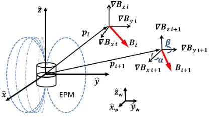
Fig. 1. Schematic representation of the source of magnetic field (External Permanent Magnet (EPM) in figure) and two sequential positions (i.e.,piand

pi+1) of the capsule to be localized. The capsule orientational angles yaw

and pitch are referred to asαandβ, respectively.

a known source, as the following time-invariant non-linear mathematical expression:

B_i=f(p_i) f(p_i) :IR3→IR3. (1)

This equation will be denoted as Magnetic Direct Relationship (MDR). Referring to Fig. 1, the MDR associates the coor-dinates of a point outside the magnetic field source p_i = [xi, yi, zi]T to a corresponding vector function of magnetic

field valuesBi= [Bix, Biy, Biz]T.

If the capsule position changes from pi to pi+1 during a

time increment∆t, the displacement∆pproduces a change in the magnetic field measurements from Bi toBi+1 according

to (1). The partial derivative of the magnetic field vector,

∂

∂pBi, is given by:

∂Bi

∂p =▽pf(pi) =



 

∂B_x ∂px

∂B_x ∂py

∂B_x ∂pz

∂B_y ∂px

∂B_y ∂py

∂B_y ∂pz

∂B_z ∂px

∂B_z ∂py

∂B_z ∂pz





. (2)

where▽pf(pi) designates the gradient off with respect to

p. Using (2) in a first-order Taylor series approximation, we obtain:

B_i+1=Bi+ ∂B_i

∂p∆p=Bi+▽pf(pi)∆p. (3)

The Magnetic Inverse Relationship (MIR), providing the current capsule positionpi+1, can be derived by inverting (3):

pi+1=pi+▽pf−1(pi)∆Bi. (4)

Moving from differential to the finite difference iterative method, ∂_∂pB∆pis replaced by∆Bi, where∆Biis defined as

∆Bi= (Bi+1−Bi). Also, according to [13], the gradient of

a generic vectorial function, which is defined asf(x) :IRn →

IR, is the transpose of the Jacobian as:▽xf(x) = (Jxf(x))t.

Then, (4) becomes:

p_i+1 =pi+J−p1∆Bi, (5)

whereJ−_p1 is the inverse of the Jacobian.

such as Comsol Multiphysics or ANSYS Maxwell. In the next subsections, we introduce a non-linear interpolation method for a data-set of magnetic field values related to the position

pi. Then, the interpolation is used to provide an analytical

expression of the MDR through modal representation, numer-ical algebra theory, and the Kronecker product. Finally, a first order resolved rates method using the Jacobian expression for the MIR is derived.

Figure 2 represents the proposed magnetic localization al-gorithm exploiting sensor fusion of magnetic field and inertial measurements. The magnetic field interpolation (also called magnetic field calibration) is achieved off-line, which leads to obtain the characteristic matrices A_r and A_z. Once the interpolation is obtained, the on-line algorithm takes as input the magnetic field, the inertial measurements, and the External Permanent Magnet (EPM) orientation, returning the capsule pose. The capsule position is referred to the EPM frame, whereas the orientation expressed in Euler angles is relative to the world frame. The blocks DMR-IMR –which stand for Direct and Inverse Magnetic Relationship– and the Iterative Jacobian Method are presented in Section II-B, while the three dimensional reconstruction is presented in Section II-C.

Fig. 2. Block diagram of the proposed iterative algorithm for WCE pose detection. In the diagram are displayed system input, output, Jacobian of the MDR, 3D reconstruction, and the off-line least square fit calibration, which leads to the characteristic matricesAr andAz.

B. Direct and Inverse Magnetic Relationship

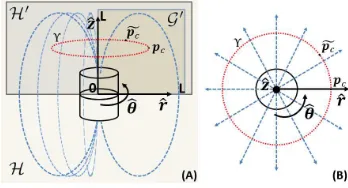
The magnetic field of a cylindrical axially-magnetized permanent magnet exhibits cylindrical symmetry around its main axis (ˆz) [15, 16]. If such a magnet is used as the external source of a magnetic field for capsule manipulation, as suggested in our previous work [3, 4], the localization can take advantage of the symmetry to reduce the computational burden. In particular, the three-dimensional position tracking problem can be reduced to two dimensions (2D). Then, once the position in 2D is obtained, the third coordinate can be derived by sensor fusion as explained in Section II-C.

As represented in Fig. 3, the magnetic field is distributed around the main axis of symmetry of the EPM, ˆz, whileBθ

– angular component of the magnetic field along θ – is null. The vector p˜_c = [r, θ, z]t _{represents a generic point on the}

loci of points, whose location satisfies the condition of having the same magnetic field Bc. This set of points of the locus

generates a circumference Υ(represented in Fig. 3) that can be analytically described as Υ = [r, θ, z]|r, z =const ∈ IR, and θ ∈0 →2π. We refer to p˜c = [r, θ, z]t as the generic

point on the loci, which is expressed in the three cylindrical coordinates, whereas pc lies on the plane Hand is obtained

by applying a rotation aboutˆztop˜c. The planeHis defined

as:H=IR2:{(r, z)|r, z∈IRand θ= 0}.

Considering the magnetic field applied on a generic point p˜_c, its components are expressed as B_c = [Br(r, z), Bθ(r, z), Bz(r, z)], where Bθ(r, z) = 0. Therefore,

(1) could be furthermore simplified by defining the mathemat-ical representationΨfor the magnetic fieldBc. The magnetic

field Bc is given by the two-dimensional transformation Ψ

for any given point p˜c around the magnetic field source,

such as Ψ : ˜pc → Bc. Br(r, z) and Bz(r, z) are two scalar

values representing the radial and the axial component of the magnetic field vector, which are functions of axial and radial spatial coordinates with respect to the center of the EPM.

Fig. 3. Schematic view of the magnetic field distribution for a cylindrical axially-magnetized permanent magnet. (A) View of theHplanes, its subset

H′_{and the domainG}′_{, (B) shows the radial distribution of the magnetic field}

on the plane[ˆr,θˆ].

The solution to the system of equations expressed by the transformationΨ– in terms of both radialBr(r, z)and axial Bz(r, z) magnetic field – is unique in the semi-domain H′

defined as in Fig. 3 (note that the semi-domain H′ _{can be} either related to the south or the north pole of the cylindrical axially-magnetized EPM). Then, we define a finite domain

G′_{, where the magnetic field radial component B}

r is always

positive. On the other hand, if considering the domainH, the transformationΨleads to two solutions in diagonally opposite quadrants in Fig. 3. Since the patient cannot be simultaneously above and below the magnet, we exclude one quadrant for practical implementation reasons. The region is a square plane having sizeLalongˆrandˆz, where the spatial transformation

f(pc)in (1) is simplified and solvable as

Ψ(pc) :IR2→IR2

where:pc∈ G′ :G′={(r, z)∈[0, L]} . (6)

The transformation Ψ(pc)can be expressed by two scalar

mathematical functions, each with two inputs. The two func-tions provide the magnetic field radial component as

Br=ψr(r, z) :IR2→IR, (7)

and the magnetic field axial component as

The numerical solution of (7) and (8) can be obtained by ei-ther applying the Current Density Magnetic Model (CuDMM) or the Charge Density Magnetic Model (ChDMM), as demon-strated in [15, 16]. Then, the magnetic field values can be casted in two data matrices Φr ∈ IRm×p and Φz ∈ IRm×p.

These matrices represent the m×pmagnetic field numerical solutions for any given position pc within G′, where m is

the number of magnetic field measurements taken along theˆr

direction andpis the number of magnetic field measurements taken alongˆz. The collection of numerical solutions[Φr,Φz]T

of (7) and (8), are expressed as in (9) and (10).

Φr= [Φrij(ri, zj)]

i∈IN: [1≤i≥m];j∈IN: [1≤j≥p]. (9)

Φ_z= [Φzij(ri, zj)]

i∈IN: [1≤i≥m];j∈IN: [1≤j≥p]. (10)

whereΦrij andΦzij are the magnetic field values at position

(i, j), which could be generally expressed asΦij. The single

matrix element Φij can be approximated by applying the

modal representation defined in [17, 18, 19] as

Φij =Bi(r, z) =ω(r)Ta(z),

where: (a,ω)∈IRn. (11)

The vector of the modal factors, a(z), can be expressed as

a(z) =Aγ(z),

where: (A,γ)∈IRn. (12)

In this equation, A is the characteristic matrix of coeffi-cients for the particular magnetic field shape, which together with the two orthogonal bases, ω = {ω0, ω1, ..., ωn} and

γ={γ0, γ1, ..., γq}, represents the interpolation functions that

best numerically approximate the transformationΦij over the

domain of interest [20]. Once the interpolation functionsωand

γ are chosen (Section IV-A), and the characteristic matrices of coefficients A_r and A_z for radial and axial magnetic field respectively are derived, the interpolation problem can be easily solved. The best data-set interpolation is chosen by adopting the orthogonal function that minimizes the least square error between the reference measure f(x) and the approximated value y∗_{, such as||f(x)−y}∗_{||< δ. Examples} of orthogonal functions investigated in this study include stan-dard polynomial functions, Chebyshev polynomials [19, 18], Fourier harmonic basis [20, 21] and composition of these.

In the following paragraph, we describe how to derive the characteristic matrices of coefficients Ar and Az for the

algebraic equations system in (11) and (12) by using the following matrix representation, as suggested in [19, 18]:

Φ=Ωm×nAn×qΓq×p, (13)

whereΦ is either the MDR solutions of Φr or Φz within r, z ∈[0→L], whileΩ andΓ are the modal basis matrices and constitute the collection of northogonal basis forΩand

q orthogonal basis for Γ. Finally, m and p are the number of values estimated in the domain r ∈[0, L] andz ∈ [0, L], respectively.

The solutions forAr andAz can be obtained by applying

the Kronecker product theory as in [19, 18, 22], where the symbol⊗represents the Kronecker product of two matrices:

Vec(Φ) = [ΓT ⊗Ω]Vec(A). (14)

The result provided by the algebraic interpolation is the generic matrix of coefficientsA, which is given by

Vec(A) = [ΓT ⊗Ω]†_Vec(Φ),

where:Vec(A) = [a11...an1...an2...anp]T. (15)

Once the matricesAr andAz are known, the MDR, such as ψ(z, y) : (z, y) → (Φij), is solved for any point within the

domainG′_{={(r, z)∈[0, L]}.}

Given the calibration matricesAr andAz, and the

orthog-onal basis ω(r) andγ(z), the system of equation expressed in (11) and (12) is completely determined. By differentiating

ω(r)andγ(z) in∂rand∂z, respectively, we can obtain the complete formulation of the MIR in (2). The following system of equations – expressed for the single solution [Φ_r,Φ_z]T _–

provides the ground to derive the Jacobian:

Φr=ω(r)Arγ(z)

Φz=ω(r)Azγ(z) (16)

Applying (2) to this system of equations, and deriv-ing the partial derivatives of Φ = [Φr,Φz]T such as

∂Φ_r ∂r ,

∂Φ_r ∂z ,

∂Φ_z ∂r ,

∂Φ_z

∂z , the gradient ofΦ becomes

∇Φ=

(

∇Φ_r=∂(ω(r)Arγ(z))

∂r +

∂(ω(r)Arγ(z))

∂z

∇Φz=∂(ω(r) A_zγ(z))

∂r +

(∂ω(r)A_zγ(z)) ∂z

(17)

Considering that the derivatives of the constant coefficient matrices Ar and Az are null, as well as ∂ω_∂z(r) and ∂γ_∂r(z),

(17) simplifies to:

∂Φ_r

∂r =

∂ω(r) ∂r Arγ(z) ∂Φ_r

∂z =ω(r)Ar ∂γ(z)

∂z ∂Φ_z

∂r =

∂ω(r) ∂r Azγ(z) ∂Φ_z

∂z =ω(r)Az ∂γ(z)

∂z

(18)

In order to obtain the expression of ∂ω(r)

∂r and

∂γ(z)

∂z , a

derivation is applied to the vectors constituting the orthogonal basis ω(r), γ(z). This leads to the following expression for the JacobianJΦ:

JΦ=▽p˜cΦ(r, z) =

∂Φr

∂r ∂Φr

∂z ∂Φz

∂r ∂Φz

∂z

(19)

Therefore, the magnetic field vector incremental difference ∆Bi= [∆Br,∆Bz]Ti is given by

∆B_i=

∆Br

∆Bz

i

=JΦ∆pci (20)

This result can be used in (3) to estimate the magnetic field

Bi+1 by continuously updating∆Bi to the current magnetic

field value:

In conclusion, the following equation shows the iterative method to localize the WCE, estimating the current position

pci+1= [ri+1, zi+1]T of the capsule as

pci+1=pci+ ∆pci=pci+J−Φ1∆Bi, (22)

whereJ−1_{is the pseudo-inverse of the Jacobian, which applies}

the least squares method of optimization to the solution [23]. The term ∆Bi is the difference in magnetic field recorded

from the previous measurement.

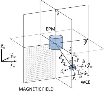
C. Three Dimensional Reconstruction

In order to track the WCE by applying the iterative al-gorithm, both the spatial orientation of the capsule and the external magnetic source pose must be known with respect to a common reference frame. The magnetic field vector Bc

at the capsule position p˜c – expressed in the capsule frame

[ˆx_c,yˆ_c,ˆz_c]– is measured by the onboard sensors. This vector can be expressed in the EPM frame [ˆx,yˆ,ˆz] by applying the geometrical transformationREP M

c , thus obtainingB.

Then, considering Figs. 1 and 3, the magnetic field vector

B is expressed in cylindrical coordinates from its cartesian coordinates, such as:B= [Bx, By, Bz]T →[Br, Bz]T and θ,

whereθcorrespond to the azimuthal coordinate of the capsule positionp˜c. The relationships that transform the magnetic field

vector Bc = [Bxxˆ, Byyˆ, Bzˆz] from cartesian to cylindrical

coordinates are:

Br= q

(Bxxˆ)2+ (Byyˆ)2 ˆr

B_z=Bzˆz

θ=atan2(By, Bx)ˆθ

(23)

where Bx, By, Bz are the cartesian components of the

mag-netic field vector B with respect to the EPM frame [ˆx,ˆy,ˆz]. The axial and radial magnetic field components can be fed into the iterative algorithm, which derives the radial and axial coordinates of the capsulepc= [pr, pz]. These can be used in

combination with θ to derive the three cartesian coordinates as follows:

px=prcos(θ)ˆx

py=prsin(θ)ˆy

pz=pzˆz

(24)

III. CAPSULEORIENTATIONALGORITHM

This section presents the algorithm used to detect the change in capsule orientation and to generate the rotational matrix

Rc with respect to the global frame. This algorithm based on

the fusion of inclinometer and gyroscope outputs is widely adopted in literature and is provided here for the sake of completeness. The capsule orientation knowledge is required in our magnetic localization approach in order to express the magnetic field vector Bc in the EPM frame.

Referring to Fig. 1, the accelerometer can be used as an inclinometer to obtain the absolute values of the two orientational angles α and β [24]. The rotations about x_c

and y_c are derived directly from the gravitational vector g

projection mapped on the three orthogonal axes of the onboard accelerometer as

α=atan2(ay, p

a2 x+a2z)

β=atan2(ax, q

a2 y+a2z)

(25)

whereax, ay, az are the three accelerometer outputs.

A number of methods for inertial navigation can be adopted to estimate the third orientation angleγ, which is the rotational angle along the gravitational vector g. Examples span from fusing gyroscope and inclinometer measurements [25, 26] to applying a quaternion-based algorithm to inertial data [27]. The approach we have adopted involves applying the axis-angle method for rotational matrices to the gyroscope outputs [28]. Briefly, it is possible to extract the rotation γ about the global axis z_w by building the rotational matrix ∆R_c

with respect to the moving frame attached to the capsule [ˆxc,yˆc,ˆzc]. The instantaneous variations in capsule orientation

can be derived from the gyroscope outputs as

∆αc=gx∆t ∆βc =gy∆t ∆γc=gz∆t (26)

where ∆[αc, βc, γc] are the instantaneous angle variations at

the capsule moving frame within a measurement loop that lasts ∆t. The instantaneous capsule rotational matrix∆Rc is then

defined as

∆Rc=Rx(∆αc)Ry(∆βc)Rz(∆γc) (27)

whereRx,Ry,Rz are the rotational matrixes with respect to

the xc, yc, and zc axis, respectively. Then, the axial-angle

representation of the rotational matrix ∆Rc is derived, thus

achieving the angle of rotationθ and the axis of rotationω:

θ=arccostrace(∆Rc)−1

2

ω= _2sin1_(θ)P3_j=1 ˆecj,i׈ecj,i+1

(28)

where ˆe_cj,i and ˆe_cj,i+1 are the unit vectors of the capsule

frame at thei-thand(i+1)-th iterations, respectively. Finally, the axis-angle representationθ,ωmust be reoriented according to the capsule orientation with respect to the global frame at the previous time step,Rt−1

c . The third coordinate of the

axial-angle representation corresponds to the capsule axial-angle variation ∆γ about ˆzw. The capsule absolute orientation γ about the

global axisˆzwis achieved by summation of∆γ at each loop.

IV. SIMULATION-BASEDVALIDATION

A. Magnetic Direct Relationship

Comsol Multiphysics was also used to create the 15×15 matrixΦ_rand the18×18matrixΦ_zrelative to the radial and axial components of the magnetic field, respectively. These two matrices were interpolated using two vectors of modal basis functionsω andγ. The vectorω captures variations of the magnetic field as a function of radial distance rand it is given by:

ω(r) =h1/2,cosπr

L

,sinπr

L

, . . .

. . . ,cos

_π12r

L

,sin

_π12r

L

, r, r2, . . . , r5 (29)

Similarly, the dependence of the magnetic field on variations of the axial component zis captured byγ(z):

γ(z) =h1/2,cosπz

L

,sinπz

L

, . . .

. . . ,cos

_π12z

L

,sin

_π12z

L

, z, z2, . . . , z5 (30)

The modal basis functions were chosen based on simulation of the approximation residue with the minimum number of terms that provide a relative error of less than 10% within a portion of at least 70% of the domain G′_.

BothA_randA_zwere derived applying (15), thus obtaining 31×31matrices. The interpolation was obtained by applying (11) and (12) to any radial and axial coordinate of the domain

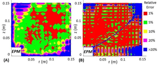
G′_{. The interpolation error was evaluated by comparing the} in-terpolated magnetic field with the reference values derived by Comsol Multiphysics. Given the position vector pci= [r, z]Ti

within G′_{, Fig. 4-a shows the module of the relative error for} the radial magnetic field component, while Fig. 4-b shows the module of the relative error for the axial component. Table I reports the portions of G′ _{where the interpolation error is} below 1%, 5%, 10%, and 20% for both the axial and the radial component of the magnetic field. The radial component estimation presents a relative error below 10% for the 86% of the radial magnetic field map. The axial component estimation shows that the 70% of the axial magnetic field map presents a relative error below 10%. Whenever the value of magnetic field intensity is very small, or null, a small approximation noise leads to a high relative error, as it is shown in Fig. 4. These results show an efficient estimation of bothBrandBz,

thus allowing the MDR to be analytically derived via (16).

Fig. 4. Relative error for the radial (A) and axial (B) magnetic field estimated by the MDR withinG′_.

Fig. 5 shows the ratio of the relative error of the single dipole model [29] to the relative error of our interpolation

method, where the relative error is calculated with respect to the reference values derived by Comsol Multiphysics. The blue regions –ratio between 0 and 1– of the maps correspond to a similar or better performance of interpolation for the dipole model comparing with the proposed method. The dark red regions correspond to ratio greater than 8. Table I reports the portions ofG′ _{where the interpolation error of the dipole} model is below 1%, 5%, 10%, and 20% for both the axial and the radial component of the magnetic field. From these results, we can conclude that the proposed approach provides a more accurate approximation for the magnetic field in both components.

Fig. 5. The ratio of relative errors of the single dipole model to the interpolation model for the radial (A) and axial (B) magnetic field components. Black regions stem from visualization artifacts due to oscillations in the ratio from 3 to 8 times.

Fig. 6. Simulated motion of a capsule along a spiral trajectory in the center ofG′_{. The black line represents the reference trajectory, while the crossed line}

shows the capsule position estimated by applying the Jacobian-based iterative method. The cyan ellipses represent the ellipsoid of localization uncertainty due to magnetic field sensor noise. Colors in the crossed line express the relative error in position detection for the radial component.

B. Magnetic Inverse Relationship

The pose detection iterative method based on (22) was assessed by simulating the capsule motion along a spiral path, starting from a central position in the map pc ≈

TABLE I

PORTIONS OFG′_{SHOWING DIFFERENT LEVELS OF RELATIVE ERROR IN} THE INTERPOLATED MAGNETIC FIELD FROM THE PROPOSED METHOD AND

THE SINGLE MAGNETIC DIPOLE MODEL.

Level of relative error Radial Component Axial Component

Below 1% 42% 30%

Below 5% 78% 61%

Below 10% 86% 70%

Below 20% 92% 79%

Magnetic dipole model Radial Component Axial Component

Below 1% 12% 0.4%

Below 5% 63% 2%

Below 10% 81% 5%

Below 20% 90% 10%

and its pose estimation. The color map represents the relative error of the radial coordinate. The estimation of the simulated capsule pose results in an axial coordinate relative error below 1%, with respect to its current position, for almost the entire simulation. The radial coordinate relative error is below1%for the upper-right, lower-left and lower-right quadrants of the spi-ral path represented in Fig. 6. The upper-left quadrant presents a relative error below 5%. This increased error is related to the radial localization error map of Fig. 4.A. Since the center of the spiral is at the upper left quadrant of Fig. 4.A, where the radial error increases with proximity to the top left corner, the error of localization along the spiral exhibits a similar trend. Also, considering the noise of magnetic field sensor readings, the outcome of the localization algorithm for each capsule position is represented by an ellipsoid of uncertainty (in cyan in Fig. 6). In this simulation, we used the noise levels of ±0.08mT and±0.05mT in measuring Br andBz based

on experimental characterization from the platform described in Section V-A. This simulation demonstrates an average sub-millimeter localization accuracy for both the radial and axial component.

V. EXPERIMENTALASSESSMENT A. Experimental Platform

1) Hardware: The experimental platform, represented in Fig. 7.A, is composed of the WCE, the EPM, a robotic manipulator (RM), and a personal computer (PC) connected to a wireless transceiver via the universal serial bus (USB) port. The real-time algorithm runs on the PC and communicates with the capsule through a USB transceiver. The EPM is an NdFeB (magnetization N52, magnetic remanence 1.48 T) cylindrical permanent magnet with axial magnetization. The EPM diameter and length are both equal to 50 mm, while the mass is 772 g. A six-DOF robot (RV6SDL, Mitsubishi Corp., Japan) mounts at its end-effector the EPM. The robot is controlled in real time through a multi-thread C++ soft-ware application, which is described in section V-A3. The manipulator is used to control and track the EPM position and orientation with respect to the global reference frame [ˆxw,yˆw,ˆzw], which is assumed to be superimposed on the

manipulator ground frame[ˆx0,yˆ0,ˆz0]. The current EPM pose

for the localization algorithm is derived from the robot end-effector pose, which is available at the application interface

level with a resolution of 2×10−2_{mm in position and 1×10}−3

degree in orientation. The EPM orientation frame[ˆx,yˆ,ˆz] is an input for the localization algorithm (as described in section II-C), while the EPM pose, as acquired by the robot encoders, is used as a reference position for the experimental assessment. A load cell (MINI 45, ATI Industrial Automation, USA), mounted in between the EPM and the RM, allows the EPM to be moved via admittance control for the general assessment described in Section V-B5.

Fig. 7. Experimental platform: a) Robotic Manipulator (RM) and External Permanent Magnet (EPM). b) Visual rendering of the Wireless Capsule Endoscope (WCE) and its internal components, where FMSM is the Force and Motion Sensing Module, WMC is the Wireless MicroController and PS is the Power Supply.

Fig. 8. Schematic representation of the global frame, EPM frame and capsule frame. The capsule orientation angles[α, β, γ]are shown with respect the global frame.

2) Wireless Capsule: The WCE, schematically represented in Fig. 7.B, hosts the Force and Motion Sensing Module (FMSM), which was presented in [4], Wireless MicroCon-troller (WMC), and Power Supply (PS). The outer shell is fabricated in VeroWhite 3D printer material (OBJET 30, Stratasys, USA). The current prototype is 36 mm in length, 17.5 mm in diameter, and 15 g in mass. The capsule shell has four lateral wings that are used as a reference to achieve a precise alignment for the capsule frame[ˆxc,ˆyc,ˆzc]during the

calibration.

Mea-surement Unit (IMU) embedding both an accelerometer and a gyroscope (LSM 330, STMicroelectronics, Switzerland), and an off-the-shelf NdFeB (N52) cylindrical magnet, which was axially magnetized with 1.48 T of magnetic remanence, 11 mm in diameter and 11 mm in height. The readings of the magnetic sensors integrated in the FMSM are acquired by the onboard 16-bit Analog to Digital Converter (ADC, AD7689, Analog Devices, Inc. USA). An acquisition cycle starts from sampling six analog inputs connected to the MFS outputs. Then, the six digitized values of acceleration and angular speed are received from the IMU. This dataset is acquired every 4.4 ms by the WMC (CC2530, Texas Instruments, USA) and used to build a 36-byte package together with the capsule status indicators (i.e., battery level, start/stop bytes). This package is then transmitted by the WMC to the external transceiver over a 2.4 GHz carrier frequency, with a refresh time of 6 ms (wireless data throughput 42.4 kbit/s), resulting in a sampling rate of 166 Hz. The external transceiver is based on an identical WMC which communicates with the PC through a USB-serial converter (UM232R, FTDI, UK).

The power supply module embeds a low-dropout voltage regulator (LDO) (TPS73xx, Texas Instruments, USA) to pro-vide a stable supply to both the FMSM and the communication module. In order to limit the current consumption when the device is not acquiring measurements, a digital output of the microcontroller can drive the SLEEP pin of all the MFS. This results in a current consumption which varies between 400 mA, when the microcontroller is in low power mode, and 20 mA when it is in IDLE mode with the radio active. Average current consumption rises to 48 mA during a single cycle of sensor data acquisition and wireless transmission. The power source used is a 50 mAh, 3.7 V rechargeable LiPo battery (Shenzhen Hondark Electronics Co., Ltd., China).

3) Software Architecture: A multi-thread C++ WIN32 ap-plication running on the PC unbundles the data and shares them with three other parallel threads. The first thread controls the robotic manipulator through a UDP/IP communication with a refresh rate of 140 Hz. It sends the desired pose to the robot controller and then receives the robot pose feedback. The second thread implements a digital Kalman filter for each of the six MFS and the six IMU outputs before running the iterative localization algorithm. The algorithm outputs the 6-DOF capsule pose estimationp= [x, y, z, α, β, γ]with respect to the EPM frame[ˆx,yˆ,ˆz]. The third thread manages a TCP/IP communication with a MATLAB application (Mathworks, USA), which displays the localization algorithm estimation. The data transfer rate for the robot controller applications is 83 Hz. The refresh time for the capsule pose estimationpand the capsule wireless data transfer is 6.8 ms (refresh rate 150 Hz). Referring to Fig. 8, the MATLAB application displays the capsule position and orientationp= [x, y, z, α, β, γ]with respect to the EPM reference frame [ˆx,yˆ,ˆz] in real time (refresh every 30 ms) on a 3D plot. Current pose numerical values are also displayed.

B. Experiments and Results

1) Capsule orientation algorithm assessment: Because the localization method we propose also relies on real-time

cap-sule orientation data, the first step in the experimental assess-ment consisted in validating the algorithm described in section III. In order to quantify the absolute error in capsule orienta-tion, the WCE was rigidly attached to the end effector of the RM. The orientation of the WCE was varied within a range of

±90o_{about each of the three axes [x}

EP M, yEP M, zEP M] by

adopting combined motions for a total of one minute. Inertial data acquired by the WCE were sent over the wireless link, while the orientation of the end effector, as measured by the RM built-in encoders, was adopted as a reference. The average orientation error was 3.4o±3.2o_{forα, 3.7}o_±3.5o_{forβ, and}

3.6o±2.6o _forγ.

A second experiment aimed to quantify the steady-state drift for the capsule orientation algorithm. This is particularly relevant for the estimation of γ, which, unlike α and β, is obtained by iterative integration. For this test, the WCE was locked into the capsule dock (see Fig. 7 or the multimedia attachment 1) for 7.5 minutes while acquiring data and running the capsule orientation algorithm. The average error and its standard deviation over the entire period was 0.34o±0.18o

for α, 0.27o±0.17o _{for β, and 1.8}o_±1.1o _{for γ, while the}

absolute error at the end of the 7.5 minutes was 0.5o for α, 0.2o forβ, and 5.2o forγ.

2) Steady state positional drift evaluation: This set of experiments, referred to as T01, was aimed at evaluating the localization algorithm behavior in steady conditions. Before the trials began, the iterative localization algorithm was initial-ized as shown in the multimedia attachment 1. The calibration consisted of three steps. First, the capsule was placed into the capsule dock, with a known position and orientation with respect to the global frame [xw, yw, zw]. Then, the magnetic

field sensors in the WCE were biased while maintaining the EPM outside the workspace. Finally, the EPM was moved to a reference position with respect to the WCE, and the relative distance between the EPM and the WCE, as derived by design, was used to initialize p(t = 0) (digitization phase in the multimedia attachment 1).

After the initial calibration, the EPM was moved to eight different positions within the workspace, while the WCE was maintained in the capsule dock. Each position was chosen to be at about 10 cm from the center of the workspace along both the radial and axial coordinate. The radial and axial coordinates of the EPM were fixed to 80 mm and 130 mm, respectively. The azimuth coordinateθEP M was changed from

zero to2πin π/4 steps. Each EPM position was maintained for one minute, while recording the localization data. The results were compared to the reference EPM pose as derived by the RM encoders. Table II reports the azimuth coordinate, the average radial error and the average axial error for each of the eight EPM positions.

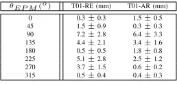
TABLE II

RESULTS OF THE STEADY STATE POSITIONAL DRIFT EXPERIMENT(T01).

θEP M(o) T01-RE (mm) T01-AR (mm) 0 0.3±0.3 1.5±0.5 45 1.5±0.9 0.3±0.3 90 7.2±2.8 6.4±3.3 135 4.4±2.1 3.4±1.6 180 0.5±0.5 1.8±0.8 225 5.1±2.8 2.5±1.2 270 3.7±1.5 0.6±0.2 315 0.5±0.4 0.4±0.3

Typical trends for radial and axial component estimation are shown in Fig. 9. During the trials, the pose estimation presented a drift due to the system noise and the iterative integration. However, the relative error was always below5%. The residual measurement noise (Fig. 9.d) had a gaussian distribution (Jarque-Bera normality test with h equal to 1 and p-value 0.1) with null average and a bandwidth below 0.5%, which remained constant for the entire duration of each trial. The magnetic field measurement noise fused with the IMU measurements did not affect the localization algorithm, thus resulting in a stable long-term behavior.

Fig. 9. Results for the steady state positional drift experiment (T01) and for the initialization error evaluation (T02) with an initialization error of10mm. Both T01 and T02 results are evaluated for the radial (left column) and the axial (right column) component. (a) Reference position vs. estimation. (b) Absolute positional errors. (c) Relative positional errors. (d) Residual measurement noise. The azimuth error is presented in Fig. 12.

3) Robustness to initialization errors: This set of experi-ments, referred to as T02, was aimed at assessing the algorithm sensitivity to errors in position initialization. These trials were performed by moving the EPM to the same eight positions used for T01, while maintaining the WCE fixed into the capsule dock. For each EPM position, four different tests were performed by adding an increasing erroreto the initialization

distancep(t= 0)as measured during calibration. In particular, the errorehad a random direction inˆrandˆzand an increasing module (i.e., 1 mm, 5 mm, 10 mm, and 20 mm). As in T01, each test was one minute long.

Considering all 32 tests performed, the average absolute and relative error for the radial component were15.5±4.2mmand 19.5±6.0%, respectively. The axial component had an average absolute error of 13.6±3.9mmand an average relative error of 12.1±3.5%.

Typical trends for radial and axial component estimation affected by a 10 mm error in position initialization are shown in Fig. 9. In this case, the absolute and the relative error (Fig. 9.b and Fig. 9.c, respectively) decreased within the duration of the trial, never exceeding 10% of the reference value. Interestingly, the localization algorithm was able to correct the initialization error with time. The residual measurement noise for both the radial and the axial component (Fig. 9.d) presented the same behavior observed in T01 trials.

4) Robustness to positional lag: This set of trials aimed at evaluating the effect that a lag between the EPM and the WCE may have on the localization algorithm. In particular, our goal was to quantify the minimum value for the relative speed between the EPM and the WCE that would prevent the localization algorithm to converge. For reference, the typical endoscope absolute speed during a colonoscopy is in the order of 0.8 mm/s to 1.6 mm/s [30]. However, for magnetic capsule endoscopy, the relative EPM-WCE speed is ideally null, as the WCE should be following the EPM motion under the effect of magnetic coupling. This is true as long as the WCE is able to freely move inside the lumen.

After the initial calibration as described for T01, five trials were performed by moving the EPM at increasing speeds while collecting localization data. Like the previous experi-ments, the WCE was locked into the capsule dock. The EPM was initially positioned at 110 mm along the radial component and 110 mm along the axial component, and then moved by 200 mm alongywat a constant acceleration. For the five trials,

acceleration was set to 0.396,0.793,1.190,1.587, and 1.984

m

s2, respectively. The multimedia extension 1 shows one of

these trials, while the results for the experiment with 1.984

m

s2 acceleration are reported in Fig. 10. As expected, the EPM

motion along yw only affected the radial component of the

localization algorithm, leaving the axial component almost unperturbed.

For this set of trials, the localization algorithm presented a relative error in the radial component of 10% for a relative speed of 0.221±0.046 m

s. This increased up to20% for a

relative speed of0.335±0.050 m

s. The average absolute error

in the radial component was11.86±8.36mm, with an average relative error of 16.3±10.2%. For the axial component, the average absolute error was 2.66±1.8mm, with an average relative error of2.3±1.6%.

Given these results, we can conclude that the algorithm is sensitive to the relative speed between the WCE and the EPM and the relative error exceeds 10% if the relative speed is greater than0.2m

s. As previously discussed, this speed is well

Fig. 10. Position estimation results during the positional lag trial with uniform acceleration of1.984 m

s2.

5) General assessment: The final experiment aimed at validating the localization algorithm for a generic trajectory of the EPM, with the WCE fixed into the capsule dock. After calibration, the EPM was moved via admittance control to form a three-dimensional loop within the workspace, starting from the initialization positionp(t= 0). During this trial, the EPM coordinates spanned from about -10cmto 10cmalong both xˆw and yˆw axes, and from 6 cmto 12 cm away from

the WCE position along the ˆz_w axis.

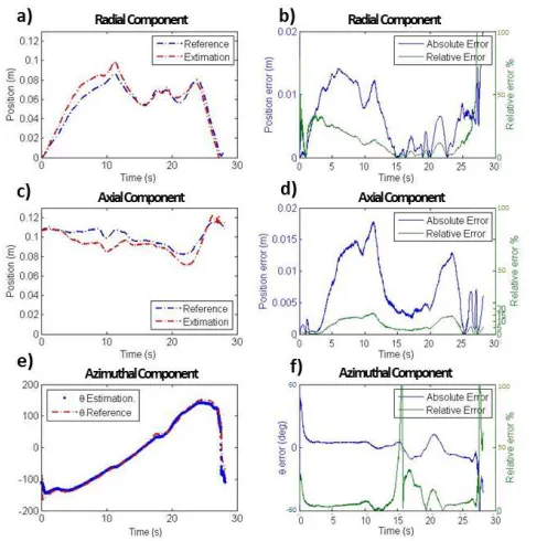
For the entire trajectory, the proposed method of localization presented an average absolute error in the radial component of 6.2±4.4mm and an average relative error of5.7±7.6%. The average absolute error for the axial component was6.9±

3.9mm, with an average relative error of 7.0±4.9%. The average absolute error for the azimuth component (θ) was 5.4o_±7.9o_.

The trajectory (as reconstructed from the RM encoders) and its estimation are represented in Fig. 11. Typical trends for the radial (r), the axial (z), and the azimuthal (θ) component estimations are shown in Fig. 12.a,c,e, while the absolute and relative errors are reported in Fig. 12.b,d,f. The azimuthal component presents a large absolute error when the radial component of the capsule position is approaching zero. This is due to minor misalignments between the capsule and the EPM. This error is significantly attenuated in the conversion of the pose from cylindrical to Cartesian coordinates by applying (24), as the radial componentpris very small or equal to zero.

It is worth noting that the experimental assessment showed an error that is about one order of magnitude larger than what was observed by simulation. This is probably due to the noise introduced by the sensors and by the digitization process.

Real-time operation of the localization algorithm for random motion of the WCE is shown in the multimedia extension 2. On the left side of the screen, the localization output is plotted in real-time showing the WCE and the EPM reference frames. In the multimedia extension 3, the localization is performed while moving the EPM parallel to a plexiglass pipe placed at an angle with respect to the global frame. In this case, the WCE is free to move in the pipe under the effect of magnetic coupling. The distance between the EPM and the WCE is about 10 cm. The localization real-time output p= [x, y, z, α, β, γ] and the EPM position are both superimposed to the video stream. This demonstrates the ability of the proposed localization algorithm to track the WCE in real-time

Fig. 11. Three-dimensional representation of the EPM trajectory and its estimation by the localization algorithm.

Fig. 12. Typical trends for the radial (a), the axial (c) and the azimuth (e) component during the final experiment, and related absolute and relative errors (b, d, and f, respectively).

during magnetic manipulation.

VI. CONCLUSIONS

used Kronecker products and a modal fitting to describe the magnetic field. To assist with real-time localization (which is paramount for solving a nonlinear inverse problem), we used the Jacobian of the magnetic field intensity relative to pose perturbations of the endoscopic capsule. This allowed the use of a local linearization approach that is similar to the resolved rates method for inverse kinematics of serial robots.

Our algorithm was evaluated by simulation and experiments. We investigated the robustness of our pose estimates of the wireless capsule to initialization errors. We also characterized the residual measurement noise and the effect of positional lag when the magnet driving the capsule was moving. Our results showed that, even though the proposed algorithm exhibits limitations of convergence for fast relative motions, the pose estimation of the magnetic capsule for clinically realistic speeds was effective and reliable. In particular, experimental results showed an average error (expressed in cylindrical coor-dinates) below 7 mm in both the radial and axial components, and 5o in the azimuthal component. The average errors for the capsule orientation angles, obtained by fusing gyroscope and inclinometer measurements, were 0.3o for αand β, and 5o for γ. Overall, the relative error always remained below 10%. The proposed localization algorithm was able to run at a 1 ms refresh rate, an order of magnitude below what was reported in previous works. The overall refresh rate, including sensor data acquisition and wireless communication, was 7 ms, thus enabling closed-loop control strategies for WCE magnetic manipulation running faster than 100 Hz. Since the least square interpolation present some regions of the magnetic field domainG′ _{where the relative error is greater than 20%, in} future applications the robot path planner can be instructed to follow the capsule and to enclose it in an optimal localization area to avoid these regions.

Drift – a common problem in integrative methods – may become an issue over time and affect the precision of localiza-tion. A possible solution is to integrate the proposed approach with absolute localization strategies [3, 4] or with techniques fusing multiple sensor data having different resolutions and refresh rates, as proposed in [31, 32, 33] for SLAM appli-cations. Since the final goal is to localize the capsule during magnetic manipulation, the behaviour of the algorithm must be quantitatively assessed with the capsule in motion against a reference localization method (i.e., vision-based localization as in [2]), exploiting also inertial navigation system theory by applying the extended Kalman filter [34, 35].

In summary, the proposed localization strategy is compatible with magnetic manipulation of WCE, does not require clear line-of-sight, has a resolution that is finer than the capsule size, and a refresh rate that is adequate for real-time closed loop robotic control. This represents an enabling technology that can move us toward intelligent control of a WCE during an endoscopic procedure.

REFERENCES

[1] P. Valdastri, M. Simi, and R. J. Webster III, “Advanced technologies for gastrointestinal endoscopy,”Annual Re-view of Biomedical Engineering, vol. 14, pp. 397–429, 2012.

[2] A. W. Mahoney and J. J. Abbott, “Five-degree-of-freedom manipulation of an untethered magnetic device in fluid using a single permanent magnet with applica-tion in stomach capsule endoscopy,” The International Journal of Robotics Research, 2015, in press, available on-line.

[3] C. Di Natali, M. Beccani, and P. Valdastri, “Real-time pose detection for magnetic medical devices,” IEEE Trans. Magn., vol. 49, no. 7, pp. 3524–3527, 2013. [4] C. Di Natali, M. Beccani, K. Obstein, and P. Valdastri, “A

wireless platform for in vivo measurement of resistance properties of the gastrointestinal tract,” Physiological measurement, vol. 35, no. 7, p. 1197, 2014.

[5] T. D. Than, G. Alici, H. Zhou, and W. Li, “A Review of Localization Systems for Robotic Endoscopic Capsules.” IEEE Trans. Bio-Med. Eng., vol. 59, no. 9, pp. 2387– 2399, 2012.

[6] C. Hu, M. Li, S. Song, R. Zhang, M.-H. Menget al., “A cubic 3-axis magnetic sensor array for wirelessly tracking magnet position and orientation,”Sensors Journal, IEEE, vol. 10, no. 5, pp. 903–913, 2010.

[7] S. Song, B. Li, W. Qiao, C. Hu, H. Ren, H. Yu, Q. Zhang, M. Q.-H. Meng, and G. Xu, “6-d magnetic localization and orientation method for an annular magnet based on a closed-form analytical model,” Magnetics, IEEE Transactions on, vol. 50, no. 9, pp. 1–11, 2014. [8] D. M. Pham and S. M. Aziz, “A real-time localization

system for an endoscopic capsule,” inIntelligent Sensors, Sensor Networks and Information Processing (ISSNIP), 2014 IEEE Ninth International Conference on. IEEE, 2014, pp. 1–6.

[9] K. M. Popek, A. W. Mahoney, and J. J. Abbott, “Lo-calization method for a magnetic capsule endoscope propelled by a rotating magnetic dipole field,” inRobotics and Automation (ICRA), 2013 IEEE International Con-ference on. IEEE, 2013, pp. 5348–5353.

[10] S. Yim and M. Sitti, “3-d localization method for a magnetically actuated soft capsule endoscope and its applications,” Robotics, IEEE Transactions on, vol. 29, no. 5, pp. 1139–1151, 2013.

[11] M. Salerno, R. Rizzo, E. Sinibaldi, and A. Menciassi, “Force calculation for localized magnetic driven capsule endoscopes,” in Robotics and Automation (ICRA), 2013 IEEE International Conference on, 2013, pp. 5354–5359. [12] D. Whitney, “Resolved Motion Rate Control of Manip-ulators and Human Prostheses,” IEEE Transactions on Man Machine Systems, vol. 10, no. 2, pp. 47–53, Jun. 1969.

[13] J. Nocedal and S. J. Wright, Numerical Optimization, T. V. Mikosh, S. M. Robinson, and S. Resnick, Eds. Springer, 2006.

[14] E. P. Furlani,Permanent Magnet and Electromechanical Devices. Elsevier, 2001, pp. 131–135.

[15] ——,Permanent magnet and electromechanical devices [electronic resource]: materials, analysis, and applica-tions. Access Online via Elsevier, 2001.

Mag-netics, IEEE Transactions on, vol. 33, no. 3, pp. 2322– 2325, 1997.

[17] G. S. Chirikjian and J. W. Burdick, “A Modal Ap-proach to Hyper-Redundant Manipulator Kinematics,” IEEE Transactions on Robotics and Automation, vol. 10, no. 3, pp. 343–354, 1994.

[18] J. Zhang, K. Xu, N. Simaan, and S. Manolidis, “A pilot study of robot-assisted cochlear implant surgery using steerable electrode arrays,” in Medical Image Comput-ing and Computer-Assisted Intervention–MICCAI 2006. Springer, 2006, pp. 33–40.

[19] J. Zhang, J. T. Roland, S. Manolidis, and N. Simaan, “Optimal path planning for robotic insertion of steerable electrode arrays in cochlear implant surgery,”Journal of medical devices, vol. 3, no. 1, 2009.

[20] H. F. Davis, Fourier series and orthogonal functions. DoverPublications. com, 1963.

[21] N. Csanyi and C. K. Toth, “Some aspects of using Fourier analysis to support surface modeling,” inProceedings of Pecora 16, Global Priorities in Land Remote Sensing, Sioux Falls, South Dakota, October 2005, pp. 1–12. [22] J. Brewer, “Kronecker products and matrix calculus in

system theory,”Circuits and Systems, IEEE Transactions on, vol. 25, no. 9, pp. 772–781, 1978.

[23] P. Lancaster and Miron Tismensky, The Theory of Ma-trices, 2nd ed. Academic Press, 1985.

[24] F. C. A. Devices, “Using an accelerometer for inclination sensing,”Application note AN-1057, 2011.

[25] H. J. Luinge, P. H. Veltink, and C. T. Baten, “Estimating orientation with gyroscopes and accelerometers,” Tech-nology and health care, vol. 7, no. 6, pp. 455–459, 1999. [26] M. Ignagni, “Optimal strapdown attitude integration al-gorithms,”Journal of Guidance, Control, and Dynamics, vol. 13, no. 2, pp. 363–369, 1990.

[27] J. Favre, B. Jolles, O. Siegrist, and K. Aminian, “Quaternion-based fusion of gyroscopes and accelerom-eters to improve 3d angle measurement,” Electronics Letters, vol. 42, no. 11, pp. 612–614, 2006.

[28] Y. Nakamura,Advanced Robotics: Redundancy and Op-timization, 1st ed. Boston, MA, USA: Addison-Wesley Longman Publishing Co., Inc., 1990.

[29] J. C. Springmann, J. W. Cutler, and H. Bahcivan, “Mag-netic sensor calibration and residual dipole characteri-zation for application to nanosatellites,” in Proceedings of the AIAA/AAS Astrodynamics Specialist Conference, Toronto, Canada, August 2010, pp. 1–14.

[30] P. Valdastri, R. J. Webster III, C. Quaglia, M. Quirini, A. Menciassi, and P. Dario, “A new mechanism for mesoscale legged locomotion in compliant tubular envi-ronments,”IEEE Trans. Robot., vol. 25, no. 5, pp. 1047– 1057, 2009.

[31] M. Kaess, H. Johannsson, R. Roberts, V. Ila, J. J. Leonard, and F. Dellaert, “isam2: Incremental smoothing and mapping using the bayes tree,” The International Journal of Robotics Research, p. 0278364911430419, 2011.

[32] V. Indelman, S. Williams, M. Kaess, and F. Dellaert, “Factor graph based incremental smoothing in inertial

navigation systems,” in Information Fusion (FUSION), 2012 15th International Conference on. IEEE, 2012, pp. 2154–2161.

[33] L. Carlone, R. Aragues, J. A. Castellanos, and B. Bona, “A fast and accurate approximation for planar pose graph optimization,”The International Journal of Robotics Re-search, p. 0278364914523689, 2014.

[34] M. S. Grewal, L. R. Weill, and A. P. Andrews, Global positioning systems, inertial navigation, and integration. John Wiley & Sons, 2007.

[35] B. Barshan and H. F. Durrant-Whyte, “Inertial navigation systems for mobile robots,” Robotics and Automation, IEEE Transactions on, vol. 11, no. 3, pp. 328–342, 1995.

Christian Di Natali(S’10) received B.S. and M.S. degrees (Hons.) in Biomedical Engineering from the University of Pisa, in 2008 and 2010. In 2011, he joined the Institute of BioRobotics of Scuola Su-periore Sant’Anna (SSSA), Pisa, Italy, as Research Assistant. In 2015, he graduated with a PhD in Mechanical Engineering from Vanderbilt University, Nashville, TN, where he was actively involved in the design of advanced magnetic coupling for surgery and endoscopy, controlled mechatronic platforms and magnetic localization.

Marco Beccani (S’11) received a Master’s degree in Electronic Engineering from the University of Pisa, Pisa, Italy, in 2010. In 2015, he graduated with a PhD in Mechanical Engineering from Van-derbilt University, Nashville, TN. He is currently a post-doctoral fellow at University of Pennsylvania, Philadelphia, PA.

Nabil Simaan (SM 04) received his Ph.D. in mechanical engineering from the Technion: Israel Institute of Technology, Haifa, Israel, in 2002. In 2005, he joined Columbia University, New York, NY, as an Assistant Professor. In 2009 he received the NSF Career award to design new algorithms and robots for safe interaction with the anatomy. He was promoted to Associate Professor in 2010 and subsequently he joined Vanderbilt University, Nashville, TN in Fall 2010.