Local information theoretic methods for smooth coefficients dynamic panel data models

This is a repository copy of Local information theoretic methods for smooth coefficients dynamic panel data models.

White Rose Research Online URL for this paper: http://eprints.whiterose.ac.uk/96866/

Version: Accepted Version

Article:

Bravo, Francesco orcid.org/0000-0002-8034-334X (2016) Local information theoretic methods for smooth coefficients dynamic panel data models. Journal of Time Series Analysis. pp. 690-708. ISSN 1467-9892

https://doi.org/10.1111/jtsa.12190

[email protected] https://eprints.whiterose.ac.uk/

Reuse

Items deposited in White Rose Research Online are protected by copyright, with all rights reserved unless indicated otherwise. They may be downloaded and/or printed for private study, or other acts as permitted by national copyright laws. The publisher or other rights holders may allow further reproduction and re-use of the full text version. This is indicated by the licence information on the White Rose Research Online record for the item.

Takedown

If you consider content in White Rose Research Online to be in breach of UK law, please notify us by

Local information theoretic methods for smooth

coe¢cients dynamic panel data models

Francesco Bravo

University of York

November 2015

Abstract

This paper considers estimation and inference in semiparametric smooth coe¢cients dynamic panel data models. It proposes a class of local estimators that can be given an interesting information theoretic interpretation, and a number of test statistics that can be used to test for the (local) correct speci…cation of the model and for the constancy of the smooth coe¢cients. The results of the paper are rather general as they allow for the three cases of "largeN, small T", "small N, largeT" and "largeN, largeT", for the pos-sibility that some of the regressors might be correlated with the unobservable errors and for the possibility that some of the variables used in the estimation might not be directly observable. Simulations show that the proposed method have competitive …nite sample properties.

Keywords: α-mixing, Cressie-Read discrepancy, Kernel estimation, Instrumental variables

∗_{I am grateful to two referees for very useful comments and constructive suggestions that improved} consider-ably the original version.

Address correspondence to: Department of Economics, University of York, York YO10 5DD, UK. E-mail:

1

Introduction

This paper considers estimation and inference for semiparametric dynamic panel data models. Panel data are particular type of longitudinal data very popular in both economics and …nance, where they are used to control for individual heterogeneity and identify and measure e¤ects that are simply not detectable in pure cross-section or pure time series models. Dynamic panel data models include lags of the dependent variable and are particularly useful to characterize, for example, dynamic (short, medium and long run) economic relationships and the dynamic implications of various …nancial policies. There is a vast literature on parametric panel data models, see for example Hsiao (2003) and Baltagi (2010). There is also a rapidly expanding literature on nonparametric and semiparametric panel data models. Examples include Hen-derson, Carroll and Li (2008) who considered a nonparametric …xed-e¤ect panel data model, Henderson and Ullah (2005) and Lin and Carroll (2006) who both considered nonparametric random-e¤ects panel data models. Li and Stengos (1996) and Baltagi and Li (2002) considered a partially linear dynamic panel data models with some regressors possibly being correlated with the unobservable errors, whereas Lee (2014) considered a nonparametric …xed-e¤ect dynamic panel data model. Sun, Carroll and Li (2009) considered a smooth (or varying) coe¢cient …xed e¤ect panel data model, while both Cai and Li (2008) and Tran and Tsionas (2010) considered smooth coe¢cients dynamic panel data models. Su and Ullah (2011) provide a recent review on nonparametric and semiparametric panel data models.

Smooth coe¢cient models, originally proposed by Cleveland, Grosse and Shyu (1991) and Hastie and Tibshirani (1993), include both pure nonparametric and partially linear regression model as special cases; they are very versatile and have been used, for example, in the context of generalized linear models and quasi-likelihood estimation (Cai, Fan and Li 2000), time series (Cai, Fan and Yao 2000) and longitudinal data (Fan and Wu 2008) - see Fan and Zhang (2008) for a recent review. This paper considers a smooth coe¢cients dynamic panel data model and proposes an estimation approach alternative to that proposed originally by Cai and Li (2008) and by Tran and Tsionas (2010). The former proposed a one step nonparametric generalized method of moment (NPGMM henceforth) estimator that is based on local linear estimation (Fan and Gijbels 1996), whereas the latter proposed a (typically more e¢cient) two step nonparametric GMM (2NPGMM henceforth) estimator that is based on local (constant) estimation.

(power) divergence discrepancy. Baggerly (1998) introduced the Cressie-Read discrepancy as a generalization of Owen’s (1988) empirical likelihood method for identically and independently distributed observations; Bravo (2002) proposed a modi…ed version of the Cressie-Read

dis-crepancy for α-mixing processes. The proposed estimator is de…ned as the minimizer of the

Cressie-Read discrepancy between the empirical distribution and a constrained multinomial dis-tribution supported on the observations, where the constraint is an estimating equation that represents the available auxiliary information. Given that the Cressie-Read discrepancy can be interpreted as a generalized entropy measure it seems natural to call the resulting estimators nonparametric information theoretic (NPIT henceforth) estimators. Examples of NPIT estima-tors include the exponential tilting estimator of Kitamura and Stutzer (1997), de…ned as the minimizer of the Kullback-Liebler divergence (or relative entropy) between the empirical and a constrained multinomial distribution, which was used for example by Bravo (2005) to construct various speci…cation tests in time series regressions. Another important example is the empirical likelihood estimator, which can be interpreted as the minimizer of the reverse Kullback-Liebler between the empirical and the constrained distribution. DiCiccio and Romano (1990) provided a detailed analysis of the connections between empirical and exponential likelihood with the Kullback-Liebler divergence in the context of constructing nonparametric con…dence intervals. Associated with the NPIT estimator there are the estimated multinomial probabilities which can be used to construct an e¢cient estimator of the unknown distribution of the observations, and, as shown by Guggenberger, Ramalho and Smith (2012), to construct Pearson-type good-ness of …t test statistics that can be used for inferences in the context of possibly unidenti…ed estimating equations with time series data.

This paper makes three main contributions: …rst it establishes the asymptotic normality of

the proposed NPIT estimator for the three possible scenarios of "largeN, smallT", in which only

the cross section dimension of the panel grows as the sample sizes increases, of "small N, large

T", in which only the time series dimension of the panel grows as the sample size increases, and of

"largeN, largeT", in which both the cross section and time series dimensions grow as the sample

is used to estimate the instruments.

Second it considers the important issue of local correct speci…cation and constancy of (part or all of) the smooth coe¢cients and proposes two general, easy to implement, test statistics. The …rst one is based on the Cressie-Read discrepancy criterion itself, whereas the second one uses estimated probabilities to construct statistics that are in the same spirit of Pearson’s classical goodness of …t testing. The tests are local in nature, and are asymptotically distribution free being distributed either as a chi-squared random variable or as a nonstandard distribution that is independent of nuisance parameters, hence can be easily simulated. Interestingly these type of test statistics seem not to have been previously considered in the semiparametric panel data literature.

Finally the paper illustrates the …nite sample properties of the proposed method using Monte Carlo simulations and compare them with those based on alternative NPGMM estimators. The results of the simulations are encouraging and suggest that the proposed estimators and test statistics have competitive …nite sample properties.

The rest of the paper is organized as follows: next section introduces the statistical model and the nonparametric information theoretic estimator. Section 3 develops the asymptotic theory for both the estimators and the test statistics. Section 4 contains the results of the Monte Carlo study and some concluding remarks. All the proofs can be found in a supplementary Appendix.

The following notation is used throughout the paper: a prime indicates transpose, "tr( )"

denotes the trace operator, "⊗" denotes Kronecker product, and for any vector v v⊗2 _=vv′_.

2

The statistical model and the estimators

The smooth coe¢cients dynamic panel data model considered is

yit =x′itβ0(uit) +εit i= 1, ..., N;t = 1, ..., T, (1)

wherexitanduitare, respectively, akandpdimensional vectors of observable regressors,εitis an

unobservable error term andβ0( )is a vector of unknown smooth functions. The vectorxit may

contain lagged dependent values, typically onlyyit−1, and a set of contemporaneous and possibly

lagged regressors, say x_eit, while εit may contain an unobserved time-invariant random variable

ηi, which represents unknown heterogeneity in the sample. It is assumed that ηi is uncorrelated

with x_eit and uit, which excludes the …xed e¤ect speci…cation, and that the regressors exit might

exhibit nonzero correlation with the errors, that is E(εit|xeis) 6= 0 (s≤t). Note also that by

constructionE(ηi|yit−1)6= 0. Model(1) encompasses many nonparametric and semiparametric

panel data models: without the regressors xit, (1) is a nonparametric random e¤ect model, see

Henderson and Ullah (2005), whereas with x′

partially linear (possibly dynamic) model, see for example Li and Stengos (1996), Li and Ullah (1998) and Baltagi and Li (2002).

Because of the potential correlation between the unobserved heterogeneity variable η_i and

the lagged dependent variables and possibly between the regressors _exit and the errors, any

semiparametric least squares type of estimator of β₀( ) would be inconsistent. Instead, as in

Cai and Li (2008) and Tran and Tsionas (2010), this paper assumes that there exists an l

dimensional (l ≥k) vector of additional variables zit, called instruments in the econometric

literature, such that

E(zitεit|uit) = 0 a.s.. (2)

The restriction (2) provides the basis for the local estimation method of this paper. To be

speci…c for a given pointuit=u∈Rp, letπit (i= 1, ..., N;t= 1, ..., T)denote a set of unknown

multinomial weights supported on the observations and let

1

γ(γ+ 1) N X

i=1

T X

t=1

(N T πit)γ+1−1 (3)

denote the Cressie-Read discrepancy family, where γ ∈R is a user speci…c parameter with the

values γ = 0 and γ = −1 to be interpreted as limits. Then the local minimum Cressie-Read

discrepancy estimator is de…ned as the solution of the following program

min β,πit

( _N X

i=1

T X

t=1

(N T πit)γ+1−1

γ(γ+ 1) | N X

i=1

T X

t=1

πit= 1, N X

i=1

T X

t=1

πitzitεitKh(uit−u) = 0 )

, (4)

where Kh( ) = K(/h)/h is a kernel function in Rp and h is the bandwidth. By a Lagrange

multiplier argument it is possible to show that for a …xed β the solution to (4)is

b

πCRit (u) = 1

N T

h

bη+bξ′zit(yit−xit′ β(uit))Kh(uit−u) i1

γ

, (5)

where the estimated Lagrange multipliers_bηandbξare associated with the restrictionsP_iN₌₁PT_t=1πit =

1andPN_i=1PT_t=1πitzit(yit−x′itβ(uit))Kh(uit−u) = 0, respectively. Inserting(5)into(3)gives the pro…le local Cressie-Read function

ΓCR β,λ, ub =−

N X

i=1

T X

t=1

1 +γbλ(u)′zit(yit−x′itβ(uit))Kh(uit−u)

γ+1

γ

γ+ 1 , (6)

where bλ(u) =bξ(u)/(γ_b). Thus the nonparametric estimator

b

β(u) := arg min β Γ

CR _{β,bλ, u (7)}

consistent with the localized restriction (2) that is E(zitεit|uit=u) = 0. For example the

pro…le nonparametric empirical likelihood (N P EL) function (corresponding to the limit case

γ =−1) and the exponential tilting (N P ET)(corresponding to the limit caseγ = 0) are given, respectively, by

ΓEL β,bλ, u = N X

i=1

T X

t=1

log 1−bλ(u)′zit(yit−xit′ β(uit)) Kh(uit−u), (8)

ΓET β,bλ, u = −

N X

i=1

T X

t=1

exp bλ(u)′zit(yit−xit′ β(uit)) Kh(uit−u),

and the resulting NPEL and NPET estimators are

b

β(u) : = arg min β Γ

EL _{β,λ, u ,b}

b

β(u) : = arg min β Γ

ET _{β,bλ, u .}

Note that(6)(and(8))corresponds to the dual formulation of(4)(see Newey and Smith (2004))

which is very useful both in the analysis of the asymptotic properties of the local estimatorβb( )

and in its computation.

3

Asymptotic results

This section contains the main result of the paper. As mentioned in the Introduction the results

of this paper are valid for the three possible cases of "largeN, smallT","smallN, largeT" and

"large N, large T". The latter two are particularly useful for economic and …nancial type of

data since they typically exhibit temporal dependence. In terms of estimation, Theorems 1and

2 consider the case where the instruments are observable; the results for the "large N, small

T" and "largeN, largeT" cases complement those of Cai and Li (2008) and Tran and Tsionas

(2010); the result for the "small N, largeT" case is new. Theorem3is also new as it considers

the case of unobservable instruments that can however be estimated either using a parametric or a nonparametric estimator. The theorem shows that there is no estimation e¤ect coming from the …rst step estimation, that is the proposed two step NPIT (2NPIT henceforth) estimator has

the same asymptotic distribution as that of Theorems1and2. In terms of inference, this section

considers two general classes of test statistics, calculated at either one speci…c point or at a set of …nite number of points. It is shown that, under a (standard) undersmoothing condition the

test statistics are asymptotic distribution free with either a standard asymptoticχ2 _calibration

or a nonstandard asymptotic distribution that can easily simulated as it is nuisance parameter free. The tests are also shown to have power against local alternatives and to be consistent.

of (2); Theorems7-9and Corollary9.1consider the hypothesis of local constancy of some or all of the smooth coe¢cients.

3.1

One step estimation

Assume that the instruments zit are observable, and let

0(u) =V ar(zitεit|uit =u),Σ0(u) =E(zitx′it|uit=u),

1t(ui1, uit) = E(zi1zit′ εi1εit|ui1, uit). Furthermore assume that

either

A1 (yit, x′it, zit′ , u′it)

N,T

i=1,t=1 are i.i.d. across i for …xed t, and are strictly stationary across t for

…xedi,

A2 (i) E(εit|zit, uit) = 0 a.s., rank{Σ (u)}=k for all u, (ii) Ekzitx′itk

2

<∞, E z_it⊗2 2 <∞,

Eε2

it <∞,

A3 (i) for each t 1t(u1, u2) and the joint densityf1t(u1, u2) of ui1 and uit are continuous at

u1 =u, u2 =u, (ii) for eachuΣ (u), the marginal densityf(u) ofuit and the joint density

f(z, x, u)ofzit,xitand uitare positive, andsuptk 1t(u, u)f1t(u)k<∞(iii)β0(u),f(u),

f(z, x, u) are twice continuously di¤erentiable atu∈Rp,

A4 K is a symmetric, nonnegative and bounded second order kernel having compact support,

A5 h→0 and N hp _{→ ∞ asN → ∞,}

or

A1’ (yit, x′it, zit′ , u′it)

N,T

i=1,t=1 are i.i.d. acrossifor …xedt, and areα-mixing with mixing coe¢cient

α(k) =O(k−τ_{) with τ = (2 +δ) (1 +δ)/δ and δ >0 is de…ned in A6,}

A5’ h→0 and T hp _{→ ∞as T → ∞,}

A6 for the same δ >0de…ned in A1’ E kzitεitk2(1+δ)|uit =u and E kzitx′itk

2(1+δ)

|uit =u

are continuous atu,

A7 T(τ+1)/τ_hp(2+δ)/(1+δ) _{→ ∞,}

or

A5” h→0 and N T hp _{→ ∞as both N → ∞, T → ∞,}

A7’ (N T)(τ+1)/τhp(2+δ)/(1+δ)_{→ ∞.}

The above regularity conditions are fairly standard in the literature on semiparametric panel

data models and cover the three possible cases of "largeN, smallT" (A1-A6), "smallN and large

T" (A1’, A2-A4, A5’, A6-A7) and "largeN and large T" (A1’, A2-A4, A5”, A6, A7’). A1 and

A1’ exclude deterministic and stochastic trends; the rate assumption on the mixing coe¢cient in A1’ is standard in the literature on semiparametric smooth coe¢cient models for time series, see

show the consistency of the NPIT estimator; A2(ii) contains mild moment assumptions on the regressors and the unobservable errors. A3 is a standard smoothness condition on the conditional covariance of the estimating equations of the smooth coe¢cients and on the marginal density and the joint density of the observable variables. A4 is standard in kernel estimation, but it could be replaced with a weaker one at the expense of a more involved proof. A6 is used to establish the asymptotic normality of the NPIT estimator. Finally the rate assumption in A7 and A7’ are standard for local estimators with time series, see for example Cai (2003) and Cai and Li (2008).

Let ν0 =

R

K(v)2dv, 2 =

R

v⊗2_K(v)dv;

Theorem 1 Under A1-A6

(N T hp)1/2 βb(u)−β₀(u)− h

2

2 B(u) d

→N 0, ν0

f(u)Ξ0(u)

−1

,

where

B(u) = Ξ (u) Σ0(u)′ 0(u)−1[B1(u), ..., Bp(u)]′, Ξ0(u) = Σ0(u)′ 0(u)−1Σ0(u),

Bj(u) = E xitzit′ tr f(u) 2

∂2_β 0(u)

∂u′_∂u

j

+ 2 ∂f(zit, xit, uit)

f(zit, xit|uit =u)∂uj

∂β0(u)

∂u′ |uit =u ,

for j = 1, ..., p.

Theorem1 shows that the NPIT estimator has the same asymptotic variance and the same

asymptotic mean squared error as that of the 2NPGMM estimator proposed by Tran and Tsionas (2010). Note also that as mentioned in the Introduction, the proposed estimator is typically more e¢cient than the NPGMM estimator of Cai and Li (2008).

An immediate consequence of the theorem is that the optimal bandwidth hopt _minimizing

the asymptotic mean squared error is

hopt = 1

N T

1/(p+4)

pν0

f(u)tr Ξ0(u)

−1

kB(u)k−2

1/(p+4)

,

which shows that the optimal convergence rate is of order (N T)−4/(p+4). Next theorem shows

that the result of Theorem 1 holds also for the cases of …nite N and T → ∞ and both N

and T → ∞. Note that for the latter case the asymptotic distribution is obtained as T and

N → ∞simultaneously, rather than sequentially, and without imposing any restrictions on the

relative expansion rate of N and T. This di¤ers from the case of dynamic …xed e¤ect panel

data models, where, because of the presence of the …xed e¤ect itself, it is typically assumed that

limN,T→∞N/T = c, where 0 < c < ∞, see for example Hahn and Kuersteiner (2002) and Lee

(2014).

Theorem 2 Under A1’, A2-A4, A5’, A6-A7, or under A1’, A2-A4, A5” , A6, A7’

(N T hp)1/2 βb(u)−β0(u)−

h2

2 B(u) d

→N 0, ν0

f(u)Ξ0(u)

−1

3.2

Two step estimation

This section considers the case where the instruments are not directly observable but are unique (at least locally and/or possibly up to an additive constant) and can be consistently estimated. For example as in Baltagi and Li (2002) the instruments could take the form of a conditional

expectationz(j)it=E v(j)it|w(j)it , where forj = 1, ..., l v(j)itandw(j)it∈Rqare both observable

and can contain, respectively, lagged values of the dependent variable and some of the regressors

and uit. For the parametric estimation case we assume that

z(j)it=g w(j)it, γ

for some known continuously di¤erentiable function g : Rq × Rq → R, and that there

ex-ists a unique unknown parameter vector γ₀ ∈ Γ, such that rank E ∂g w(j)it, γ0 /∂γ′ = q

(j = 1, ..., l). In this case the estimated instruments are_bz(j)it =g w(j)it,bγ . For the nonparamet-ric estimation case, identi…cation of the instruments follows by the uniqueness (up to a constant)

of the conditional expectation and the condition rank ∂z(j)it/∂w(j)it =q a.s. (j = 1, ..., l). In

this case the instruments are estimated using the leave one out kernel

b

z(j)it =

X

1≤m6=i≤N T

Wb w(j)mt−w(j)it v(j)it,

where Wb( ) = W(/b)/b is a kernel function inRq and b is another bandwidth. Let

∂g

1t (ui1, uit) = E

∂g(wi1, γ0)

∂γ

∂g(wit, γ0)

∂γ′ εi1εit|ui1, uit , (9)

∂gz

1t (ui1, uit) = E

∂g(wi1, γ0)

∂γ z

′

itεi1εit|ui1, uit ; assume that

A3’ (i) for each t 1t(u1, u2) and the joint density f1t(u1, u2) of ui1 and uit are continuous

at u1 = u, u2 = u, (ii) for each u the marginal density f(u) of uit are positive, and

sup_tk 1t(u, u)f1t(u)k <∞, supt ∂g

1t (u, u)f1t(u) <∞, supt ∂gz

1t (u, u)f1t(u) <∞,

(iii) β₀(u), f(u), f(z, x, u) are twice continuously di¤erentiable at u ∈ Rp, (iv) for each

w the marginal density f(w) of wit is positive,

A4’ The kernelsK andW are symmetric, nonnegative and bounded second order kernels with

compact support,

A8 either (i)k_bγ−γ₀k=Op (N T)−1/2 ,Esupγ∈Γk[∂g(wit, γ)/∂γ′]k2 <∞or (ii)b→0and

N T bq_{/log (N T)→ ∞as N T → ∞.}

The following theorem shows that the 2NPIT estimator is asymptotically equivalent to the NPIT estimator.

Theorem 3 Under conditions A1-A2, A3’–A5” or A1’, A2, A3”-A5’, A6-A7 the result of

3.3

Inference

This section considers the important problem of testing for the local correct speci…cation of (2)

and for the constancy of the smooth coe¢cientsβ( ). Two types of test statistics are proposed:

the …rst one is based on the pro…le Cressie-Read function (6), whereas the second one is based

on the local estimated probabilities _bπit( )de…ned in (5).

The null hypothesis of correct local speci…cation1 _{at a point u}

it=u is

H0 :E(zitεit|uit =u) = 0, (10)

which can be tested using the local NPIT distance statistic DCR_{( )}

DCR(u) = 2 ΓCR β,b λ, ub −ΓCR bβ,0, u .

Theorem 4 Under the assumptions of Theorems 1, 2 or 3, if N T hp+4 _{→ 0, then under the}

null hypothesis (10)

DCR(u)→d χ2(l−k).

An alternative way to test (10) is to use the estimated probabilities (5) expressed in their

dual formulation

b

πCR_it (β, λ, u) = 1

N T 1 +γλ(u)

′

zit(yit−x′itβ(uit))Kh(uit−u)

1

γ _.

Since in the absence of the restriction(10)the estimated probabilities solutions to(4)are given

by π_bCR_it (β,0, u) = 1/(N T), it follows that the following two Pearson’s goodness of …t type of statistics

PCR

1 (u) =

N X

i=1

T X

t=1

N Tπ_bCR_it bβ,bλ, u −1 2, (11)

P₂CR(u) = N X

i=1

T X

t=1

N Tπ_bCRit bβ,bλ, u −1

N T_bπCR_it β,b bλ, u

2

can be used to test (10).

Theorem 5 Under the same assumptions of Theorem 4

P₁CR(u), P₂CR(u)→d χ2(l−k).

1_{It is important to emphasize the local nature of the hypothesis, meaning that the model could still be}

To investigate the power properties of DCR_{( ) and P}CR

j ( ) (j = 1,2) the following Pitman

type alternative at the point uit=u is considered

Ha:E(zitεit+γN T(uit)|uit=u) = 0, (12)

for a continuous bounded function γN T :Rp →Rl that may depend on N T.

Corollary 5.1 Under the same assumption of Theorem4, ifN T hp+4 _{→0and(N T h}p₎1/2

γ_{N T}(u)→

γ(u)>0 (for some kγ(u)k<∞), then under the alternative hypothesis (12)

DCR(u), P₁CR(u), P₂CR(u)→d χ2(κ, l−k),

where χ2_{(κ, l−k) is the noncentral chi-squared distribution with noncentrality parameter}

κ=f(u)γ(u)′ 0(u)−1 I−Σ0(u) Ξ0(u)−1Σ0(u) 0(u)−1 γ(u)/v0.

If N T hp+4 _{→0 and (N T h}p₎1/2

γ_{N T}(u)→ ∞, then under the alternative hypothesis (12)

DCR(u), P₁CR(u), P₂CR(u)→ ∞p .

Corollary (5.1) shows that the proposed tests have power against Pitman type alternatives

and are consistent against any …xed alternatives of the form γ_{N T}( ) =γ( ).

It is important to note that the test statistics of Theorems 4 and 5are asymptotically valid

at a single pointu; if one wants to consider them over a …xed range of values of u, say {uj}m_j=1,

they can be replaced by the following test statistics

max

1≤j≤mD CR_(u

j), max

1≤j≤mP CR

1 (uj) and max

1≤j≤mP CR

2 (uj). (13) Theorem 6 Under the same assumptions of Theorem 4 for distinct {uj}m_j=1

max

1≤j≤mD CR_(u

j), max

1≤j≤mP CR

1 (uj), max

1≤j≤mP CR

2 (uj) d

→ max

1≤j≤mχ

2

j(l−k).

Notice that the distribution of Theorem6is nonstandard but it can be evaluated numerically

or easily simulated since it does not depend on any nuisance parameters. Alternatively for m

large enough one could use the fact that the asymptotic distribution of an appropriately scaled

maxjχ2j(p)random variable converges to a Gumbel distribution2 (see Embrechts, Kluppelberg

and Mikosch (1997, p.156)).

The power properties of the test statistics (13) are established in the next corollary.

2_{To be speci…c, if γ ∼Γ (α, β)(Gamma distribution with shape parameter αand scale parameterβ), then}

am maxjγj−bm d

→ Λ as m → ∞, where , am = β, bm = β(lnm+ (α−1) ln lnm−ln Γ (α)) and Λ is a Gumbel random variable, that is Pr (Λ≤x) = exp (−exp (−x)). Given that a chi-squared with p degrees of freedom is aΓ (p/2,2)random variable, it follows that

2 max

j χ 2

Corollary 6.1 Under the same assumptions of Theorem 4 for distinct {uj}m_j=1 if N T hp+4 →0

and (N T hp₎1/2

γ_{N T}(uj) → γ(uj) > 0 (for some kγ(uj)k < ∞, j = 1, ..., m), then under the

alternative hypothesis (12) at uit =uj (j = 1, ..., m)

max

1≤j≤mD CR_(u

j), max

1≤j≤mP CR

1 (uj), max

1≤j≤mP CR

2 (uj) d

→ max

1≤j≤mχ

2

j(κj, l−k),

where

κj =f(uj)γ(uj)′ 0(uj)−1 I−Σ0(uj) Ξ0(uj)−1Σ0(uj) 0(uj)−1 γ(uj)/v0.

If N T hp+4 _{→0 and (N T h}p₎1/2

γ_n(uj)→ ∞ (for some kγ(uj)k<∞,j = 1, ..., m), then under

the alternative hypothesis (12) at uit =uj (j = 1, ..., m)

max

1≤j≤mD CR_(u

j), max

1≤j≤mP CR

1 (uj), max

1≤j≤mP CR

2 (uj) p

→ ∞.

The null hypothesis of constancy of some (or all) of the smooth coe¢cients β( ) at uit =u

can be expressed as

H0 :β(p)(u) =β(p), (14)

where β(p)( ) denotes the vector containing the …rst p (1≤p≤k)elements of β( ) (p≤k), so

that for p=k (14) implies that the whole smooth coe¢cients vectorβ( ) is assumed constant.

Let

e

β(u) = arg min β Γ

CR _{β,eλ, u s.t. β}(p)

(u)−β(p)= 0

denote the constrained estimator3 _{and let}

D₍CR_p) (u) = 2 ΓCR β,b λ, ub −ΓCR β,e eλ, u ,

denote the resulting NPIT distance statistic.

Theorem 7 Under the same assumption of Theorem 4, then under the null hypothesis (14)

D₍CR_p) (u)→d χ2(p).

The null hypothesis (14) can also be tested using the same Pearson goodness of …t type of

statistics based on comparing the unconstrained _bπCR_it bβ,bλ, u and constrained _eπCR_it β,e eλ, u

estimated probabilities; let

P₃CR(u) = N X

i=1

T X

t=1

N Tπ_eCR_it eβ,eλ, u −N T_bπCR_it bβ,λ, ub 2,

P₄CR(u) = N X

i=1

T X

t=1

N T_eπCR_it eβ,λ, ue −N T_bπCR_it β,b bλ, u 2 N T_bπCR_it bβ,λ, ub or

= N X

i=1

T X

t=1

N T_eπCR_it eβ,λ, ue −N T_bπCR_it β,b bλ, u 2 N T_eπCR_it eβ,λ, ue

.

Theorem 8 Under the same assumptions of Theorem 4, then under the null hypothesis (14)

P₃CR(u), P₄CR(u)→d χ2(p).

As with the statistics DCR_{( ), P}CR

1 ( ) andP22( )the following theorem allows for the

possi-bility of testing the null hypothesis (14) at di¤erent points{uj}m_j=1.

Theorem 9 Under the same assumptions of Theorem 4 for distinct {uj}m_j=1 max

1≤j≤mD CR

(p) (uj), max

1≤j≤mP CR

3 (uj), max

1≤j≤mP CR

4 (uj) d

→ max

1≤j≤mχ

2

j (p).

Finally to investigate the power properties of the test statisticsDCR

(p) ( ), P3CR( )andP4CR( )

and theirmaxversion it should be noted …rst that none of them can detect Pitman alternatives

drifting at the parametric rate (N T)−1/2. The test however will still be consistent for βe →p β,

whereβ is such that E zit yit−x′itβ >0. To specify an alternative Pitman hypothesis we

consider

Ha:β(p)(uit) = β(p)+γ(N Tp) (uit) a.s., (15)

for a continuous bounded function γ(_{N T}p) : Rp → Rp that may depend on N T. The following

corollary shows that the proposed tests have power against the Pitman alternatives given in

(15) at the point uit =u and/or di¤erent points {uj}m_j=1 , and are consistent against any …xed

alternative.

Corollary 9.1 Under the same assumptions of Theorems7-9, ifN T hp+4 _{→0and(N T h}p₎1/2_γ(p)

N T(u)→

γ(p)_{(u)>0 (for some γ}(p)_{(u) <∞), then under the alternative hypothesis (15) at u}

it=u

DCR_(p) (u), P₃CR(u), P₄CR(u)→d χ2(κ, p),

where κ = γp_(u)′

Ξ(₀pp)(u) −1γp_(u)f(u)/v

0, and Ξ(0pp)(u) is the upper left p×p block of the

matrix Ξ0(u)−1 de…ned in Theorem1. For distinct {uj}m_j=1

max

1≤j≤mD CR

(p) (uj), max

1≤j≤mP CR

3 (uj), max

1≤j≤mP CR

4 (uj) d

→χ2(κj, p),

where κj =γp(uj)′ Ξ(0pp)(uj)

−1

γp_(u

j)f(uj)/v0.

If N T hp+4 _{→ 0 and (N T h}p₎1/2

γ(_{N T}p) (u) → ∞ (for some γ(p)_{(u) < ∞), then under the}

alternative hypothesis (15) at uit =u

D₍CR_p) (u), P₃CR(u), P₄CR(u)→ ∞p ,

and for distinct {uj}m_j=1

max

1≤j≤mD CR

(p) (uj), max

1≤j≤mP CR

3 (uj), max

1≤j≤mP CR

4 (uj) p

4

Monte Carlo evidence

This section uses a dynamic panel data model with a random e¤ect component to both illustrate the …nite sample performance of the proposed estimators and test statistics and compare them with those based on the two step nonparametric GMM (2NPGMM) approach. The 2NPGMM estimator is de…ned as

b

β(u) = arg min

β J β,b, u , (16) where

J β,b, u = 1

N T

N X

i=1

T X

t=1

zit(yit−x′itβ(uit))Kh(uit−u) !′

b(u)−1×

1

N T

N X

i=1

T X

t=1

zit(yit−x′itβ(uit))Kh(uit−u) !

,

b(u) = 1

N T

N X

i=1

T X

t=1

ε2_itz⊗2

it Kh(uit−u)fb(u) Z

K2(v)dv,

withεit =yit−x′itβ(u)for a preliminary consistent estimatorβ( )andfb( )is a kernel estimator.

The 2NPGMM test statistics for both the hypotheses of local correct speci…cation (10) and

smooth coe¢cient constancy(14) are de…ned, respectively, as

DGM M_{(u) = N T J β,b b, u ,}

D₍GM M_p) (u) = N T J β,e e, u −J bβ,b, u ,

where

e(u) = 1

N T

N X

i=1

T X

t=1

eε2_itz_it⊗2Kh(uit−u)fb(u) Z

K2(v)dv,

eεit =yit−x′itβe(u) and eβ( )is the constrained 2NPGMM estimator de…ned as

e

β(u) = arg min

β J β,b, u s.t. β

(p)_(u)−β(p)_{= 0.}

The asymptotic equivalence betweenDGM M_{( ),D}GM M

(p) ( )and the corresponding NPIT statistics

DCR_{( ), D}CR

(p) ( ) implies that

DGM M(u)→d χ2(l−k), DGM M_(p) (u)→d χ2(p), (17) max

1≤j≤mD

GM M_(u j)

d

→ max

1≤j≤mχ

2

j(l−k), max

1≤j≤mD GM M

(p) (uj) d

→ max

1≤j≤mχ

2

j(p).

The Monte Carlo design is similar to that considered by Tran and Tsionas (2010), that is

where

β₁₀(uit) = exp −(0.5uit−2.5)2 , β20(uit) = sin (2πuit),

uit is i.i.d. U[2,4], the uniform distribution between 2 and 4, xit is i.i.d. U[0,3], εit is

i.i.d. N(0, σ2

ε), ηi is i.i.d. N 0, σ2η . The simulations consider the two most commonly

used (in empirical work) members of the nonparametric Cressie-Read discrepancy, namely nonparametric empirical likelihood (NPEL) and nonparametric exponential tilting (NPET)

(both de…ned in (8)). As in Tran and Tsionas (2010) two sets of instruments are considered:

zit = [yit−2, uit−1, xit, xit−1]′ and the optimal (unobserved) instruments

zit = [E(yit−1|uit−1), E(yit−1|uit−2), E(yit−1|uit−1, uit−2), xit]′

(see Baltagi and Li (2002)). The unknown smooth coe¢cients β_j0( ) (j = 1,2), density f( )

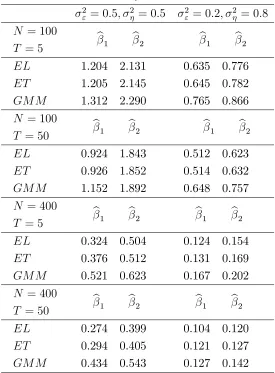
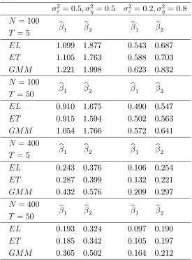
and optimal instruments are estimated using the Epanechnikov kernel with bandwidth chosen by least squares cross-validation. Tables 1 and 2 report the mean square error (MSE) of the two

estimators bβ_j( )for two combinations of the variances σ2

ε and σ2η, sample sizesN, T using both

the observed instruments zit and the optimal (estimated) instruments

b

zit = h

b

E(yit−1|uit−1),Eb(yit−1|uit−2),Eb(yit−1|uit−1, uit−2), xit i′

,

respectively. The results are based on 5000 replications, which implies that the Monte Carlo standard error is approximately 0.003.

Tables 1 and 2 approx here

The results of Tables 1 and 2 suggest that both the NPEL and the NPET estimators perform better than the 2NPGMM estimator. As expected, the estimators based on the optimal instru-ments are characterized by a smaller MSE than those based on the observed instruinstru-ments. Note also that increasing the time dimension results in estimators with a slightly lower MSE. Between the NPEL and the NPET estimator, the former seems to have an edge over the latter, which is consistent with the theoretical …ndings of Bravo (2014).

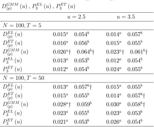
The …nite sample properties of the test statistics of Section 3.3 are investigated considering

only the case of optimal instruments with the null hypothesis speci…ed as

H0 :β10(u) =β10 = 0.3,

versus a sequence of alternatives indexed byδ = [0.0.2,0.4,0.6,0.8,1]

H1 =β10+δ(β10(u)−β10).

Table 3 reports the …nite sample size (corresponding to δ = 0) at a 0.01 and 0.05 nominal

level for the NPELDEL

Pearson type statistics PEL

3 ( )and P3ET ( )4 obtained, respectively, as a by-product of the local

empirical likelihood and exponential tilting estimation used to compute DEL

(p) ( ) and D(ETp) ( ).

The test statistics are computed at the points u = 2.5 and u = 3.5 and for two sample sizes:

N = 100, T = 5 and N = 100, T = 50, using 5000 replications and bandwidth …xed ath=have_,

where have _{is the average of the 5000 bandwidths used to obtain Table 2.}

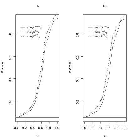
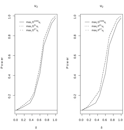
Figures 1- 4 show the size adjusted power (δ= [0.2,0.4,0.6,0.8,1]) for the …ve test statistics

considered in Table 3 obtained using 1000 replications for each value of δ.

Figures 1-4 approx here

Table 3 and Figures 1-4 illustrate that the NPIT statistics perform well and are superior to the 2NPGMM statistic both in terms of size and power. NPEL and NPET have similar …nite sample properties with the exponential tilting having a slight overall edge in terms of power. Interestingly the local Pearson’s goodness of …t type of statistics seem to be characterized by slightly better …nite sample properties than those based on the local distance statistics. In particular Table 3 suggests that the Pearson’s goodness of …t statistics are the only one with a statistically insigni…cant (at the 0.05 level) size distortion. It also suggests that the 2NPGMM statistics is always characterized by a statistically signi…cant size distortion.

Table 4 and Figure 5-6 report, respectively, the …nite sample size and power of the statistics

maxjDEL_(p) ( ), maxjD₍ET_p) ( ), maxjD₍GM M_p) ( ), maxjP3EL( ), maxjP3ET ( ) evaluated at {uj}10_j=1

where uj = 2 + 0.15j.

Figures 5-6 approx here

Table 4 and Figures 5-6 con…rm the …ndings of Table 3 and Figures 1-4 as they suggest that the tests based on NPEL and NPET have better …nite sample properties than those based on 2NPGMM with the exponential tilting having an edge over the empirical likelihood. Note that in this case also the NPEL and NPET statistics have a statistically signi…cant size distortion.

Overall the results of the simulations are encouraging and suggest that the NPIT approach can be a valid alternative to the 2NPGMM approach that has been used for smooth coe¢cients dynamic panel data models. NPIT estimators seem to be characterized by a smaller MSE while NPIT test statistics are typically less size distorted and more powerful than those based on 2NPGMM.

5

Supplemental appendix

Throughout the Appendix “CMT”, “CLT” and "LLN" denote Continuous Mapping Theorem,

Central Limit Theorem, and Law of Large Numbers, respectively. C denotes an arbitrary

4_{The results for the statisticsP}EL

positive constant that may di¤er from line to line, n =N T and …nally unless otherwise stated P

=:PN_i=1PT_t=1.

Proof of Theorem1. Suppose that for a givenu,βe(u)→p β₀(u); let_eεit =yit−x′iteβ(u), and note that

eεit =εit+x′it βe(u)−β0(u) . (19)

The same arguments of Cai and Li (2008, Proposition 2(i)) show that

hp

n

X

z⊗2

it εitx′it βe(u)−β0(u) Kh(uit−u)2 = op(1),

hp

n

X

zitx′it βe(u)−β0(u) Kh(uit−u)

⊗2

≤

e

β(u)−β₀(u) 2 h p

n

X

(zitx′itKh(uit−u))⊗2 = op(1)Op(1),

hp

n

X

(zitεitKh(uit−u))⊗2−f(u) 0(u)ν0 = op(1),

hence

hp

n

X

(ziteεitKh(uit−u))⊗2−

hp

n

X

(zitεitKh(uit−u))⊗2 =op(1), (20) and therefore by the triangle inequality

hp

n

X

(ziteεitKh(uit−u))⊗2−f(u) 0(u)ν0 =op(1). (21)

By a second order Taylor expansion about λ= 0 and (21)we have that

0 ≤ 1

nΓ

CR _{eβ, λ, u −} 1

nΓ

CR _{β,e 0, u =−λ(u)}′ 1

n

X

ziteεitKh(uit−u)− 1

2λ(u)

′ 1

n

X

(ziteεitKh(uit−u))⊗2λ(u) = −λ(u)′ 1

n

X

ziteεitKh(uit−u)− 1 2hpλ(u)

′

(z)f(u)ν0λ(u) +op(1),

so that by the quadratic approximation lemma (Fan and Gijbels 1996) the maximizer bλ(u) of

ΓCR e_{β, λ, u is given by}

b

λ(u) =−( 0(u)f(u)ν0)−1

hp

n

X

ziteεitKh(uit−u) +op(1). (22)

Using (19) the triangle inequality and the CLT applied to PzitεitKh(uit−u)/n (see Cai and

Li (2008, Theorem 2)) imply that

b

λ(u) ≤C h

p

n

X

zitεitKh(uit−u) +op(1) =Op

n hp

−1/2

Letθn =−(n/hp)−1/2ρθ, wherekθk= 1 and ρ=Op(1); note that max

i,t kzitεitKh(uit−u)k ≤

X 1

hp kzitεitK(uit−u)k (24)

≤ n1/2(1+δ) 1

nhp X

kzitεitK(uit−u)k2(1+δ)

1/2(1+δ)

= Op n1/2(1+δ)

by Jensen’s inequality and a standard kernel calculation that shows that 1

nhp X

kzitεitK(uit−u)k2(1+δ) =Op(1).

Similarly maxi,tkzitx′itKh(uit−u)k=Op n1/2(1+δ) , hence

max i,t |θ

′

nziteεitKh(uit−u)| ≤max i,t |θ

′

nzitεitKh(uit−u)|+ (25) e

β(u)−β₀(u) max i,t kθ

′

nzitx′itKh(uit−u)k=op(1).

Note also that by (19), (20) and A3, for any unit vector θ

σmax

hp

n

X

(zitεitKh(uit−u))⊗2 +op(1) ≥θ′

hp

n

X

(ziteεitKh(uit−u))⊗2θ (26)

≥ σmin

hp

n

X

(zitεitKh(uit−u))⊗2 +op(1)>0 +op(1),

whereσmax( )andσmin( )denote, respectively, largest and smallest eigenvalues andeεitis de…ned

in(19).

Let bβ(u)denote the local minimizer of ΓECR_{(β, λ, u),}

bεit =yit−x′itβb(u)

denote the resulting residual and assume that bβ(u)−β₀(u) = op(1). Using (26) and as in

the proof of Lemma A3 of Newey and Smith (2004), a Taylor expansion about θn = 0 shows

that 1

nΓ

CR _{β, θb}

n, u = 1

nΓ

CR _{bβ,0, u −θ}′

n 1

n

X

(zitbεitKh(uit−u))− (27) 1 2θ ′ n 1 n X

(zitbεitKh(uit−u))⊗2θn

≥ 1

nΓ

CR _{bβ,0, u −} hp

n

1/2

ρ 1 n

X

(zitbεitKh(uit−u)) −Cρ2 1

n ,

which implies

1

nΓ

CR _{bβ,0, u +ρ} hp

n

1/2

1

n

X

(zitbεitKh(uit−u)) −Op 1

n ≤

1

nΓ

CR _{bβ, θ}

n, u ≤ 1

nΓ

CR _{β,b bλ, u ≤} 1

nΓ

CR_(β

0,0, u) +Op

hp

Rearranging (27) it follows that

ρ 1 n

X

(zitbεitKh(uit−u)) ≤op

hp

n

1/2!

+Op

1

nhp

1/2!

→0,

which, given (19) with bβ( )replacing βe( ), implies

1

n

X

(zix′itKh(uit−u)) βb(u)−β0(u) =op(1).

By the rank condition A2(i) it then follows that bβ(u)−β0(u) = op(1). The asymptotic

distribution ofβb( )is obtained by a standard mean value expansion. By the consistency ofbλ( )

and bβ( )the …rst order conditions 0 =∂ΓECR β,b bλ, u /∂(λ′, β′)′ are satis…ed with probability

approaching 1, hence expanding about 0and β0( )we have

0 = −

"

1

n P

(zitεitKh(uit−u)) +bn(u) 0 # + 1 n  

P∂2_ΓCR_(β,λ,u)

∂λ⊗2

P∂2_ΓCR_(β,λ,u)

∂λ∂β′ P∂2_ΓCR_(β,λ,u)

∂β∂λ′

P∂2_ΓCR_(β,λ,u)

∂β⊗2

 

"

b

λ(u) b

β(u)−β0(u)

#

,

where

bn(u) = 1

n

X

xitzit′ (β(uit)−β0(u))Kh(uit−u), (28)

andβ =:β(u), λ=:λ(u)are the mean values. By(25)withθn=λ,maxit λ

′

zitεitKh(uit−u) =

op(1), whereεit=yit−x′itβ(u)is the mean value residual, hence as in Newey and Smith (2004)

max

i,t 1 +γλ(u)

′

zitεitKh(uit−u)

1

γ−j

−1 = op(1) forj = 0,1; (29)

the triangle inequality and(29)show that

1

n

X∂2_ΓCR _{β, λ, u}

∂λ⊗2 ≤ maxi,t 1 +γλ(u)

′

zitεitKh(uit−u)

1

γ−1

−1 ×

−1

n

X

(zitεitKh(uit−u))⊗2 +

−1

n

X

(zitεitKh(uit−u))⊗2

= −1

n

X

(zitεitKh(uit−u))⊗2 +op(1),

hence by (21)

hp

n

X∂2_ΓCR _{β, λ, u}

Similarly

1

n

X∂2ΓCR β, λ, u

∂λ∂β′ ≤ maxi,t 1 +γλ(u)

′

zitεitKh(uit−u)

1

γ−1

−1 ×

1

n

X

λ′zitεitzitxit′ Kh(uit−u)2 + 1

n

X

λ′zitεitzitxit′ Kh(uit−u)2 +

max

i,t 1 +γλ(u)

′

zitεitKh(uit−u)

1

γ _{−1 ×}

1

n

X

(zitx′itKh(uit−u)) + 1

n

X

(zitx′itKh(uit−u)) ,

and by the Cauchy-Schwarz inequality and the same arguments used to establish (19) and (21)

it follows that

λ n

X

zitεitzitx′itKh(uit−u)2 ≤ λ 1

n

X

kzitεitKh(uit−u)k2

1/2

1

n

X

kzitx′itKh(uit−u)k2

1/2

= op(1)Op(1),

1

n

X

(zitx′itKh(uit−u))−f(u) Σ0(u) =op(1), hence

1

n

X∂2_ΓECR _{β, λ, u}

∂λ∂β′ −f(u) Σ0(u) = op(1). (31)

Finally similar arguments can be used to show that

X∂2_ΓCR _{β, λ, u}

∂β⊗2 =op(1). (32)

Combining(30)-(32)and the CMT imply

(nhp)1/2 "

b

λ(u)/hp b

β(u)−β₀(u) #

= "

−f(u) 0(u)ν0 Σ0(u)

Σ0(u)′ 0

#−1

× (33)

(nhp)1/2 "

1

n P

(zitεitKh(uit−u)) +bn(u) 0

#

By a standard kernel calculation

E(bn(u)) = Z

xitz′it "

∂β₀(u)

∂u′ (uit−u) +

1 2

p X

j=1

∂2_β 0(u)

∂u′_∂u

j

(uit−u) (uit−u)_j #

×

Kh(uit−u)f(zit, xit, uit)dzitdxitduit =

h2

2 E xitz

′

it tr f(u) 2

∂2_β 0(u)

∂u′_∂u

j

+ 2 ∂f(zit, xit, uit)

f(zit, xit|uit =u)∂uj

∂β₀(u)

∂u′ |uit=u]

+O h3 .

The asymptotic normality of (hp₎1/2P

(zitεitKh(uit−u))/n1/2 can be established using

Lya-punov CLT, since A6 can be used to verify the LyaLya-punov condition - see also Cai and Li (2008, Theorem 2), and the result follows by the CMT.

Proof of Theorem 2. The proof of the theorem is the same as that of Theorem 1 with the

exception of the CLT used. The …rst result (i.e. the small N large T) is obtained following

closely Cai (2003). For a unit vector θ let(vit)T_t=1 =

n (hp₎1/2

θ′zitεitKh(uit−u) oT

t=1, which for

each i is a stationary α-mixing sequence. Using Proposition 2(ii) of Cai and Li (2008) it is

possible to show that V ar PT_t=1vit/T1/2 =θ′f(u) 0(u)ν0θ, hence by the i.i.d. assumption

V ar 1

(N T)1/2 N X i=1 T X t=1 vit !

=θ′f(u) 0(u)ν0θ :=σ2(u). (34)

To show the asymptotic normality the indices 1, ..., T are partitioned using Doob’s small-block

large block technique into 2qT + 1 subsets with the large block of size r =: rT = ⌊(nhp)1/2⌋

and the small one of size s =:sT = ⌊(nhp)1/2/logT⌋, q =: qT = ⌊T /(r+s)⌋ where ⌊ ⌋ is the

integer part function and note that s/r → 0, r/T → 0 and (T /r)α(s)→ 0. For0 ≤j ≤ q let

Vij,1 =Pj_t=(r_j+_(rs₊)+_s)+1r vit, Vij,2 =P_t(₌j+1)(_j(r+r_s+₎₊s)_r+1vit,Viq =PTt=q(r+s)+1vit so that

1

n1/2

X

vit= 1

n1/2

N X

i=1

q−1

X

j=0

(Vij,1+Vij,2) +Viq !

=: Un1+Un2+Un3

n1/2 .

The same arguments used by Cai (2003) show thatE(U2

n2/n) =

PN i=1V ar

Pq−1

j=0Vij,2/T1/2 /N =

o(1) and E(U2

n3/n) =

PN

i=1V ar Viq/T1/2 /N = o(1), hence Un2 = op n1/2 and Un3 =

op n1/2 . Furthermore for any 1≤i≤N and ι= (−1)1/2

Eexp ιt

q−1

X

j=0

Vij,1

!

−

q−1

Y

j=0

Eexp (ιtVij,1) ≤16α(T /r)α(s)→0 (35)

by Lemma 1.1 of Volkonskii and Rozanov (1959). Note that by A1’

1

N T

N X

i=1

q−1

X

j=0

E(Vij,1)2 =

qr T

1

rV ar

r X

t=1

vit !

whereσ2_{(u)is de…ned in(34). Finally as shown by Cai (2003)E V}2

i1,1I |Vi1,1| ≥ǫσ(u)T1/2 =

O T−δ/2_r2(2+δ)_h−p(2+δ)δ/2(1+δ) _{for every ǫ >0, hence}

1

N T

N X

i=1

q−1

X

j=0

E V_ij,2₁I |Vi1,1| ≥ǫσ(u)T1/2 =O Tδ/4h−p[1+2/(1+δ)]δ/4 →0 (37)

by A7. Thus(35)−(37) imply the Lindeberg-Feller CLT and the result follows by CMT.

For the large N and large T case consider the doubly indexed sequence

{vit}ni,t=1 =

n

(hp)1/2θ′zitεitKh(uit−u) on

i,t=1,

which is independent across i and stationary α−mixing across t, and note that both (35) and

(36) are still valid for N, T → ∞. The joint asymptotic normality as N, T → ∞ is

estab-lished applying Theorem 2 of Phillips and Moon (1999) and verifying the generalized Lindeberg condition

1

σ2

N(u) N X

i=1

E V_ij,2₁I(|Vi1,1| ≥ǫσN(u)) →0, (38)

where σ2

N(u) = V ar PN

i=1

Pq−1

j=0Vij,1/T1/2 . By(36) σ2N(u) =O(N)and

sup

1≤i≤N

E

q−1

X

j=1

V_ij,2₁/T1/2

!

<∞,

hence Theorem 23.10 of Davidson (1994) implies that(38)holds. Thus by Theorem 2 of Phillips

and Moon (1999)Pvit/n1/2

d

→N(0, σ2_{(u)) and the result follows by CMT.}

Proof of Theorem 3. For the parametric case _bzit =g(wit,bγ) note that

hp

n

X

(z_bitεitKh(uit−u))⊗2 =

hp

n

X

(zitεitKh(uit−u))⊗2+ (39) 2h

p

n

X

(z_bit−zit)zit′ (εitKh(uit−u))2 +

hp

n

X

(_bzit−zit) (Kh(uit−u))⊗2 . As in Owen (1990), A8(i) and an application of the Borel-Cantelli lemma gives

max i,t sup_γ∈Γ

∂g(wit, γ)

∂γ′ =op n

1/2 _,

hence a mean value expansion and A8(i) show that

max

i,t kzbit−zitk ≤maxit

∂g(wit, γ)

where γ is the mean value, hence using(40)in (39) yields

hp

n

X

(_bzit−zit)zit′ (εitKh(uit−u))2 ≤max

i,t kzbit−zitk ×

hp

n

X

zit(εitKh(uit−u))2 =op(1),

hp

n

X

((z_bit−zit)εitKh(uit−u))⊗2 ≤max

i,t kzbit−zitk

2

×

hp

n

X

(εitKh(uit−u))2 =op(1),

hence

hp

n

X

(_bzitεitKh(uit−u))⊗2 =

hp

n

X

(zitεitKh(uit−u))⊗2+op(1) ; therefore by triangle inequality

hp

n

X

(_bzitεitKh(uit−u))⊗2−f(u) 0(u)ν0 =op(1). (41)

Let_eεit = yit−x′iteβ(u) for any consistent estimator eβ(u); by triangle inequality and similarly

to(24)

max i,t |θ

′

nzbiteεitKh(uit−u)| ≤max

i,t kbzit−zitkmaxi,t |θ

′

neεitKh(uit−u)|+ (42) max

i,t |θ

′

nziteεitKh(uit−u)| ≤max

i,t kbzit−zitk kθnkmaxi,t |εitKh(uit−u)|+ e

β(u)−β₀(u) max

i,t kzbit−zitk kλnkmaxi,t kxitKh(uit−u)k=op(1).

Using the same Taylor expansion argument as that of Theorem1it can be shows that the 2NPIT

estimator βb(u) is consistent. To establish the asymptotic normality note that

1

n

X

(_bzitbεitKh(uit−u)) = 1

n

X

(_bzit−zit)εitKh(uit−u) + (43) 1

n

X

zitεitKh(uit−u) + 1

n

X

(z_bit−zit)x′it βb(uit)−β0(u) Kh(uit−u) +bn(u),

where bn(u) is de…ned in (28). Since

(nhp)1/2 1

n

X

(_bzit−zit)εitKh(uit−u) ≤ (44)

max

i,t kbzit−zitk(nh

p₎1/2 1

n

X

εitKh(uit−u) =op(1)Op(1),

and similarly for

1

n

X

the conclusion follows by the same arguments as those used in Theorems 1 or 2. For the

nonparametric case note …rst that by Masry (1996) sup_i,tkz_bit−zitk = op(1) hence as in (41)

and (42)

hp

n

X

(z_bitεitKh(uit−u))⊗2−f(u) 0(u)ν0 = op(1), (45) max

i,t |λ

′

nbziteεitKh(uit−u)| = op(1),

and the consistency of the 2NPIT estimator follows as before. By a standard kernel calculation

(_bzit−zit) = X

j6=i,t

Wnb(wjt−wit)vjt +op(1), (46)

where Wnb(wjt−wit) =Wb(wjt−wit)/[(n−1)f(wit)]; note that by A1 (or A1’) if i 6=i′ and

j 6=j′ _{the terms involved in the following summation}

nhpV ar 1 n

X

i,t X

j6=i

Wnb(wjt−wit)vjtεitKh(uit−u) !

= (47)

hp

nCov

X

i,t X

j6=i

Wnb(wjt−wit)vjtεitKh(uit−u)

X

i′_,t′ X

j′_6=i′

Wnb(wj′_t′ −w_i′_t′)v_j′_t′ε_i′_t′K_h(u_i′_t′−u) !

,

are 0, hence it su¢ces to consider only the two cases i =i′ _{and j =j}′_{. ForT …nite and t =t}′

by conditioning …rst onwit and then on uit and a standard kernel calculation show that

hp

n

X

i,t X

j6=i X

j′_6=i

Cov(Wb(wjt−wit)vjtεitKh(uit−u), Wb(wj′_t−w_it)v_j′_tε_itK_h(u_it−u)) ≤

b2kf(u)E(V ar(vitεit|wit)|uit =u)v0k+

hpb2Tkf(u)E[Cov(vitεit, visεis|wit, wis)|uit=u]v0k=O b2

and similarly for t 6= t′_{; for the case j = j}′ _{and t = t}′ _{noting that for (u}

it−u)/b = v by A5’

(ui′_t−u)/h=v+o(1) it follows that

hp

n

X

i,t′_,t X

j6=i X

j6=i′

Cov(Wb(wjt−wit)vjtεitKh(uit−u), Wb(wjt−wi′_t)v_j′_tε_itK_h(u_i′_t−u)) ≤

b2

Z

V ar(vitεit|w1it=w1, uit=u)w0dwitv0 +

hpb2T

Z

where w0 =

R

W(v)2dv.

For T → ∞ and i=i′_{, t=t}′ _{the Cauchy-Schwarz inequality applied to(47) shows that}

h n

p_X

i,t X

j6=i X

j′_6=i

Cov(Wb(wjt−wit)vjtεitKh(uit−u), Wb(wj′_t−w_it)v_j′_tε_itK_h(u_it−u))

2

≤

X

t

α(t)f(w)|v0E[V ar(εit|wit)|wit=w]|1/2×

kV ar(vjtE[Wb(wjt−wit)Wb(wj′_t−w_it)|w_it])k ≤Cb2 X

t

α(t) =O b2

and similarly for t6=t′_{. For the case j =j}′ _{and t=t}′

hp

n

X

i,t′_,t X

j6=i X

j6=i′

Cov(Wb(wjt−wit)vjtεitKh(uit−u), Wb(wjt−wi′_t)v_j′_tε_itK_h(u_i′_t−u))

2

≤

b2 1 n(n−1)

X

i,j,t X

j6=i

α(t) Z

v0V ar(vjtεit|wit)w0dwit ×

1

n(n−1) X

i,i′_,t X

j6=i X

j6=i′

α(t) Z

V ar(vjtεit|Wb(wjt−wit)Wb(wjt−wi′_t))w₀dw_jt

and similarly for t6=t′_{. Hence it follows that}

nhpV ar 1 n

X

i,t X

j6=i

Wnb(wjt−wit)vjtεitKh(uit−u) !

=o(1)

and

1

n

X

(_bzit−zit)εitKh(uit−u) =op (nhp)−1/2 . (48) Using similar arguments it is possible to show that

nhpV ar 1 n

X

i,t X

j6=i

Wnb(wjt−wit)vjtx′it(β(uit)−β0(u))Kh(uit−u) !

=op(1),

hence

hp

n

1/2_X

(_bzitbεitKh(uit−u)) = 1

n

X

zitεitKh(uit−u) +bbn(u) +op(1),

and the result follows again by the same arguments as those used in the proofs of Theorems 1

or2.

reminder λ=:λ(u) - that isλ is on the line joining 0and bλ- it follows that

ΓCR bβ,bλ, u −ΓCR bβ,0, u =−bλ(u)′XzitbεitKh(uit−u) +

1 2bλ(u)

′ 1

n

X∂2_ΓCR b_{β, λ, u}

∂λ⊗2 λb(u)

= h

p

n

X

(zitbεitKh(uit−u))′(f(u) (u)ν0)−1

X

(zitbεitKh(uit−u)) +op(1),

where the second equality follows using (21) (with_bεit replacingeεit) and(22). Since

X

(zitbεitKh(uit−u)) = X

(zitεitKh(uit−u))− X

(zitx′itKh(uit−u))

Σ0(u)′ 0(u)−1Σ0(u)

−1

Σ0(u)′ 0(u)−1

X

(zitεitKh(uit−u)) +op

hp

n

1/2!

,

it follows that

DCR(u) = h p

n

X

(zitεitKh(uit−u))′(f(u) (u)ν0)−1/2M0(u)× (49)

(f(u) (u)ν0)−1/2

X

(zitεitKh(uit−u)) +op(1),

where

M0(u) = I−(f(u) (u)ν0)−1/2Σ0(u) (Ξ0(u)f(u)/ν0)−1

Σ0(u)′(f(u) (u)ν0)−1/2,

and the conclusion follows by a standard result on the distribution of quadratic forms in normal vectors with idempotent matrices, see e.g. Theorem 7.2 of Rao (1973). For the case of the

estimated instrumentsz_bit using (41), (42) or(45)it follows that

ΓCR β,b bλ, u −ΓCR bβ,0, u =−bλ(u)′X_bzitbεitKh(uit−u) + (50) 1

2bλ(u)

′X

(_bzitεitKh(uit−u))⊗2bλ(u)

= h

p

n

X

(zitbεitKh(uit−u))′(f(u) (u)ν0)−1

X

(zitbεitKh(uit−u)) +

Op(1)

hp

n

1/2_X

(z_bit−zit)bεitKh(uit−u) +

1 2bλ(u)

′ hp

n

X

((z_bit−zit)bεitKh(uit−u))⊗2bλ(u)

= h

p

n

X

(zitbεitKh(uit−u))′(f(u) (u)ν0)−1

X

(zitbεitKh(uit−u)) +op(1)

Proof of Theorem 5. By a mean value expansion about λ = 0

∂π_bCR_it bβ,bλ, u

∂λ =

1

n −

1

n 1 +γλ(u)

′

zitbεitKh(uit−u)

1

γ−1 b

λ(u)′(zitbεitKh(uit−u))

where λ=:λ(u)is the mean value. By (25) and (29) it follows that

∂_bπCR_it bβ,λ, ub

∂λ =

1

n −

1

nbλ(u)

′

(zitbεitKh(uit−u)) +op 1

n , (51)

hence nπ_bit β,b λ, ub −1 =bλ(u)′(zitbεitKh(uit−u)) +op(1) and thus

X

n_bπCRit bβ,λ, ub −1

2

=bλ(u)′X(zitbεitKh(uit−u))⊗2bλ(u) +op(1) = (52)

hp

n

X

(zitbεitKh(uit−u))′(f(u) (u)ν0)−1

X

(zitbεitKh(uit−u)) +op(1),

so that the result follows as in the proof of Theorem 4. The second result follows noting that

X nπ_bCR_it β,b bλ, u −1 2

nπ_bCR_it bβ,bλ, u =

X

n_bπCR_it β,b λ, ub −1 2(1 +op(1)) (53)

as maxi,t λb(u)′(zitbεitKh(uit−u)) = op(1). For the case of estimated instrumentszbit,

∂_bπCR_it bβ,λ, ub

∂λ =

1

n −

1

nbλ(u)

′

(_bzitbεitKh(uit−u)) +op 1

n ,

and by (50)

X

n_bπCR_it β,b bλ, u −1 2 = h p

n

X

(z_bitbεitKh(uit−u))′(f(u) (u)ν0)−1

X

(_bzitbεitKh(uit−u)) +op(1)

= h

p

n

X

(zitbεitKh(uit−u))′(f(u) (u)ν0)−1

X

(zitbεitKh(uit−u)) +op(1)

and the conclusion follows by the same arguments as those used in the proof of Theorem4.The

conclusion for P n_bπCR_it β,b bλ, u −1 2/n_bπCR_it β,b bλ, u follows by (52) and (53).

Proof of Corollary 5.1. Under the local Pitman alternative and (nhp₎1/2

1 and 2 imply that P(zitεitKh(uit−u))/(nhp)1/2 d

→ N(γ(u)f(u), 0(u)v0f(u)), hence

as in (49) the result for DCR_{(u) follows by standard results on the distribution of quadratic}

forms in nonzero mean normal vectors with idempotent matrices, see e.g. Theorem 7.2 of Rao

(1973). The consistency under the condition(nhp₎1/2

γ_n(u)→ ∞is a direct consequence of the

previous conclusion. The result for PCR

j (u) (j = 1,2) follows by (52) and (53), which imply

that PCR

j (u) =DCR(u) +op(1).

Proof of Theorem 6. It is …rst shown that for any two distinct uj and uk for 1≤j, k ≤m

hp

nCov

X

(zitεitKh(uit−uj)), X

(zisεisKh(uis−uk)) =o(1). (54)

ForT …nite, iterated expectations and a standard kernel calculation show that

Cov(zitεitKh(uit−uj),(zisεisKh(uis−uk))) = 1t(ui1, uis)f(uj, uk), hence by A1

hp

nCov

X

(zitεitKh(uit−uj)), X

(zisεisKh(uis−uk)) = hpT O(1) (55)

→ 0.

ForT → ∞ letdn be an integer such that dnhp →0; then by

hpX (zitεitKh(uit−uj)), X

(zisεisKh(uis−uk)) = (56)

hp dn X

s=1

kCov(zitεitKh(uit−uj), zisεisKh(uis−uk))k+

hp

T X

s=dn+1

kCov(zitεitKh(uit−uj), zisεisKh(uis−uk))k ≤dnhp+ h−p

γ

2+γ Xα(s) γ

2+γ →0

by(55),EkzitεitKh(uit−uj)k2+γ =O h−p(1+γ) , A7 and an application of Davidov’s inequality

(Hall and Heyde 1980, p. 278) that shows that

kCov((zi1εi1Kh(ui1−uj), zisεisKh(uis−uk)))k ≤ Cα(s)

γ

2+γ E kz

i1εi1Kh(ui1−uj)k2+γ

1 2+γ

E kzisεisKh(uis−uj)k2+γ

1 2+γ

.

Thus by(54), the same CLTs used in the proofs of Theorems1 and 2can be used to show that

hp

n

1/2

  

P

(zitbεitKh(uit−u1))

... P

(zitbεitKh(uit−um))  

→d (57)

N 0, diag[f(u1) 0(u1)ν0−P0(u1), ..., f(um) 0(um)ν0 −P (um)]

!

where diag[ ] indicates a diagonal matrix and

P0(u) = Σ0(u) (Ξ0(u)f(u)/ν0)−1Σ0(u)′. (58)

The result for maxjDCR(uj)follows by (49),(57)and the CMT, which imply that

max j

hp

n

X

(zitbεitKh(uit−uj))′(f(uj) (uj)ν0)−1

X

(zitbεitKh(uit−uj)) d

→

max j χ

2

j(l−k).

The result formaxjPkCR(uj) (k = 1,2)follows similarly using (52) and (53). For the estimated

instrumentsz_bit we have

Cov(z_bitεitKh(uit−uj),bzisεisKh(uis−uk)) =

Cov((z_bit−zit)εitKh(uit−uj),(bzis−zis)εisKh(uis−uk)) + 2Cov((z_bit−zit)εitKh(uit−uj),bzisεisKh(uis−uk)) +

Cov(zitεitKh(uit−uj), zisεisKh(uis−uk)),

and for the parametric case

kCov(_bzitεisKh(uit−uj),zbisεisKh(uis−uk))k= b

β−β₀ 2 ∂g_1t (ui1, uis)f(uj, uk) =op(1),

and similarly for the second term, whereas for the nonparametric case, (46) and a standard

kernel calculation shows that

kCov(z_bitεitKh(uit−uj),bzisεisKh(uis−uk))k=

k 1t(ui1, uis)f(uj, uk)k+O b2 ,

and similarly for the second term; thus by either(55)or (56)

hp

nCov

X

(z_bitεitKh(uit−uj)), X

(_bzisεisKh(uis−uk)) →0,

and the result follows using (49), (52), (53), (57) and the CMT.

Proof of Corollary 6.1. The same arguments as those used in the proof of Corollary5.1and

Theorem6 show that under the local Pitman alternative and (nhp₎1/2_γ

n(uj)→ γ(uj) >0 for

j = 1, ..., m

X

(zitεitKh(uit−uj))/(nhp)1/2 d

→N(γ(uj)f(uj), 0(uj)v0f(uj))

and for any two distinct uj and uk for 1≤j, k ≤m

hp

nCov

X

[(zitεit−γn(uj))Kh(uit−uj)], X