DynamicWEB: A Conceptual Clustering
Algorithm for a Changing World
Joel David Scanlan, BComp. (Hons)
A dissertation submitted to the Faculty of Science, Engineering
and Technology, University of Tasmania in fulfilment of the
requirements for the Degree of Doctor of Philosophy.
Statement of Originality
I
S
TATEMENT OF
O
RIGINALITY
This thesis contains no material which has been accepted for a degree or diploma by the University or any other institution, except by way of background information and duly acknowledged in the thesis, and to the best of my knowledge and belief no material previously published or written by another person except where due acknowledgement is made in the text of the thesis, nor does the thesis contain any material that infringes copyright.
Statement of Authority of Access
II
S
TATEMENT OF
A
UTHORITY OF
A
CCESS
This thesis may be made available for loan and limited copying in accordance with the Copyright Act 1968.
Statement of co-authorship
III
S
TATEMENT OF CO
-
AUTHORSHIP
The publications of the work undertaken in the course of this research are the following:
Scanlan, JD and Hartnett, JS and Williams, RN (2005). Identifying Reconnaissance Activity: A Strategy for Network Defence. Proceedings of 6th Australian Information Warfare & Security Conference, 24-25 November 2005, Geelong, pp. 210-215
• Mr. Joel Scanlan (80%) is the primary author. He proposed the initial research question, conducted the research and prepared the material for publication.
• Jacky Hartnett (10%) and Dr Raymond Williams (10%) of the School of Computing and Information Systems, University of Tasmania, both provided general guidance and editing advice as supervisors.
Scanlan, JD and Hartnett, JS and Williams, RN (2006) Dynamic WEB: Profile Correlation Using COBWEB. Proceedings of the 19th Australian Joint Conference on Artificial Intelligence, 4-8 December, 2006, Hobart, Tasmania, pp. 1059-1063
• Mr. Joel Scanlan (80%) is the primary author. He proposed the initial research question, conducted the research and prepared the material for publication.
• Jacky Hartnett (10%) and Dr Raymond Williams (10%) of the School of Computing and Information Systems, University of Tasmania, both provided general guidance and editing advice as supervisors.
- VIII -
• Mr. Joel Scanlan (80%) is the primary author. He proposed the initial research question, conducted the research and prepared the material for publication.
• Jacky Hartnett (10%) and Dr Raymond Williams (10%) of the School of Computing and Information Systems, University of Tasmania, both provided general guidance and editing advice as supervisors.
Scanlan, JD and Hartnett, JS and Williams, RN (2008). DynamicWEB: A method for reconnaissance activity profiling. Proceedings 2008 International Symposium on Parallel and Distributed Processing with Applications (ISPA-08), 10-12 December 2008, Sydney Australia
• Mr. Joel Scanlan (80%) is the primary author. He proposed the initial research question, conducted the research and prepared the material for publication.
• Jacky Hartnett (10%) and Dr Raymond Williams (10%) of the School of Computing and Information Systems, University of Tasmania, both provided general guidance and editing advice as supervisors.
Scanlan, JD and Hartnett, JS and Williams, RN (2008). DynamicWEB: Adapting to concept drift and object drift in COBWEB. Proceedings 21st Australasian Joint Conference on Artificial Intelligence , 1-5 December 2008, Auckland, New Zealand, pp. 454-460.
• Mr. Joel Scanlan (80%) is the primary author. He proposed the initial research question, conducted the research and prepared the material for publication.
Statement of co-authorship
Scanlan, JD and Hartnett, JS and Williams, RN (2009). Machine Learning in a changing world. Proceedings of 3rd International Workshop on Artificial Intelligence and Technology (ASISAT), 23-24 November 2009, Hobart.
• Mr. Joel Scanlan (80%) is the primary author. He proposed the initial research question, conducted the research and prepared the material for publication.
Statement of co-authorship
We the undersigned agree with the above stated proportion of work undertaken for each of the above published manuscripts contributing to this thesis.
Signed: ………..
Date: ………..
Mrs Jacky Hartnett Supervisor
School of Computing and Information Systems University of Tasmania
Signed: ………..
Date: ………..
Dr Raymond Williams Supervisor
Abstract
IV
A
BSTRACT
This research was motivated by problems in network security, where an attacker often deliberately changes their identifying information and behaviour in order to camouflage their malicious behaviour. Addressing this problem has resulted in a new adaption to the unsupervised machine learning technique COBWEB.
In machine learning and data mining the aim is to extract patterns from data in order to discover a meaning underlying the processes that are taking place. In most cases, each object is observed once, and then the patterns that have been extracted can be used to classify newly-observed objects. Conceptual clustering aims to do this in such a way that the patterns that are learned are human readable. Concept drift algorithms allow concepts to change over time, although most undertake this in a supervised manner, which presents a challenge when looking for novel classes. This research focuses on the classification of objects that change over time across multiple observations. The objects may change their own characteristics (labelled as object drift in this research) or maintain the same characteristics, but change their identifier. In addition to this, it is also possible for the concept that describes a group of objects to itself change (known as concept drift). In addition to the possible application within the security domain, the method was generalised and tested across a range of machine learning and data mining domains. In the process it was shown that the method was robust in the presence of concept drift, which occurs when a group of objects that define a given concept change their characteristics, resulting in the definition of that concept having changed over time.
The ideas of concept drift and object drift are not only relevant within the computer security field, but can be of significance in any knowledge domain. Therefore, any method presented to address this learning problem should be generalised enough to be applicable in many application areas.
- XIV -
representation of the domain. The profiles contain derived attributes, which are formed across multiple observations of each object, with the aim of retaining knowledge of how the object has changed over time. As well as preserving context over time, Dynamic Web uses multiple trees and so, transforms the learner into an ensemble classifier.
In addition to testing the method on the security and network based datasets, a number of other datasets are also examined. A new dataset (a modified version of Quinlan’s weather dataset) is presented in order to illustrate how Dynamic Web operates in the presence of object drift. The method is also tested on several well-known machine learning datasets, some of which exhibit concept drift. Along with these artificial datasets, a group of real-world datasets, including several sourced from the Australian Bureau of Statistics, were also examined, illustrating DynamicWEB’s ability to adapt to change.
Acknowledgements
V
A
CKNOWLEDGEMENTS
My supervisors, Jacky and Ray, for their continued support and advice over the years of my PhD candidature. Their assistance in undertaking the work, this thesis and the research papers that were produced, was invaluable. Without them I would not have been able to undertake this research.
I would also like to thank Mike Cameron-Jones for his advice at several points during the research and also for proof reading a sizable portion of this thesis.
I would also like to thank Dr Rob Edmondson and Kevin Manderson for allowing me access to several network based audit logs which were used in my research.
My wonderful wife Meg, without whose love and support I doubt I would ever have been able to undertake this research. Thanks also to both of our families for being a support network to both of us while we undertook our doctoral studies.
Thanks to my two office mates over the last 4 years or so: Phil and Matt. Thanks for putting up with my awesome sense of humour and for many fun times late at night.
The Cows and FGI honours/post-grad/lecturer cricket teams for the outlet away from research each week, or the LAN parties over the years. The same goes for my Virtual World crew for weekly lunches and movie nights.
VI
TABLE OF CONTENTS
1! INTRODUCTION 1!
1.1! INTRODUCTION 2!
1.2! MOTIVATION 2!
1.3! RESEARCH AIMS 3!
1.4! THESIS OUTLINE 5!
2! CLUSTERING TECHNIQUES 7!
2.1! DATA CLUSTERING 8!
2.2! PARTITIONAL CLUSTERING 9!
2.2.1! THE K-MEANS CLUSTERING ALGORITHM ... 11!
2.3! HIERARCHICAL CLUSTERING 14! 2.3.1! CLUSTERING METHODS ... 15!
2.4! CONCEPTUAL CLUSTERING 17! 2.4.1! CONJUNCTIVE CONCEPTUAL CLUSTERING ... 19!
2.4.1.1! THE REPRESENTATION SCHEME 20! 2.4.1.2! THE REPRESENTATION FUNCTION 21! 2.4.1.3! THE ALLOCATION FUNCTION 22! 2.4.1.4! THE EVALUATION CRITERION 23! 2.4.2! PROBABILISTIC CONCEPTUAL CLUSTERING ... 24!
2.4.2.1! WITT 25! 2.4.2.2! COHESION 26! 2.4.2.3! THE WITT ALGORITHM 27! 2.5! SUMMARY 28! 3! KNOWLEDGE ACQUISITION OVER TIME 30! 3.1! TIME SERIES ANALYSIS 31! 3.2! TIME SERIES CLUSTERING 31! 3.3! ONLINE LEARNING 33! 3.3.1! INCREMENTAL VS BATCH LEARNING ... 35!
3.3.1.1! DATA DRIFT 36! 3.4! ONLINE LEARNING METHODS 36! 3.5! STAGGER 37! 3.5.1! INITIALISATION ... 38!
3.5.2! PROJECTION ... 38!
3.5.3! EVALUATION ... 40!
3.5.4! REFINEMENT ... 41!
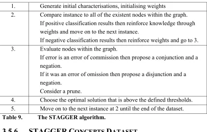
3.5.5! THE STAGGER ALGORITHM ... 43!
3.5.6! STAGGER CONCEPTS DATASET ... 43!
3.6! FLORA 45! 3.6.1! FLORA 2 ... 48!
3.6.2! FLORA3 ... 49!
3.6.3! FLORA 4 ... 50!
3.7! SUMMARY 51!
4! COBWEB 52!
4.1! INTRODUCTION TO COBWEB 53!
Table of Contents
- XVII -
4.3.1! CATEGORY UTILITY ... 58!
4.3.2! THE COBWEB ALGORITHM ... 61!
4.4! CLASSIT: EXTENDING COBWEB 63! 4.5! OTHER WORK USING COBWEB 66! 4.5.1! ARACHNE ... 68!
4.5.2! COBBIT ... 69!
4.6! SUMMARY 71! 5! DYNAMICWEB: LEARNING OVER MULTIPLE OBSERVATIONS 72! 5.1! INTRODUCTION TO DYNAMICWEB 73! 5.2! THE PROBLEM 73! 5.3! LEARNING GOALS 75! 5.4! DYNAMICWEB 77! 5.4.1! COBWEB: THE CHANGES REQUIRED ... 77!
5.4.2! SEARCH IN DYNAMICWEB ... 79!
5.4.3! UPDATE MECHANISM ... 81!
5.4.4! PROFILE ... 84!
5.4.5! MULTIPLE-DIMENSION TREE ... 87!
5.4.5.1! IMPLEMENTING DYNAMICWEB’S MULTIPLE DIMENSIONS 88! 5.5! SUMMARY 90! 6! METHOD VERIFICATION AND DEMONSTRATION 92! 6.1! INTRODUCTION 93! 6.2! VERIFYING THE COBWEB IMPLEMENTATION 93! 6.3! DYNAMIC WEATHER 97! 6.3.1! PERFORMING PROFILE UPDATES WITH DYNAMIC WEATHER ... 100!
6.3.2! TESTING THE COMPLETE DYNAMIC WEATHER DATASET ... 104!
6.3.3! PERFORMING UPDATES WITH DERIVED ATTRIBUTES ... 108!
6.4! MULTIPLE DYNAMICWEB TREES 110! 6.5! STAGGER CONCEPTS DATASET 114! 6.6! SUMMARY 120! 7! EXAMINING REAL WORLD DATASETS 121! 7.1! INTRODUCING THE DATA 122! 7.2! AUSTRALIAN NATIONAL ACCOUNTS: STATE ACCOUNTS 123! 7.3! LABOUR FORCE DATASET 130! 7.4! PHYSIOLOGICAL DATA MODELLING CONTEST 134! 7.5! SUMMARY 141! 8! PROFILING NETWORK ACTIVITY AND PERFORMANCE 143! 8.1! INTRODUCTION TO THE DATA 144! 8.2! SCAN CORRELATION 145! 8.2.1! PORT SCANS ... 145!
8.2.2! SCAN CORRELATION SYSTEMS ... 148!
8.2.2.1! THRESHOLD RANDOM WALK: SEQUENTIAL HYPOTHESIS TESTING 148! 8.2.2.2! SPADE AND SPICE: SIMULATED ANNEALING 149! 8.2.3! PREVIOUS RESEARCH ... 150!
8.3! THE PROBLEM 153!
8.4! PROFILING PORT SCANS 154!
8.6! SUMMARY 164!
9! CONCLUSIONS AND FURTHER WORK 166!
9.1! RESEARCH CONTRIBUTION 167!
9.2! RESULTS SUMMARY 169!
9.3! FUTURE DIRECTIONS 171!
10! REFERENCES 173!
11! APPENDIX A – GLOSSARY OF TERMS 179!
12! APPENDIX B – DYNAMIC WEATHER DATASET 182!
13! APPENDIX C – STAGGER CONCEPTS DATASET LISTING 185!
14! APPENDIX D – ADDITIONAL RESULTS FOR NATIONAL
ACCOUNTS DATASET 189!
15! APPENDIX E – ADDITIONAL RESULTS FOR THE LABOUR FORCE
DATASET 193!
List of Tables
- XIX -
VII
LIST OF TABLES
TABLE 1.! SIMPLE K-MEANS ALGORITHM ... 11!
TABLE 2.! CONVERGENT K-MEANS ALGORITHM ... 12!
TABLE 3.! K-MEANS WITH COARSENING AND REFINING ALGORITHM ... 13!
TABLE 4.! AGGLOMERATIVE CLUSTERING METHOD ... 15!
TABLE 5.! PAF ALGORITHM ... 21!
TABLE 6.! THE WITT ALGORITHM ... 28!
TABLE 7.! THE FOUR MAIN COMPONENTS OF STAGGER ... 37!
TABLE 8.! LISTING OF THE CHARACTERISATION WEIGHTS ... 41!
TABLE 9.! THE STAGGER ALGORITHM. ... 43!
TABLE 10.! ATTRIBUTE LISTING OF THE STAGGER CONCEPTS DATASET. ... 44!
TABLE 11.! DESCRIPTOR SETS AND THE COUNTERS ASSOCIATED WITH EACH SET .. 46!
TABLE 12.! THE LEARN FUNCTION WITHIN FLORA ... 47!
TABLE 13.! THE UNIMEM ALGORITHM ... 55!
TABLE 14.! THE EVALUATE (A) AND GENERALISE (B) FUNCTIONS USED BY THE UNIMEM ALGORITHM. ... 56!
TABLE 15.! THE COBWEB ALGORITHM ... 60!
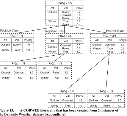
TABLE 16.! PROBABILISTIC CONCEPT DESCRIPTIONS FOR THE TWO NOMINAL ATTRIBUTES WITHIN THE WEATHER DATASET ... 62!
TABLE 17.! A COMPARISON OF PERFORMANCE A HASH TABLE AND AN AVL TREE. THE METRIC IS MEASURED IN MILLIONTHS OF A SECOND ... 79!
TABLE 18.! THE DYNAMICWEB UPDATE MECHANISM ... 81!
TABLE 19.! THE REMOVE FUNCTION OF DYNAMICWEB ... 82!
TABLE 20.! THE UPDATETREE FUNCTION OF DYNAMICWEB ... 83!
TABLE 21.! LISTING OF THE DERIVED ATTRIBUTES THAT ARE USED WITHIN THE PROFILES IN DYNAMICWEB ... 85!
TABLE 22.! THE UPDATEPROFILE FUNCTION OF DYNAMICWEB ... 86!
TABLE 23.! THE DYNAMICWEB UPDATE MECHANISM USING MULTIPLE TREES .... 89!
TABLE 24.! LISTING OF THE ATTRIBUTES WITHIN THE WEATHER DATASET ... 98!
TABLE 25.! THE CLASSES AT THE DIFFERENT POINTS OF MEASUREMENT OVER THE DAY; OBJECT DRIFTS ARE SHOWN IN BOLD. ... 98!
TABLE 26.! FIVE INSTANCES FROM THE DYNAMIC WEATHER DATASET. THE 5TH INSTANCE IS AN INSTANCE USED TO UPDATE THE 3RD INSTANCE. ... 100!
TABLE 27.! THE THREE CONCEPTS WHICH ARE PRESENT IN THE STAGGER CONCEPTS DATASET. ... 114!
TABLE 28.! A DESCRIPTION OF THE ATTRIBUTES THAT ARE WITHIN THE NATIONAL ACCOUNTS DATASET. ... 123!
TABLE 29.! INDUSTRIES THAT ARE DESCRIBED BY STATE OR TERRITORY WITHIN THE LABOUR FORCE DATASET. ... 131!
TABLE 30.! A DESCRIPTION OF THE ATTRIBUTES PRESENT IN THE PHYSIOLOGICAL DATA MODELLING CONTEST (PDMC) DATASET. ... 135!
TABLE 31.! THE THREE LOGS COVERED PERIODS OF 10, 20 AND 30 DAYS. EACH LOG RECORDED BETWEEN 11.5 AND 12 PERCENT OF SOURCE IP ADDRESSES PROBING MULTIPLE GATEWAYS WITHIN THE NETWORK. ... 151!
TABLE 33.! THE ATTRIBUTE VALUE PAIRS WITHIN THE DATASET EXAMINED.
SEVERAL ARE DERIVED AND ARE CREATED BY DYNAMICWEB.THESE ARE
UPDATED AS NEW DATA FOR THE PROFILE IS OBSERVED. ... 155!
TABLE 34.! THE ATTRIBUTES WHICH ARE PRESENT WITHIN THE ABSNETWORK
- XXII -
VIII
L
IST OF
F
IGURES
FIGURE 1.! A) A DATA SERIES. B) THE RESULTING CLUSTERS FROM A PARTITION TECHNIQUE. C) THE RESULTING TREE FROM A HIERARCHICAL TECHNIQUE. ... 8! FIGURE 2.! THE SEED POINTS ARE THE COLOURED TRIANGLES; (A) ILLUSTRATES THE
CLUSTERING THAT RESULTS FROM THE IDEAL SEED POINTS. WHILE (B) IS THE CLUSTERING THAT RESULTS FROM POORLY CHOSEN SEED POINTS. ... 10! FIGURE 3.! A) A DATA SERIES; NOW EXPRESSED WITH IDENTIFIER LABELS FOR EACH
INSTANCE. B) THE GRAPH REPRESENTATION OF THE NESTED PARTITIONS
PRODUCED BY THE HIERARCHICAL METHOD C) A DENDROGRAM DISPLAYING THE IDENTIFIERS FOR EACH INSTANCE IN THEIR RESULTING LOCATION. ... 14! FIGURE 4.! A) SINGLE LINKAGE CLUSTERING METHOD: THE CLOSEST TWO INSTANCES
WITHIN EACH CLUSTER ARE COMPARED. B) COMPLETE LINKAGE CLUSTERING METHOD: THE FURTHEST TWO INSTANCES WITHIN EACH CLUSTER ARE COMPARED.
... 16! FIGURE 5.! A ILLUSTRATION OF A CONCEPT HIERARCHY MOTOR VEHICLES ... 18! FIGURE 6.! CLUSTERING IN CONCEPTS, NOT PAIRWISE DISTANCE (MICHALSKI 1980). .
... 19! FIGURE 7.! DENDROGRAM OF THE “REALITY CHECK” DATASET (WANG, SMITH ET AL.
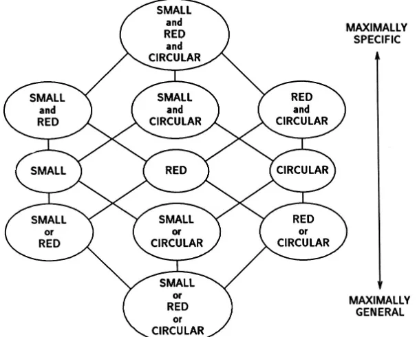
2006) ... 32! FIGURE 8.! GRAPH OF CHARACTERISATIONS PRODUCED BY STAGGER SPANNING
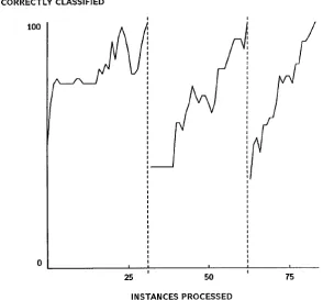
FROM MAXIMALLY SPECIFIC TO THE MAXIMALLY GENERAL (SCHLIMMER AND GRANGER 1986). ... 42! FIGURE 9.! THE LEARNING RESPONSE OF STAGGER TO CONCEPT DRIFT WITHIN THE
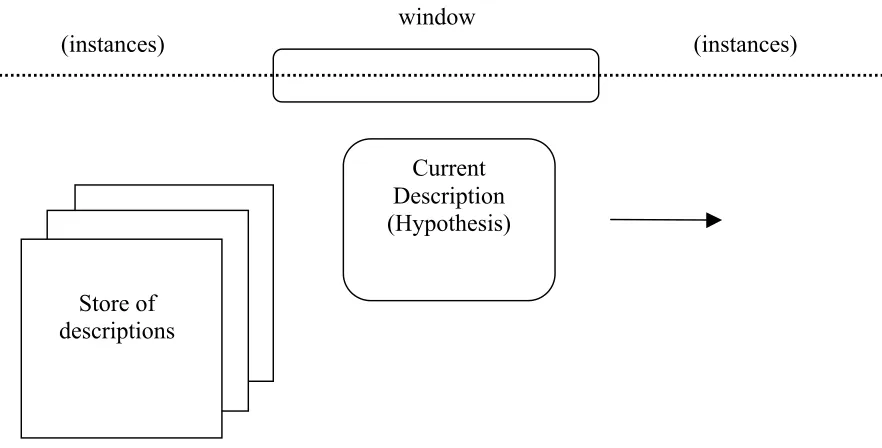
STAGGER CONCEPTS DATASET (SCHLIMMER AND GRANGER 1986). ... 44! FIGURE 10.! THE WINDOW EXAMINING A STREAM OF INSTANCES, UTILISING ONLY
THE INSTANCES WITHIN THE WINDOW TO FORM THE CURRENT HYPOTHESIS
(WIDMER AND KUBAT 1996). ... 46! FIGURE 11.! FLORA3 COMPARED TO FLORA2 AT RELEARNING THE SAME THREE
STAGGER CONCEPTS THREE TIMES (WIDMER AND KUBAT 1996). ... 49! FIGURE 12.! THE LEARNING RESPONSE TO CONCEPT DRIFT OF FLORA UPON THE
STAGGER CONCEPTS DATASET (WIDMER AND KUBAT 1996). ... 51! FIGURE 13.! A COBWEB HIERARCHY THAT HAS BEEN CREATED FROM 5 INSTANCES
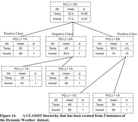
OF THE DYNAMIC WEATHER DATASET (APPENDIX A). ... 62! FIGURE 14.! A CLASSIT HIERARCHY THAT HAS BEEN CREATED FROM 5 INSTANCES
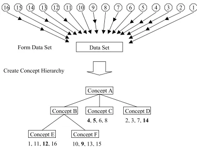
OF THE DYNAMIC WEATHER DATASET. ... 66! FIGURE 15.! THE TIME WINDOW USED WITHIN COBBIT ... 70! FIGURE 16.! IN CONCEPT DRIFT EACH OBJECT IS ONLY OBSERVED FROM ONE
INSTANCE IN THE DATASET. DURING THE CREATION OF THE HIERARCHY THE CONCEPT DESCRIPTIONS ARE ABLE TO ADAPT TO VARIATION BETWEEN INSTANCES OF THE SAME CLASS. (ARROW HEADS INDICATE THE NUMBER OF TIMES AN OBJECT HAS BEEN SAMPLED). ... 74! FIGURE 17.! OBJECT DRIFT IS THE CHANGE OF AN OBJECT ACROSS MULTIPLE
OBSERVATIONS AS RECORDED WITHIN INSTANCES IN THE DATASET. EACH OBJECT IS ABLE TO BE SAMPLED MORE THAN ONCE. ... 75! FIGURE 18.! THE AVL TREE ACTING AS AN INDEX TO THE COBWEB CONCEPT
HIERARCHY (LINKS FOR PROFILES 1 AND 7 ARE NOT SHOWN). ... 80! FIGURE 19.! THE INDEX MAPPING OUT THE LOCATION OF THE PROFILE ‘A’ WITHIN
List of Figures
FIGURE 20.! FISHER’S IMPLEMENTATION OF COBWEB VS THE DYNAMICWEB IMPLEMENTATION. ... 94! FIGURE 21.! FISHERS IMPLEMENTATION OF COBWEB VS. THE DYNAMICWEB
IMPLEMENTATION IN PREDICTING A MISSING ATTRIBUTE ... 95! FIGURE 22.! DYNAMICWEB’S IMPLEMENTATION OF COBWEB OPERATING UPON
THE QUADRUPED ANIMAL’S DATASET. ... 96! FIGURE 23.! MODIFIED C4.5 DECISION TREE OF THE WEATHER DATASET. ... 99! FIGURE 24.! THE CONCEPT HIERARCHY PRODUCED FROM THE FIRST 4 INSTANCES
SHOWN WITHIN TABLE 26. ... 101! FIGURE 25.! THE HIERARCHY WHICH OCCURS BETWEEN THE REMOVAL OF COUNTY
DOWN PROFILE AND ITS READMISSION AFTER IT HAS BEEN UPDATED. ... 102! FIGURE 26.! THE CONCEPT HIERARCHY AFTER THE 3RD
INSTANCE HAS BEEN UPDATED WITH THE NEW DATA CONTAINED WITHIN THE 5TH INSTANCE. ... 103! FIGURE 27.! THE CONCEPT HIERARCHY AFTER ONE INSTANCE OF EACH OBJECT HAS
BEEN OBSERVED. ... 104! FIGURE 28.! THE CONCEPT HIERARCHY AFTER EACH OF THE OBJECTS HAVE HAD
ANOTHER OBSERVATION AND HAVE ALL BEEN UPDATED ONCE. ... 105! FIGURE 29.! THE CONCEPT HIERARCHY AFTER THE SECOND ROUND OF UPDATES
HAVE BEEN COMPLETED. ... 106! FIGURE 30.! TRACKING THE OBJECTS OVERTIME IN RELATION TO THE OTHER
OBJECTS WITHIN THE DATASET ... 107! FIGURE 31.! THE CONCEPT HIERARCHY AFTER ALL 12 INSTANCES OF THE 4 OBJECT
SUBSET OF DYNAMIC WEATHER HAVE BEEN INCORPORATED. ... 109! FIGURE 32.! THE CYLINDER REPRESENTATIONS OF THE QUADRUPED ANIMALS
PRESENT WITHIN THE DATASET. ... 110! FIGURE 33.! PREDICTIVE ACCURACY OF THE QUADRUPED ANIMALS DATASET IN A
SINGLE CONCEPT HIERARCHY. ... 111! FIGURE 34.! THE PREDICTIVE PERFORMANCE OF THE HIERARCHIES THAT WERE EACH
FORMED ON THE DATA OF A DIFFERENT BODY PART. ... 112! FIGURE 35.! PERFORMANCE COMPARISON BETWEEN THE SINGLE COBWEB TREE
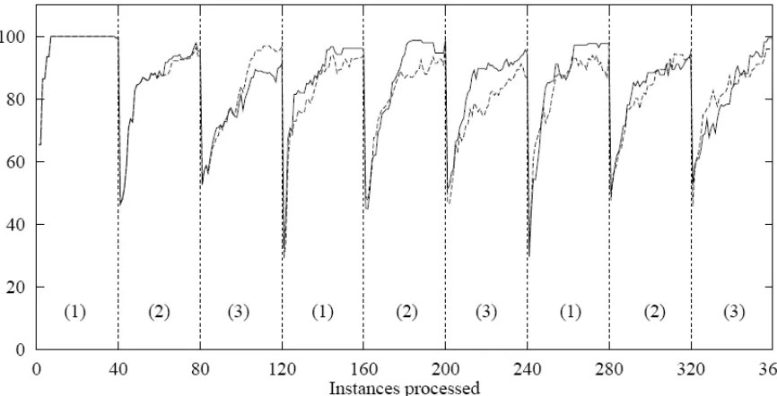
AND THE VOTED MULTIPLE TREE CONFIGURATION. ... 113! FIGURE 36.! THE LEARNING RESPONSE TO CONCEPT DRIFT OF STAGGER UPON THE
STAGGER CONCEPTS DATASET (SCHLIMMER AND GRANGER 1986). ... 115! FIGURE 37.! THE LEARNING RESPONSE TO CONCEPT DRIFT OF FLORA UPON THE
STAGGER CONCEPTS DATASET (WIDMER AND KUBAT 1996). ... 115! FIGURE 38.! THE LEARNING RESPONSE TO CONCEPT DRIFT OF DYNAMICWEB UPON
THE STAGGER CONCEPTS DATASET AVERAGED ACROSS 100 RUNS ... 116! FIGURE 39.! THE LEARNING RESPONSE OF DYNAMICWEB AND COBBIT WITH THE
TWO WINDOW SIZES OF 10 AND 20 UPON THE STAGGER CONCEPTS DATASET. 118! FIGURE 40.! THE LEARNING RESPONSE OF DYNAMICWEB AND COBBIT WITH THE
TWO WINDOW SIZES OF 40 AND 60 UPON THE STAGGER CONCEPTS DATASET. 119! FIGURE 41.! THE PERCENTAGE CHANGE AND PER CAPITA TREES WITH THE PROFILES BEING BASED ON THE FULL SET OF 17 YEARS WORTH OF DATA. ... 125! FIGURE 42.! THE PERCENTAGE CHANGE AND PER CAPITA TREES WITH THE PROFILES
BEING BASED ON A 5 YEAR WINDOW. ... 126! FIGURE 43.! THE CONCEPT DESCRIPTION OF THE TWO CHILD NODES OF THE FINAL
STRUCTURE SHOWN WITHIN FIGURE 41. ... 128! FIGURE 44.! THE CONCEPT DESCRIPTION OF THE TWO CHILD NODES OF THE FINAL
List of Figures
- XXIII -
FIGURE 45.! EIGHT STRUCTURES PRODUCED COVERING THE FOUR OBSERVATIONS THAT OCCURRED IN 1995. THE LEFT SET OF STRUCTURES REPRESENT THE FULL TIME EMPLOYEES BY INDUSTRY, AND THE RIGHT SET REPRESENT THE PART TIME EMPLOYEES. ... 132! FIGURE 46.! EIGHT STRUCTURES FORMED OVER THE YEAR 1995. THE LEFT IS
FORMED UPON THE DATA RELATING TO THE FULL TIME EMPLOYEES, WHILE THE RIGHT IS THE PART TIME EMPLOYEES USING TREND INSTEAD OF MEAN. ... 133! FIGURE 47.! LEARNING PERFORMANCE OF DYNAMICWEB UPON THE SLEEPING AND
WATCHING TV SCENARIOS USING THE MOST RECENTLY OBSERVED VALUE. ... 137! FIGURE 48.! LEARNING PERFORMANCE OF DYNAMICWEB ON THE SLEEPING AND
WATCHING TV SCENARIOS USING 2 DERIVED ATTRIBUTES TO STORE CONTEXTUAL DATA. ... 138! FIGURE 49.! COMPARISON BETWEEN THE CLASSIFICATION ACCURACIES FOR JUST
THE POSITIVE CLASS OF THE WATCHING TV SCENARIO IN THE TWO TRIALS. ... 139! FIGURE 56.! COMPARISON OF THE PREDICTIVE PERFORMANCE OF DYNAMICWEB ON
THE LAPTOP AND DESKTOP CLASSES. ... 161! FIGURE 61.! THE KNOWLEDGE HIERARCHIES PRODUCED WHEN COMPARING THE
1
Introduction
1
“Nothing in the world is permanent, and we're foolish when we ask anything to last, but surely we're still more foolish not to take delight in it while we have it. If change is of the essence of existence one would have thought it only sensible to make it the premise of our philosophy.”
William Somerset Maugham (1874 - 1965) The Razor's Edge, 1943
- 2 -
1.1
I
NTRODUCTION
The world around us is changing. In effectively every domain of knowledge, in the realms of science and industry and in people’s personal lives, change occurs in some manner, over time. Weather is monitored nightly on the news; thousands of people are employed monitoring various parts of a nation’s economy; millions world-wide earn a living from changes within the stock market; and engineers monitor infrastructure. Some change is sudden, such as the recent Global Financial Crisis, or events in our lives such as the birth of a child. Others happen more slowly, such as Climate Change or the process of aging within the human body. Observing and trying to understand change is the basis for many professions and areas of investigation.
From a computational perspective, observing and recording change, in an effort to understand it, has been carried out since the development of computers. The first stage in this process is to record data for later analysis. Machine learning is a field of computing that aims to develop methods for discovering patterns within data. Data mining is the process of applying these methods to large repositories of stored data with the aim of extracting knowledge. In the fields of machine learning and data mining, many researchers have examined datasets that contain change in various forms.
1.2
M
OTIVATION
The work reported in this thesis was inspired by a learning problem within the field of computer security. The knowledge domain is one in which many observations of a given user’s activity are recorded over a significant time period. This information, when viewed in context, presents a profile of activity that can then be used to determine whether the user is carrying out a specific type of behaviour. The security sub-field that inspired this research was related to a specific type of port scanning reconnaissance.
Chapter 1 - Introduction
activity may go from being considered benign to that of a threat (object drift). For an effective comparison to be made between these activity profiles there is a need for the context of these multiple recorded activities to be preserved.
Within the joint fields of machine learning and data mining there is an apparent lack of learning methods which observe the same objects, multiple times, over a time window. Across these observations, it is possible for the objects that are being observed to change in some way, and it is important for this change to be incorporated into the learning model.
1.3
R
ESEARCH
A
IMS
The research presented in this thesis aims to operate within the learning scenario outlined above. To enable this, the aims for the learner are as follows:
1. The learner needs to be able to profile object activity over an extended time period.
2. The learner needs to be able to establish relationships between these profiles. 3. The learner needs to be able to adapt to concept drift.
4. The learner needs to be able to adapt to object drift.
5. The leaner needs to be able to preserve context across multiple observations. 6. The learner needs to be able to track a large number of target objects
simultaneously in real-time.
These six aims outline a method that is highly adaptive with the ability to profile objects over time. The fundamental element of the learner is the production of a profile that is based on the data obtained from multiple observations of target objects over time (1). This data is a recorded history of behaviour exhibited by the target object.
- 4 -
can then be extracted from the dataset, and these patterns can then be used to model the dataset. This dataset may not have defined classes (as with the application which inspired this research), and because of this, the learner needs to be an unsupervised technique.
If the target objects1 are changing over time, then there are two forms of drift that the learner needs to be able to adjust to: concept drift and object drift (3 and 4)1. Concept drift occurs when the class description of a group of objects changes over time. For example, the definition of what is considered fashionable among a group of people may change over time as trends come and go. Object drift occurs when a target object migrates from one resultant concept to another, for example when a given person changes from being in one fashion clique of people to another.
As many observations and updates occur to the profiles relating to each target object, there is an over-arching context that needs to be preserved (5). This context is a historical one representing the past behaviour of the given object. Being able to preserve the fact that four of the numerical attributes of a particular object have been decreasing in value, over time, while a fifth attribute has been increasing in value, provides a significant benefit when it comes to classifying an object as opposed to just storing the most recent observed value of each attribute. Such preservation of contextual information is vital if behaviour is to be profiled over time.
The final aim listed above is for the learner to be able to profile a very large number of objects at once. While in many application domains the targets of interest will be few in number, the application that drove the need for this learner examines thousands of target objects simultaneously and so scalability is very important. Further, this knowledge domain, operates on live data and needs to operate in real-time to respond to any threats upon the network.
Because the machine learning method developed as part of this research will be operating in a learning environment that is quite different to that in which most methods operate it is important for it to be designed with more than just one
Chapter 1 - Introduction
application in mind. One of the main aims of this research is to produce a learning method that is generalised and applicable to a wide range of domains.
1.4
T
HESIS
O
UTLINE
The following is an overview of the chapters within this thesis
The next chapter is a brief literature review of clustering techniques within the machine-learning field, to provide some background to the way in which learning techniques extract knowledge from a dataset. This chapter will introduce the machine learning area of Conceptual Clustering.
The third chapter is an examination of clustering methods that have been developed to examine datasets in which change occurs during the learning process. These methods aim to adapt to this change and learn from it. The chapter will introduce the topic of Concept Drift, which is one of the most active areas of research within machine learning for methods that adapt to change, and the most relevant to the research described in this thesis.
The fourth chapter will describe two probabilistic conceptual clustering techniques. One of these, entitled COBWEB, has been modified in order to carry out some of the research described in this thesis. Research by other authors, also building upon this method, will be briefly examined in this chapter.
- 6 -
The seventh chapter displays DynamicWEB’s performance upon several real-world datasets, including two provided by the Australian Bureau of Statistics and one derived from a well-known data mining contest held several years ago.
The eighth chapter examines DynamicWEB’s performance on two network-based datasets. One is the scan correlation dataset that originally inspired the research and the other is a dataset detailing network performance on a network spread across the states and territories of Australia.
2
Clustering Techniques
2
“If you leave things alone you leave them as they are. But you do not. If you leave a thing alone you leave it to a torrent of
change.”
G. K. Chesterton (29 May 1874 – 14 June 1936) Orthodoxy, 1908
- 8 -
I
NTRODUCTION
In the first chapter of this thesis several goals were outlined with respect to a classification scenario involving behaviour profiling. This chapter will look at data and conceptual clustering. Data clustering is the more traditional form of clustering, and is the more frequently used technique in data mining. Conceptual clustering is however more suited to behaviour profiling, and it will be examined and contrasted with its more traditional counterpart. This is done as a precursor to the next chapter, which will examine conceptual clustering methods that adapt to change over time, and the chapters that follow, which introduce the new method being presented. This method is built upon COBWEB, an Incremental Hierarchical Conceptual Clustering Algorithm, which will be discussed in detail in Chapter 4.
2.1
D
ATA
C
LUSTERING
Clustering methods aim to discover the natural groupings of instances (items with multiple data attributes) within a given dataset. Clustering is a data mining approach in which the eventual clusters are a simplification of the data into a model. These clusters are effectively subsets within the population, with the grouping being determined by shared characteristics between instances. This model can then be utilised for classification or visualisation of the dataset. The clusters that are located are usually previously unknown, and it is through the use of these techniques that the relationships between instances (ie. patterns) are discovered.
A diverse range of clustering techniques has been developed since the late 1960s. An
Figure 1. a) A data series. b) The resulting clusters from a partition technique. c) The resulting tree from a hierarchical technique.
a b c
G F
B A C
Chapter 2 - Clustering Techniques
obvious and relevant division between the methods occurs between partitional and hierarchical methods. Hierarchical methods create a series of partitions, nested one within the other, in a tree structure. Conversely, partitional methods create a single partition between the resulting clusters. Figure 1 is a basic illustration of the difference between the two methods based on the dataset shown in (a). The two methods will now be examined separately.
2.2
P
ARTITIONAL
C
LUSTERING
Partitional clustering creates only a single partition within the data (as shown in Figure 1). The result of this is a simple structure compared to the nested partitions produced by a hierarchical system, thus requiring less computation per instance. This means that it is well suited to applications with large datasets, and is often used in engineering applications. This approach will now be outlined.
Given a dataset of n instances, or objects2, the aim is to discover a partition that results in the creation of K clusters, or subsets. Each instance should be most similar to the other instances within its assigned cluster and least similar to those in the other clusters. The size of K is often fixed, although this is not true in all methods. The choice of K is very important as it governs the output produced; too high a value of K results in output that is too fine or over fitted to the problem, too low a value and the output can be too coarse and with multiple actual clusters within a single cluster found by the technique. Methods for finding the ideal value of K have been the subject of extensive research (Dubes 1987; Tibshirani, Walther et al. 2000; Salvador and Chan 2004).
The initial starting values of the cluster centres, or seed points, are associated with the size of K. These starting values also have a large impact on the outcome of the algorithm (Figure 2), and, as a result, multiple runs with different starting values are often trialled until the best values are discovered (ie. those seed points that most effectively cover the area). A common approach is to use a selection of K objects at random from within the dataset to be the seed points. Future runs then select other K
- 10 -
Figure 2. The seed points are the coloured triangles; (a) illustrates the clustering that results from the ideal seed points. While (b) is the clustering that results from poorly chosen seed points.
values, and runs are repeated until the best are found. An alternative option to this is a method in which points within the range of the object parameters are selected as the seed points.
Once the initial values of the seed points have been defined the instances within the dataset can all be allocated to the one with which they are most similar. When all the instances have been assigned, a criterion function to calculate the “goodness” of the partition is generated. The centroid value of each cluster is calculated based upon the instances within each cluster (this occurs at different times within the various approaches). This value then replaces the seed point for each cluster. After the centres have been calculated, merges and cluster reassignments can occur, followed by a re-calculation of the criterion function and the centroid. This is repeated in a loop until convergence of the partition occurs. A highly important element of this process is the criterion function, used to measure the quality of the existing partition. The most frequently used criterion within partitional clustering techniques is the Squared Error. Squared Error will be discussed here, but many other criteria have been used (Milligan 1981).
Squared Error is a cumulative measure of error across all n instances in K clusters and is expressed as the following:
2 ( )
1 1
j
n K
j
K i j
j i
e
x
c
= =
=
" "
!
Chapter 2 - Clustering Techniques
where ( )j i
x is the ith instance (currently assigned to the jth cluster) and c
j is the centroid of the jth cluster. Therefore for each instance the difference between it and the centroid of its host cluster is calculated; with the total value of eK being the total difference for all instances in all clusters. Various partitional methods treat this value differently: some wait for the value to converge before ending while others have a threshold value of change between rounds before ending. A very common partitional method that makes use of the Squared Error criterion is the K-Means Clustering Algorithm, which will now be discussed in detail.
2.2.1
T
HE K-M
EANSC
LUSTERINGA
LGORITHMThe k-Means approach was proposed by MacQueen (1967) and has since been a very active area of research (AnderBerg 1973; Hartigan 1975). It is still frequently used not only in research (with endless variants) but also in benchmarking other methods (Ordonez, 2003). K-Means is a very simple method that largely follows the basic partitional clustering structure outlined above in 2.2. It has a time complexity of O(n) which makes it appealing, and is not difficult to implement. MacQueen (1967) outlined multiple k-Means variants within his landmark paper: Some Methods of Classification and analysis of multivariate observations, Table 1-Table 3 detail these methods.
1) Select K cluster centres; using the first instances in the dataset, or randomly selected instances or locations within the range of possible instances.
2) Assign each instance to the nearest cluster and then re-calculate the centroid of the cluster. Repeat for all n instances.
3) After all n instances have been added take the current centroids and fix them as new seed points. Pass back through the dataset assigning all n instances to the nearest seed point.
Table 1. Simple k-Means Algorithm
- 12 -
1) Select K cluster centres; using the first instances in the dataset, or randomly selected instances.
2) Assign each instance to the nearest centroid and then re-calculate the centroid of the cluster. Repeat for all n instances
3) Take each instance and assign it to its nearest cluster. If that cluster is not the one it was placed in during Stage 2 then place it in the new cluster and update the centroids of the new and old clusters.
4) Repeat Stage 3 until convergence is reached, or until all n instances are cycled through without a change occurring.
Table 2. Convergent k-Means Algorithm
one cycle and one re-allocation, unlike that of Fogy and Jancy. However, MacQueen’s second version of k-Means is one that does implement a convergence process and is detailed in Table 2.
Convergence in Forgy, Jancey and MacQueen, and indeed many other methods, can mean several things. The first is the simplest measure where a reallocation phase is completed without a single instance changing clusters. This means that all instances are in their nearest cluster, and further cycles through the dataset will not make any more changes to the partition. The second option for judging convergence is with the use of the Squared Error measure. If, after another reallocation phase, there has been a minimal change to the value of eK, or it is low enough to be under a threshold, then convergence is judged to have occurred. Both methods give an assurance that the best partition, using those seed points, has been achieved.
The third method outlined by MacQueen (Table 3) is similar to the first method in that this variant did not continue to convergence (in MacQueen’s version, other people have implemented this using the same methods as mentioned above). However, it instead introduced the possibility of a K value that changes during splitting and merging of clusters through the introduction of two distance thresholds C and R.
Chapter 2 - Clustering Techniques
1) Define values for K, C and R
2) Select K cluster centres; using the first instances in the dataset, or randomly selected instances.
3) Calculate the distances between the K seed points; if the distance between two seeds is less than the coarsening parameter C then merge the two seeds. Continue with this step until all seed points are separated by more than a distance of C.
4) Add each of the n instances, as each instances’s nearest centroid is located, if the distance is greater than the refining parameter R, then create a new cluster with the instance as its centroid. If the distance is less than R then add to the nearest cluster and re-calculate the
centroid. Calculate the distance between this centroid and all other clusters. If the distance is less than C then merge the two clusters. 5) After all n instances have been added take the current centroids and
fix them as new seed points. Pass back through the dataset assigning all n instances to the nearest seed point.
Table 3. k-Means with Coarsening and Refining Algorithm
directly beside each other due to poor initial selection of seed point. The second threshold is known as the refining parameter (represented by R). The refining parameter creates a new cluster for instances that are of a distance greater than R, the closest existing centroid. The aim of this is to remove the effect of an outlier on the centroid of a cluster.
MacQueen was not the first to introduce merging and splitting in partitional clustering: the ISODATA method by Ball and Hall (1965) predates it. Their method of splitting and merging is not performed as an instance is added, but rather is based upon the variance just prior to the instance re-allocation. However, it was similar in that it also used a parameter-based threshold approach to heuristically choose which clusters needed merging or splitting.
- 14 -
2.3
H
IERARCHICAL
C
LUSTERING
Hierarchical clustering, as already mentioned briefly, is a clustering technique in which more than a single partition is constructed, but further partitions are nested within each other forming a tree with branches and leaves at the furthermost points. Each branch is in effect a cluster which is partitioned from the rest of the data. Figure 1 (see page 8) uses a graph to illustrate a tree that was created using a hierarchical clustering process. However, as it may not be immediately obvious which instances relate to which parts of the tree on Figure 1, a modified version is now presented below as Figure 3.
Figure 3. a) A data series; now expressed with identifier labels for each instance. b) The graph representation of the nested partitions produced by the hierarchical method c) A dendrogram displaying the identifiers for each instance in their resulting location.
The dendrogram in Figure 3c shows the tree that has been created, and illustrates the relationships between different instances. The pairs of D and E and F and G are very similar to each other, and are therefore clustered together in sibling leaves. Conversely, the cluster that contains A, B and C has a wider variation in the represented values. As B and C are more similar to each other than they are to A, a child node, or cluster, is created to capture this. It can be seen that the resulting output from a hierarchical algorithm is quite human readable, and possibly more so than its partitional counterpart.
Hierarchical clustering, like partitional, has several main components which comprise the approaches that are modified to produce the different variants. These are the mode of construction, and the clustering method. Two modes of construction are commonly used: Agglomerative and Divisive methods. Clustering methods
a G F B A C D E b G F B A C D E c A
B C
Chapter 2 - Clustering Techniques
generally fall into one of the following types: single linkage, complete linkage, average linkage or sum of squares (Jain, Murty et al. 1999).
Of the two main hierarchical clustering modes of construction types agglomerative is the more common. Table 4 outlines the way this method operates (AnderBerg 1973). It starts with all the n instances being grouped in their own individual cluster. Then, step by step, the clusters are merged until all instances are in a single node. This is known as the root node.
1) Begin with n clusters; each containing one instance. Propagate the proximity matrix with the distance, or similarity, measures. 2) Using one of the clustering methods (in conjunction with the
proximity matrix) locate the two clusters that have the greatest similarity (labelled c1 and c2). Merge the two Clusters.
3) Reduce the number of clusters by one; update the proximity matrix for c1 and delete c2 from the matrix.
4) Repeat steps 2 and 3 until all instances are merged together into a single root cluster.
Table 4. Agglomerative Clustering Method
At each step the two clusters that are merged are the two determined to be most similar according to a similarity matrix developed in conjunction with a relevant clustering method (as discussed below). The divisive method operates in the reverse order (Jain, Murty et al. 1999). Instead of merging disjointed clusters together, all of the instances start in the root node and are split apart until all the instances are in their own cluster. The choices used to perform the split, as with the merges in the agglomerative method, are based upon the clustering method.
2.3.1
C
LUSTERINGM
ETHODS- 16 -
The Single Linkage method is the simplest of the common methods of hierarchical clustering. The measure uses the distance, or correlation, between the closest two instances in two neighbouring clusters. In distance-based forms of the method it is the closest two instances within the cluster (minimum distance), while in correlation forms of the method it is the two instances that have the most in common (maximum similarity). We can generalise both forms and reduce it to the two instances that have the shortest distance or strongest link across the two clusters. Figure 4a illustrates two different pairs of comparisons in dimension space between three clusters. This method has one downfall: it clusters purely in relation to the closest member of the cluster, and so can at times result in long chain like structures when examined in dimension space. This means that instances which are clustered together can actually be quite dissimilar (AnderBerg 1973).
Figure 4. a) Single Linkage Clustering Method: the closest two instances within each cluster are compared. b) Complete Linkage Clustering Method: the furthest two instances within each cluster are compared.
The Complete Linkage Method is similar to the Single Linkage Method and is illustrated by comparing two single instances in neighbouring clusters in Figure 4b. However, unlike the Single Linkage Method where the most similar instances are compared, in the Complete Linkage Method the most dissimilar instances within the two clusters are compared. In effect, the comparison shows the full span of the possible merged cluster. The smaller the value, the closer the two clusters are to each other, and therefore the more suited to merging they are. While this overcomes the chaining problem present in the Single Linkage Method, it tends to be too conservative and results in poorly separated clusters (Hansen and Delattre 1978).
Chapter 2 - Clustering Techniques
Both the Single Linkage and Complete Linkage methods are very simple, but each has drawbacks as well as benefits. The limitation with both methods is their reliance upon a single instance within a cluster, and that the instance used is an edge instance on the cluster. This causes some bias in the estimation of how close the cluster is to other neighbouring clusters. It is this problem which the Average Linkage Method aims to overcome. Instead of calculating the distance or similarity between two clusters by examining the distance between two instances, the Average Linkage method calculates the average of all pair wise distances between the two clusters. Using the data series in Figure 4 as an example, all the distances for each of the 5 instances in each cluster to the 5 instances in the neighbouring cluster are calculated. These are all then averaged (5 measurements per instance, across 5 instances in this case). This value is then used to judge the distance or similarity of the two clusters.
2.4
C
ONCEPTUAL
C
LUSTERING
In previous sections data clustering has been discussed in relation to the partitional and hierarchical approaches. Both of these techniques, and indeed the vast bulk of other clustering approaches, focus on some form of numerical distance measure between the instances presented. The learning that occurs is based upon the use of this distance measure between instances. As such, they can be described as "learning by example" (Fisher (1987). These systems also tend to give equal weight to all attributes, and do not take into account the relevance or irrelevance of some attributes in a clustering outcome (Michalski 1980). Conceptual clustering differs quite markedly from data clustering in that each cluster has a description based upon the instances it is assigned. As such, the cluster has an identity based upon the commonality that is present within the instances at that node. As it is through these observations that the clustering occurs, conceptual clustering can be described as "learning by observation" (Fisher 1987).
- 18 -
understand. The goal of conceptual clustering extends beyond that of data clustering to not only discover the relationships within the data, but also to discover human readable clusters. Furthermore, the aim is for these classes to fit descriptions which illustrate a true “is-a” (subclass-of) relationship. To aid in achieving this, conceptual clustering techniques often make use of a hierarchical structure. As each of the descriptions, or concepts, are formed they are placed in the tree. Within this structure the broader concepts are located towards the root, with more specific concepts nested within those higher parent concepts, as children. Figure 5 is an illustration of a concept hierarchy showing the possible clusters that could be discovered from a fictitious dataset about motorised vehicles. The Car and Truck concepts are each a child of the broader concepts of Road Vehicle and obviously the root, Vehicle.
Vehicle
Flying Vehicle Road Vehicle Boat
Helicopter Plane
Car Truck
Figure 5. A illustration of a concept hierarchy motor vehicles
Chapter 2 - Clustering Techniques
Figure 6. Clustering in Concepts, not pairwise distance (Michalski 1980). In a data clustering paradigm the cluster membership of points A and B would be decided based upon their pairwise distance. However, when a human views the scenario they immediately see the concepts of a circle and a square. These two shapes could be one inside the other, or overlapping, and yet a human will simply see the shapes, and not be overly concerned about their colour, size or other attributes. This is an example of a simple concept description that still effectively joins multiple instances together as a single entity.
Conceptual clustering is therefore able to undertake two different modes of learning: clustering and characterisation. In clustering, the goal is to produce groups of instances which are similar, while characterisation aims to determine useful concepts among the objects present, that are associated by meaning; essentially a process of concept formation.
In the area of concept discovery there are both supervised and unsupervised methods. Some of the models produced have been the result of a direct collaboration between cognitive psychologists and AI researchers, as discussed above. Among the many models produced there are two main types of conceptual clustering methods: Conjunctive and Probabilistic.
2.4.1
C
ONJUNCTIVEC
ONCEPTUALC
LUSTERINGConjunctive methods aim to produce a simple logic expression to serve as the cluster description that fits a collection of objects. This conjunctive statement is similar to those produced within decision trees; however, the goals and methods for producing these are dissimilar and they have markedly different computational complexity (Fisher 1987). It can be noted that ID3 (Quinlan 1986) itself also had links to the psychology field, having being developed from the Concept Learning System
- 20 -
(CLS) system proposed by Hunt, Marin and Stone (1966).
The foundational work done in the conceptual clustering area by Michalski and Stepp (1981) made use of a conjunctive method called PAF3. This method was the first to join together the two subtasks of clustering and characterisation in a fully automated fashion. This is achieved by the way in which the concept descriptions are made, and the way they are represented. The main components of PAF are the representation scheme, representation and allocation functions, and evaluation criterion. A discussion of each of these components and the algorithm description follows.
2.4.1.1
THE REPRESENTATION SCHEME
The purpose of the Representation Scheme is to characterise the objects that are within a cluster. Within PAF there are two representation schemes: a preliminary scheme based upon the seed of the cluster; and a conjunctive statement that describes the objects within the cluster. This conjunctive statement, referred to as a logic complex (called VL1), is an expression derived from the earlier work by Michalski (1974) in the variable value logic system.
Within a dataset of n objects each object has a set of variables x1, x2, .., xn. Each of the variables has a domain, d(xi), which details the range of possible values for that variable. The number of those values is given as di. If the domain of a variable states that it is numerical, it also details the range of valid numbers. Likewise, a nominal variable also details a list of valid values. For example a domain depicting colour would be represented in this way: d(xi) = {blue, red, green, orange}. Using this representation of a variable, xi, and its related domain information, a conjunctive statement can be formed. The statement, or complex, is comprised of one or more logic units called a selector. A selector can be represented as
[ # ]
x R
i iwhere xi is the variable of interest, Ri is a reference to one or more values from within the variables domain and # represents a relational operator. For example,
Chapter 2 - Clustering Techniques
1) Select K initial seeds. They can be randomly chosen or based upon some criterion.
2) For each seed determine the star of m complexes that are maximally general, but do not cover any of the other seeds. If the number of complexes generated exceeds m then an evaluation criterion (LEF discussed on page 23) selects the best ones to remain.
3) For each star remove all unnecessary values from each complex. i.e those such that when removed the complex still covers the same observed objects4.
4) From each star a single complex is selected such that the resulting set of complexes cover the entire data range and are mutually disjoint.
5) The clustering is evaluated using LEF across all n objects. On the first iteration the clustering is stored, every iteration after that the clustering is only stored if it is superior. The algorithm terminates after a specified number of iterations occur without improvement. 6) From each complex a new seed is selected and the algorithm iterates
again from step 2. Table 5. PAF Algorithm
the selector [colour = blue, red] is satisfied whenever colour has the value blue or red. Likewise [width < 20] is satisfied whenever the value of width is less than 20. Individually the selectors are quite simple, but when joined across all of xn a conjunctive statement can illustrate concepts quite effectively.
[colour = blue, red] [width < 20] [weight = 2 .. 10] [length ! long]
Within the complex the selectors are merged together with an implicit “and” between them. The above complex describes a concept that is either blue or red, with a size less than 20, weight that is between 2 and 10 and with a length that is not long.
2.4.1.2
THE REPRESENTATION FUNCTION
The representation function (Steps 1-3, 6) determines a set of K disjoint complexes, referred to as !1, !2, .. !K, for a set of K seeds, e1, e2, .. eK from the complete data set of E.
- 22 -
1. Complex !i covers seed ei and none of the other seeds, 2. The union of all !K covers all of the dataset to be clustered E, 3. All of !1, !2, .. !K, maximise the evaluation criterion.
The complexes are generated using the calculation of what is termed a star. A star is a set of complexes that cover a single seed to the exclusion of all the other seeds. The star function is represented as
(
i| ,
)
G e F m
where G is the set of complexes, ei is the seed, F is the set of all other ek seeds discounting ei, and m is a integer threshold. The star is a set of no more than m complexes, sorted based upon the evaluation criterion. If the number of complexes in G exceeds m then the worst-rated complexes based upon the evaluation criterion are removed. Once the star has been created the highest rated complex is chosen as the complex to represent the seed.
This function is a major component of the algorithm, and is itself rather computationally expensive. Initially the seed selection is done randomly from within E. However, after that, there are two seed selection methods used. Initially central objects that fit the maximum number of properties within !i are chosen. However, when cluster improvement does not occur, border objects that match only a minimum number of properties in a complex are selected. This occurs until the algorithm terminates, which takes place after a specified number of iterations occur with no improvement.
2.4.1.3
THE ALLOCATION FUNCTION
Chapter 2 - Clustering Techniques
2.4.1.4
THE EVALUATION CRITERION
The evaluation criterion specifies, and aims to guarantee, certain qualities within the clusters and thus within the concepts produced. It is used throughout PAF in most steps, but most notably in steps 2 and 5. The method, as implemented by Michalski and Stepp (1980, 1981), allows the user to maximise one or more of the following four measures: fitness between data and clusters, inter-cluster differences, essential dimensionality and simplicity of representations.
• The fitness between the clusters and the data is a measure of the sparseness of the clusters with the minimum sparseness as the preferred fitness.
• The inter-cluster difference is measured by the sum of degrees of disjointedness between every pair of complexes in the clustering. This measure is a count of the number of selectors within the complexes (after selectors which intersect have been removed). Maximising this criterion promotes long descriptions covering non-intersecting variable values.
• The essential dimensionality is defined as the numbers of variables which independently divide the set of complexes. i.e they are present in complexes, but contain different values in each selector. Such differences are enough to differentiate between multiple clusters.
• The simplicity of cluster representations describes a count of the number of sectors that are within all complexes.
The above criteria are combined together to form a single measure called the Lexicographical Evaluation Functional with tolerances (LEF) (Michalski 1980). The LEF is represented as follows:
(
c
1,
!
1) (
,
c
2,
!
2) (
..
c
i,
!
i)
- 24 -
there are no more criteria remaining. In this later case all remaining clusters are of acceptable quality and can be chosen. The final choice for the resultant cluster can be made based upon the ordering of the remaining clusters using quality measures.
2.4.2
P
ROBABILISTICC
ONCEPTUALC
LUSTERINGThe ground work for the area of conceptual clustering was largely carried out by Michaski and Stepp (1980, 1981). Other researchers have since developed a number of conceptual clustering methods that are probabilistic in design, and not conjunctional. The probabilistic method developed by Hanson and Bauer (1989), WITT, will be discussed here, and COBWEB and two other methods will be discussed in chapter four. In total four probabilistic methods are discussed in this thesis.
Hanson and Bauer (1989) suggest that there are four disadvantages to using concept description based on logic statements.
The first problem with using logic statement methods is that membership to a concept, or category, is strictly based upon meeting the given conditions. In other words, a value is either necessary (equality or inequality) or sufficient (within a given range). Hanson and Bauer argue that this creates an “Aristotelian” view of categories, meaning that they are characterised solely by their shared properties and not by their actual likeness, thus possibly failing to reflect their true similarity. Within human categorisation objects may be considered related without specific values being necessary or sufficient; this has been referred to as the concept of polymorphy (Wittgenstein 1953).
Secondly, concepts that are illustrated through logic expressions have firm boundaries and do not contain a gradient or level of membership. However, categories contain members some of which are more tightly fitted to a representation than others. As such some objects are more suited to membership of a particular category than others. However, the less suited object is still a member of the category.
Chapter 2 - Clustering Techniques
commonality of features belonging to each object within the concept. The cohesion within a concept, that is the interrelation between features, can provide for structuring within a concept.
Finally, the absoluteness of a logical expression used to express a concept does not cater for comparisons between categories, or relative properties. Within human categorisation, categories arise from direct comparison with other objects and categories within context. As such, each category is defined relative to the others by comparison.
All four of these points expressed by (Hanson and Bauer 1989) represent a common thread: logic expressions are not sufficiently flexible to express categories. Logic expressions, by definition, are finite rules, and they provide a model which does not completely express categorisation from the human perspective. It is this ability that probabilistic concept formation aims to provide.
2.4.2.1
WITT
WITT5 (Hanson and Bauer 1989) is a conceptual clustering system which builds upon the work done by Michalski and Stepp. The method is similar to PAF in that it generates a concept description for disjoint clusters, created utilising the attribute-value pairs of a group of instances. However, the focus of WITT’s concept creation and clustering is that of the interrelatedness of features and not just the attribute value pairs on their own. As such the concepts are represented as co-occurrences between features across attribute-value pairs. WITT realises these co-occurrences through the use of contingency tables. A given contingency table for a group of instances represents the attributes within these instances in a matrix. The matrix counts the number of times that different attributes with certain values appear in conjunction with each other. WITT, unlike PAF, is probabilistic in nature and utilises these contingency tables to calculate how likely certain features are to be found together based upon how many times different attribute-value pairs have occurred together, in unison. WITT measures the inter-instance correlation using a metric called cohesion. It acts in a similar way to a distance measure in a data clustering
- 26 -
technique, but is used to illustrate conceptual likeness and is far more computationally complex. It is a measure of the distance in terms of relations between features, calculated from the contingency tables. The following section details how this cohesion metric is calculated.
2.4.2.2
COHESION
Hanson and Bauer (1989) defined cohesion, Cc, of a concept c as:
c c c
W
C
O
=
where Wc is the within-concept cohesion of the concept c, and Oc is the average cohesiveness between c and all other concepts. Categories, or concepts, are not usually formed in isolation from outside input or comparison to existing concepts. Concepts are formed utilising both knowledge within the cluster, and outside of it. A person will form a concept in their mind that an eagle and a hawk are both birds, while at the same time acknowledging that they are not fish. The concept is formed by maximising the closeness within the concept of birds, while also minimising the similarity across categories.
The within-concept cohesion, Wc, is a measure the average variance across the co-occurrence of attribute-pairs within c. It is defined as:
1 1 1
(
1)
2
N N iji j i
c
D
W
N N
! = = +=
!
" "
where N is the total number of attributes, and Dij is the co-occurrence distribution within the contingency table for attributes i and j. Dij is further defined as:
1 1
1 1 1 1
log(
)
(
)(log(
))
i j
uv uv
u v
ij i j i j
uv uv
u v u v