Feature subset selection and ranking for data dimensionality reduction

reduction

.

White Rose Research Online URL for this paper:

http://eprints.whiterose.ac.uk/1947/

Article:

Wei, H.L. and Billings, S.A. (2007) Feature subset selection and ranking for data

dimensionality reduction. IEEE Transactions on Pattern Analysis and Machine Intelligence,

29 (1). pp. 162-166. ISSN 0162-8828

https://doi.org/10.1109/TPAMI.2007.250607

[email protected]

https://eprints.whiterose.ac.uk/

Reuse

Unless indicated otherwise, fulltext items are protected by copyright with all rights reserved. The copyright

exception in section 29 of the Copyright, Designs and Patents Act 1988 allows the making of a single copy

solely for the purpose of non-commercial research or private study within the limits of fair dealing. The

publisher or other rights-holder may allow further reproduction and re-use of this version - refer to the White

Rose Research Online record for this item. Where records identify the publisher as the copyright holder,

users can verify any specific terms of use on the publisher’s website.

Takedown

If you consider content in White Rose Research Online to be in breach of UK law, please notify us by

Feature Subset Selection and Ranking for

Data Dimensionality Reduction

Hua-Liang Wei and Stephen A. Billings

Abstract—A new unsupervised forward orthogonal search (FOS) algorithm is introduced for feature selection and ranking. In the new algorithm, features are selected in a stepwise way, one at a time, by estimating the capability of each specified candidate feature subset to represent the overall features in the measurement space. A squared correlation function is employed as the criterion to measure the dependency between features and this makes the new algorithm easy to implement. The forward orthogonalization strategy, which combines good effectiveness with high efficiency, enables the new algorithm to produce efficient feature subsets with a clear physical interpretation.

Index Terms—Dimensionality reduction, feature selection, high-dimensional data.

Ç

1

I

IN the literature many approaches have been proposed for dimensionality reduction [1], [2], [3]. The existing dimensionality reduction methods can roughly be categorized into two classes: feature extraction and feature selection. In feature extraction problems [3], [4], the original features in the measurement space are initially transformed into a new dimension-reduced space via some specified transformation. Significant features are then determined in the new space. Although the significant variables determined in the new space are related to the original variables, the physical interpretation in terms of the original variables may be lost. In addition, although the dimensionality may be greatly reduced using some feature extraction methods, such as principal compo-nent analysis (PCA) [5], the transformed variables usually involve all the original variables. Often, the original variables may be redundant when forming the transformed variables. In many cases, it is desirable to reduce not only the dimensionality in the transformed space, but also the number of variables that need to be considered or measured [6], [7].

Unlike feature extraction, feature selection aims to seek optimal or suboptimal subsets of the original features [7], [8], [9], [10], [11], [12], [13], [14], [15], by preserving the main information carried by the collected complete data, to facilitate future analysis for high-dimensional problems. In fact, in many cases, the inclusion of insignificant variables will inevitably complicate data inspection and modeling without providing any extra information, because the insignificant variables are, in a sense, irrelative or redundant and, thus, can be ignored [16]. Detailed discussions on various feature selection algorithms can be found in [3], [8], [11].

It is worth mentioning that dimensionality reduction is not necessarily always the best solution to all high-dimensional problems [17]. Consider the following scenario: Assume that there are hundreds or even thousands of features and each feature potentially carries a small amount of information. The problem is how to extract and integrate these little pieces of information. Instead of reducing the dimensionality, Breiman [17] suggested an attractive and almost opposite approach to handle this problem: increase the dimensionality by adding many functions of the predictor variables. Two outstanding examples of work in this direction are the Amit-Geman method [18], [19] and support vector machines [20].

This study introduces a new unsupervised feature selection and ranking method, which belongs to the second class aforementioned. This is aforward orthogonal search(FOS) algorithm bymaximizingthe overall dependency(MOD), to detect significant variables and select a subset from a library consisting of all the original variables. The main idea behind the new method is that the overall features in the original measurement space should be sufficiently represented, using the selected subset. The new feature selection method, which will be referred to as the FOS-MOD algorithm, provides a ranked list of selected features ordered according to the percentage contribu-tion (the capability for representing the overall features). The new unsupervised learning algorithm is different from other selection methods in that it subtly combines the forward orthogonalization scheme with the maximization of the overall dependency. The mechanism of the FOS-MOD algorithm is simple and quite easy to implement and can produce efficient subsets with a direct link back to the underlying system.

2

T

N

U

L

A

2.1 The Basic Idea

LetS¼ fx1;x2; ;xngbe the collected full data set formed by a total

ofNobservations (instances) andnattributes in the measurement space, where thekthinstance vector is½x1ðkÞ;x2ðkÞ; ;xnðkÞand

the observation vector for thejthattribute isxj¼ ½xjð1Þ; xjð2Þ; ;

xjðNÞT. The objective of feature selection is to find a subset

Sd¼ fz1;z2; ;zdg ¼ fxi1; ;xidg, which can be used to represent the original features, where zm¼xim, im2 f1;2; ; ng, m¼ 1;2;. . .; dwithdn(generallyd << nif the measurement space is of large dimension). The basic requirement is that the overall features in the measurement space should be sufficiently repre-sented usingSdby ensuring that the variation in the overall features

can be explained by the elements ofSdwith an acceptable degree of

accuracy. This means that any data vectorxiin the measurement

space should be well approximated usingSdin the sense that

xi¼fiðz1;z2; ;zdÞ þei; ð1Þ

where fi is an unknown function describing the relationship

between theithvariable and the selected variables, andei is an

unobservable error representing the discrepancy in the approxima-tion. In the present study, the commonly used linear model will be considered

xi¼ Xd

m¼1

i;mzmþei: ð2Þ

The performance of the selected subset Sd can be evaluated by

inspecting the approximation capability of Sd in reproducing

individual featuresx_iði¼1;2; . . .; nÞin the measurement space, for example, what percentage of the variation inx_ican be accounted for by the elements inSd. Assume that the percentage that the

variation inxican be accounted for by the elements inSdispiðdÞ, the

average percentage that the variation in the overall features

x1;x2; ;xn can be accounted for by Sd can then be defined as

pðdÞ ¼ ð1=nÞPni¼1piðdÞ. If the percentagepðdÞis larger than a given

threshold,Sdcan then be determined as the final subset; otherwise,

new significant variables need to be added intoSd.

2.2 Feature Detection and Ranking

The objective of feature selection is to seek a number of significant features to form a feature subset, which is representative and can characterize the main property of all the original features. Feature selection starts from a given full data setS¼ fx1;x2; ;xng, and

significant features are selected in a stepwise way, one feature at a time. Many criteria [8] can be employed to measure the similarity between features. In the present study, the squared-correlation coefficient [21], [22] will be used to interfere with the selection

. The authors are with the Department of Automatic Control and Systems

Engineering, The University of Sheffield, Mappin Street, Sheffield S1 3JD UK. E-mail: {w.hualiang, s.billings}@sheffield.ac.uk.

Manuscript received 30 Sept. 2005; revised 15 June 2006; accepted 19 June 2006; published online 13 Nov. 2006.

Recommended for acceptance by M.A.T. Figueiredo.

For information on obtaining reprints of this article, please send e-mail to: [email protected], and reference IEEECS Log Number TPAMI-0528-0905.

procedure. The squared-correlation coefficient between two ran-dom vectorsxandyof sizeN1is given below

scðx;y_{Þ ¼} ðx T_yÞ2

ðxT_xÞðyT_yÞ¼

ðPNi¼1xiyiÞ2 PN

i¼1x2i PN

i¼1y2i

: ð3_Þ

At the first step, let

C½i; j; 1 _¼scðxi;xjÞ; i; j¼1;2;. . .; n; ð4Þ

C½j; 1 _¼1

n

Xn

i¼1

C½i; j; 1; ð5_Þ

‘1¼arg max

1jnfC½j; 1g: ð6Þ

The first significant variable can then be selected asz1¼x‘1, and the associated orthogonal variable can be chosen asq_1¼z1. Notice that the first selected featurez1¼x‘1explains the variation in the overall features with the highest percentage, compared with any other single feature in the candidate setS. In other words,z1¼x‘1 is the most relevant feature inSto represent all the other features. Assume that a feature subset Sm1, consisting of ðm1Þ significant variables, z1; ;zm1, has been determined at step

ðm1_Þ, and theðm1_Þselected variables have been transformed into a new group of orthogonalized variablesq₁;q₂; ;q_m1 via some orthogonal transformation. The mth significant feature zm

will be chosen in such a manner: The subsetSm1þ fzmgshould be

the most “representative” and, thus, the most “informative” subset compared with any other subsets formed by adding a candidate feature to Sm1. To select the mth significant variable zm, let

j2SSm1. Orthogonalizejwithq1;q2; ;qm1as below

qðmÞ_{j ¼}j

T jq1

qT₁q₁q1 T

jqm1

qT_m1q_m1qm1: ð7Þ

The squared-correlation coefficient betweenxiandqðmÞj is

C½i; j;m ¼sc xi;qðmÞj

: ð8_Þ

Let

C½j;m ¼_n1X

n

i¼1

C½i; j;m; ð9_Þ

‘m¼arg max

1jnfC½j;mg: ð10Þ

The mth significant variable can then be chosen as zr¼x‘m, and the associated orthogonal variable can be chosen as

q_m¼qðmÞ_‘

m. The ðm1Þ features z1; ;zm1 (respectively, the associated orthogonalized variables q₁;q₂; ;q_m1), by includ-ing the mth feature zm¼x‘m (respectively, the qm¼qðmÞ‘m ), can explain the variation in the overall features with a higher percentage than by including any other candidate feature.

Subsequent significant variables can be selected in the same way step by step. At each step, the “best” variable that accounts for the variation of the overall features with the highest percentage is selected. The FOS-MOD algorithm is thus quite easy to implement and can often produce sparse feature subsets for general selection problems. This algorithm, as a greedy nonexhaustive search method, however, may not always produce an optimal feature subset. In fact, for any nonexhaustive search algorithm, there is no guarantee that the algorithm can produce an optimal feature subset [23].

2.3 Monitoring the Search Procedure

Assume that a subset Sm¼ fz1; ;zmg ¼ fxi1; ;ximg S has been obtained, where each element of Sm is considered to be

“important” for representing the overall features. In the linear case,

each data vectorxjðj¼1;2; . . .; nÞin the measurement space can

be approximated using a linear combination ofz1; ;zmas below

xj¼ Xm

k¼1

j;kzkþej; ð11Þ

or in a compact matrix form

xj¼Pjþej; ð12Þ

where the matrix P_{¼ ½}z1; ;zm is of full column rank, j¼

½j;1; ; j;mT is a parameter vector, andej is an approximation

error. From the above feature selection procedure, the full rank matrixPcan be orthogonally decomposed as

P_¼QR; ð13_Þ

whereR is anmmunit upper triangular matrix and Qis an

Nmmatrix with orthogonal columnsq₁;q₂; ;q_m. Substituting (13) into (12) yields

xj¼ ðPR1ÞðRjÞ þej¼Qgjþej; ð14Þ

whereg_{j¼ ½}gj;1; ; gj;mT ¼Rjis an auxiliary parameter vector.

Using the orthogonal property ofQ,gj;kcan be directly calculated

fromxjandQusinggj;k¼ ðxTjqkÞ=ðqTkqkÞfork¼1;2; . . .; m. The

unknown parameter vectorjcan then be easily calculated fromgj

andRby substitution using the special structure ofR.

From (14), the total sum of squares of the independent variable xj, with respect to q1;q2; ;qm (or, equivalently, with

respect to z1; ;zm), can be expressed as

xT_jxj¼ Xm

k¼1

g2

j;kqTkqkþeTjej: ð15Þ

Following [21], [22], thektherror reduction ratio (ERR) introduced by includingq_k (or, equally by includingz_k) in to the subset, is defined as

ERR_½j;k ¼g

2

j;kðqTkqkÞ xT

jxj

100%_¼ ðx T jqkÞ2

ðxT

jxjÞðqTkqkÞ 100%;

k¼1;2; . . .; m:

ð16_Þ

The sum of error reduction ratio (SERR) due to q₁;q₂; ;q_m (or equally due toz1; ;zm) are defined as [24]

SERR_½j;m ¼X

m

k¼1

ERR_½j;k: ð17_Þ

The percentage of the variation in the overall features that can be accounted for by the subsetSmcan then be calculated as

SERR½m ¼_n1X

n

j¼1

SERR½j;m: ð18_Þ

The criterionSERRcan be used to measure the performance of the selected subsetSmand to monitor the search procedure. IfSERR

is larger than a given threshold, the associated subsetSmcan then

be considered to be sufficient to represent the overall features, otherwise, more significant variables need to be included.

3

E

3.1 Example 1—The Alate Adelges Data

The Alate Adelges data set comprises 19 variables measured on each of 40 winged aphids (alate adelges) that had been caught in a light trap. This data set was studied in [25] using principal component analysis. The full4019data matrix is available in [7], where a very efficient procrustes analysis method has been proposed to select variables that preserve multivariate data structure.

The original data were standardized and the following analysis was based on the normalized data. Denote the 19 variables (attributes) by x1; x2; ; x19. By applying the new FOS-MOD algorithm to the data set, the significance of the 19 variables has been detected and the detection results are shown in Table 1, where variables are ranked according to the percentage contribution to the underlying overall characteristics. Note that the first three features,

x13; x17; x11, selected by the FOS-MOD algorithm are identical to those selected by the B4 method in [26]. The B4 method is a PCA based approach, which involves the use of the firstpcomponents themselves. Candidate variables are associated with each of the first

pcomponents in some specified manner andpvariables are retained and the remaining variables are rejected (see [16] and the references therein for details about the B4 method).

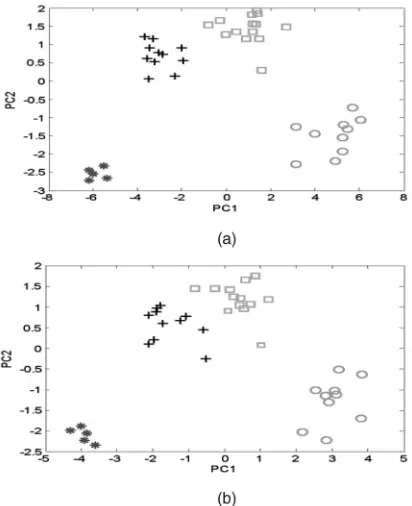
If the threshold for SERR is set to be 0.95, a subset of nine features should then be considered. To evaluate how well the 9-feature subset captures the structure of the complete data, a further principal component analysis was done on both the complete data and the data formed by the selected nine features. Fig. 1a presents the two-dimensional graph of the complete data matrix while Fig. 1b presents the two-dimensional representation of the 9-feature subset. Clearly, the 9-feature subset provides a satisfactory representation for the complete data providing that capturing the data structure is the prime objective. In Fig. 1a, both of the first two principal components (PCs) are functions of all the 19 variables, while in Fig. 1b, the first two PCs only involve the nine selected variables. Table 1 clearly shows which of these

individual variables contribute most and provides a ranked list of these. This aids interpretation because PCs in general cases are functions of all the original variables but FOS-MOD shows individual contributions.

Notice that Fig. 1 only graphically presents the performance of the FOS-MOD algorithm by qualitatively comparing the structure formed by the first two associated PCs. From this visual illustration, however, it is difficult to obtain a quantitive measure about how efficient the subsets selected by the FOS-MOD algorithm are. In the following, the FOS-MOD algorithm was thus applied to pattern classification by analysing several real data sets, to quantitively inspect the efficiency of the new algorithm.

3.2 Example 2—Data Sets from UCI Machine Learning

Repository

Five real data sets, taken from the UCI machine learning repository [27], are considered. The objective is to select a subset for each data set using the FOS-MOD algorithm and the selected subset is then used to replace the associated complete data for designed pattern classification. The threshold forSERRin the FOS-MOD algorithm was set to be 0.95 for all the five data sets. Details about the five data sets and associate experiments are given below:

. Wisconsin Breast Cancer (WBC). The Wisconsin breast

cancer data contains 699 samples, where 458 are benign samples (65.52 percent) and 241 are malignant samples (34.48 percent). Each instance is characterized by nine attributes. The objective is to predict diagnosis results that are either benign or malignant.

. Wisconsin Diagnostic Breast Cancer(WDBC). This data set

contains 569 samples, where 357 are benign samples (62.74 percent) and 212 are malignant samples (37.26 per-cent). Each instance is characterized by 30 real-valued attributes. The objective is as in the WBC data. . Johns Hopkins University Ionosphere. This data set contains

351 samples and 34 real-valued attributes. This data set involves a binary classification task.

TABLE 1

Feature Detection and Ranking Results for the Alate Adelges Data

. Cardiac Arrhythmia. This data set contains 452 instances and 279 attributes. The task is to classify a patient into one of the 16 classes of cardiac arrhythmia. This data set was preprocessed as below. Some values are missing for the attributes numbered by 11, 12, 13, and 15, and the missing values were filled with some values chosen randomly according to the distribution of the known values for the three attributes. Most of the values for the 14th attribute are missing and this attribute was not included in our experiment. Among the 279 attributes, 17 are trivial because all the observations for these attributes are zero. The 17 zero-valued attributes were not used in our experiment. . Forest Cover Type. This data set represents the forest cover

types in a region. There are 54 attributes, 581,012 instances and seven classes of cover types. The first 11,340 instances were used as the training data and the next 3,780 instances were used as the test data. Following [8], only the first 10 numerical-valued attributes were considered.

To inspect the performance of the new FOS-MOD algorithm, thek-nearest-neighbor (k-NN) algorithm was applied to evaluate the classification accuracy calculated by performing the following random cross-validation procedure. The k-NN algorithm was performed 20 times over the training and validation data defined as below: at each time, about 10 percent of the samples were randomly selected and left out, and these were used as the test data; the remaining 90 percent samples were used as the training data. The average classification accuracy of the 20 runs of thek-NN algorithm, over the test data, was then calculated. The value ofk, in thek-NN rule, was chosen by performing many experiments for different values ofk, where1k ffiffiffiffiffiffiffi_N

tr

p

andNtris the number of

the samples in the training set, andkwas chosen as the one that gives the best classification performance.

A feature subset for each of the five data sets, WBC, WDBC, Forest, Ionosphere, and Arrhythmia, was selected. The number of features in the selected subsets for the five data sets was 4, 13, 5, 19, and 96, respectively. Thek-NN algorithm was applied to both the original complete data and the associated feature subset for each of the five data sets. A comparison between the classification accuracy based on the complete data and the associated subset for the five data sets is reported in Table 2, where the associated algorithms are implemented using Matlab (R14) on a Sun-Blade-2500 workstation (1.28GHz ).

It can be seen from Table 2 that the classification accuracy based on the selected subsets is comparable with those based on the complete data. This means that the selected feature subsets are representative and informative and, thus, can be used to replace the complete data for pattern classification. Table 2 only presents the classification accuracy at some specific value ofk, where thek -NN rule provides the best classification performance. It may be informative to compare the overall classification accuracy for different values ofk, with respect to both the selected subset and the associated complete data. As a benchmark, Fig. 2 depicts such a comparison for the two data sets Forest and Arrhythmia.

For the data set WBC, the classification accuracy based on the selected subset is 97.42 percent, which is very near to the best result (97.5 percent) given in [28], where many classifiers were compared. For the data set WDBC, the classification accuracy based on the selected subset here is near to the result in [15], where the number of features involved in selected subsets is much more than the 13 used here. In this sense, the subset produced by the proposed algorithm for the data set WDBC is more compact. While for the data set Forest, the result produced by the FOS-MOD algorithm is comparable with those in [8], where several feature selection algorithms were compared, for the data sets Ionosphere and Arrhythmia, the results here are slightly better than those in TABLE 2

A Comparison of the Classification Accuracy over the Original Complete Data and the Associated Selected Subsets, Using thek-NN Algorithm

[8]. The mechanism of the FOS-MOD algorithm, however, is quite easy and the implementation of this algorithm only involves the calculation of the squared-correlation matrix and the maximization of the overall dependency. The results of the analysis of these data sets using several methods are already given in [8]. Comparing the results of the FOS-MOD algorithm with those in [8] therefore provides a full comparison of the various methods.

4

C

A new unsupervised learning algorithm has been proposed for feature selection and dimensionality reduction. The main advan-tage of the new algorithm is that the implementation only involves the calculation of the designed correlation matrix and the forward orthogonalization procedure. The new algorithm, which combines good effectiveness with high efficiency, often produces efficient feature subsets and, thus, provides an effective solution to the dimensionality reduction problem. The algorithm assumes that a linear relationship exists between sample features. In many cases, where features are linked by some nonlinear relationship, this assumption may become unreasonable. In such cases, more variables may need to be included in the final subset to achieve a satisfactory recognition result. This is a disadvantage of this type of approach. Future work will involve adapting the present method to accommodate nonlinear relationships and to seek more powerful dependence measurement criteria.

R

[1] M.A. Carreira-Perpinan, “Continuous Latent Variable Models for Dimen-sionality Reduction and Sequential Data Reconstruction,” PhD dissertation, Dept. of Computer Science, Univ. of Sheffield, Sheffield, U.K., 2001. [2] I.K. Fodor, “A Survey of Dimension Reduction Techniques,” Technical

Report UCRL-ID-148494, Lawrence Livermore Nat’l Laboratory, Center for Applied Scientific Computing, June 2002.

[3] A.K. Jain, R.P.W. Duin, and J. Mao, “Statistical Pattern Recognition: A Review,”IEEE Trans. Pattern Analysis and Machine Intelligence,vol. 22, no. 1, pp. 4-37, Jan. 2000.

[4] A.R. Webb,Statistical Pattern Recognition,second ed. Wiley, 2002. [5] I.T. Jolliffe,Principal Component Analysis,second ed. Springer, 2002. [6] G.P. McCabe, “Principal Variables,”Technometrics,vol. 26, pp. 137-144, May

1984.

[7] W.J. Krzanowski, “Selection of Variables to Preserve Multivariate Data Structure Using Principal Components,”Applied Statististics,vol. 36, no. 1, pp. 22-33, 1987.

[8] P. Mitra, C.A. Murthy, and S.K. Pal, “Unsupervised Feature Selection Using Feature Similarity,”IEEE Trans. Pattern Analysis and Machine Intelligence,

vol. 24, no. 3, pp. 301-312, Mar. 2002.

[9] B. Krishnapuram, A.J. Hartemink, L. Carin, and M.A.T. Figueiredo, “A Bayesian Approach to Joint Feature Selection and Classifier Design,”IEEE Trans. Pattern Analysis and Machine Intelligence,vol. 26, no. 9, pp. 1105-1111, Sept. 2004.

[10] M.H.C. Law, M.A.T. Figueiredo, and A.K. Jain, “Simultaneous Feature Selection and Clustering Using Mixture Models,” IEEE Trans. Pattern Analysis and Machine Intelligence,vol. 26, no. 9, pp. 1154-1166, Sept. 2004. [11] R. Kohavi and G.H. John, “Wrappers for Feature Subset Selection,”Artificial

Intelligence,vol. 97, nos. 1-2, pp. 273-324, Dec. 1997.

[12] A.J. Miller,Subset Selection in Regression.Chapman and Hall, 1990. [13] P. Pudil, J. Novovicova, and J. Kittler, “Floating Search Methods in Feature

Selection,”Pattern Recognition Letters,vol. 15, no. 11, pp. 1119-1125, Nov. 1994.

[14] S.K. Pal, R.K. De, and J. Basak, “Unsupervised Feature Evaluation: A Neuro-Fuzzy Approach,” IEEE Trans. Neural Networks, vol. 11, no. 2, pp. 366-376, Mar. 2000.

[15] K.Z. Mao, “Identifying Critical Variables of Principal Components for Unsupervised Feature Selection,”IEEE Trans. Systems, Man, and Cybernetics, Part B,vol. 35, pp. 339-344, 2005.

[16] I.T. Jolliffe, “Discarding Variables in a Principal Component Analysis-I: Artificial Data,”Applied Statistics,vol. 21, no. 2, pp. 160-173, 1972. [17] L. Breiman, “Statistical Modeling: The Two Cultures,”Statistical Science,

vol. 16, no. 3, pp. 199-215, Aug. 2001.

[18] Y. Amit and D. Geman, “Shape Quantization and Recognition with Randomized Trees,”Neural Computation,vol. 9, no. 7, pp. 1545-1588, Oct. 1997.

[19] Y. Amit, D. Geman, and K. Wilder, “Joint Induction of Shape Features and Tree Classifiers,” IEEE Trans. Pattern Analysis and Machine Intelligence,

vol. 19, no. 11, pp. 1300-1305, Nov. 1997.

[20] I. Guyon, J. Weston, S. Barnhill, and V. Vapnik, “Gene Selection for Cancer Classification Using Support Vector Machines,”Machine Learning,vol. 46, pp. 389-422, 2002.

[21] M. Korenberg, S.A. Billings, Y.P. Liu, and P.J. McIlroy, “Orthogonal Parameter Estimation Algorithm for Non-Linear Stochastic Systems,”Int’l J. Control,vol. 48, pp. 193-210, 1988.

[22] S.A. Billings, S. Chen, and M.J. Korenberg, “Identification of MIMO Non-Linear Systems Suing a Forward Regression Orthogonal Estimator,”Int’l J. Control,vol. 49, pp. 2157-2189, June 1989.

[23] T.M. Cover and J.M. Van Campenhout, “On the Possible Orderings in the Measurement Selection Problem,”IEEE Trans. Systems, Man, and Cyber-netics,vol. 7, no. 9, pp. 657-661, Sept. 1977.

[24] H.L. Wei, S.A. Billings, and J. Liu, “Term and Variable Selection for Nonlinear System Identification,”Int’l J. Control,vol. 77, no. 1, pp. 86-110, Jan. 2004.

[25] J.N.R. Jeffers, “Two Case Studies in the Application of Principal Component Analysis,”Applied Statistics,vol. 16, no. 3, pp. 225-236, 1967. [26] I.T. Jolliffe, “Discarding Variables in a Principal Component Analysis. II:

Real Data,”Applied Statistics,vol. 22, no. 1, pp. 21-31, 1973.

[27] D.J. Newman, S. Hettich, C.L. Blake, and C.J. Merz UCI Repository of Machine Learning Databases, http://www.ics.uci.edu/~mlearn/ MLRepository.html, 2006.

[28] Faculty of Physics, Dept. of Informatics, Nicolaus Copernicus Univ., Torun, Poland,http://www.phys.uni.torun.pl/kmk/projects/datasets.html, 2006.