Spatiotemporal analysis of an agent-based model of a colony of keratinocytes: a first approach for the development of validation methods

This is a repository copy of

Spatiotemporal analysis of an agent-based model of a colony

of keratinocytes: a first approach for the development of validation methods

.

White Rose Research Online URL for this paper:

http://eprints.whiterose.ac.uk/74613/

Monograph:

Pichardo-Almarza, C., Smallwood, R. and Billings, S.A. (2007) Spatiotemporal analysis of

an agent-based model of a colony of keratinocytes: a first approach for the development of

validation methods. Research Report. ACSE Research Report no. 955 . Automatic Control

and Systems Engineering, University of Sheffield

[email protected] https://eprints.whiterose.ac.uk/

Reuse

Unless indicated otherwise, fulltext items are protected by copyright with all rights reserved. The copyright exception in section 29 of the Copyright, Designs and Patents Act 1988 allows the making of a single copy solely for the purpose of non-commercial research or private study within the limits of fair dealing. The publisher or other rights-holder may allow further reproduction and re-use of this version - refer to the White Rose Research Online record for this item. Where records identify the publisher as the copyright holder, users can verify any specific terms of use on the publisher’s website.

Takedown

If you consider content in White Rose Research Online to be in breach of UK law, please notify us by

Spatiotemporal Analysis of an Agent-Based Model of a Colony of

Keratinocytes: A first Approach for the Development of Validation Methods

César Pichardo-Almarza

, Rod Smallwood

and S. A. Billings

1 University of Sheffield, Department of Computer Science, Sheffield S1 4DP, U.K.

2 University of Sheffield, Department of Automatic Control and Systems Engineering, Sheffield

S1 4DP, U.K.

E-mail:

[email protected]

,

[email protected]

,

[email protected]

Department of Automatic Control and Systems Engineering

The University of Sheffield, Sheffield, S1 3JD, UK

Research Report No. 955

Spatiotemporal Analysis of an Agent-Based Model of a Colony of

Keratinocytes: A first Approach for the Development of Validation Methods

César Pichardo-Almarza

, Rod Smallwood

and S. A. Billings

1 University of Sheffield, Department of Computer Science, Sheffield S1 4DP, U.K.

2 University of Sheffield, Department of Automatic Control and Systems Engineering, Sheffield

S1 4DP, U.K.

E-mail:

[email protected]

,

[email protected]

,

[email protected]

Abstract

Agent-based models are widely used for the simulation of systems from several domains (biology, economics, meteorology, etc). In biology agent-based models are very useful for predicting the social behaviour of systems; in particular they seem well adapted to model the behaviour of a cell population. In this paper an agent-based model, developed to study normal human keratinocytes (tissue cells), will be investigated. This kind of model exhibits probabilistic behaviour and the validation of simulation results is often done with a qualitative analysis by the experts (biologists). The main objective of this paper is to propose new variables and metrics that allow the comparison and a possible quantitative validation using numerical results from simulations.

1. Introduction

An agent-based computational model has been developed based on biological rules that govern the self-organization of normal human keratinocytes (NHK) [1]. This is the result of the combination of in vitro and in virtuo models used to explore the behaviour of NHK. The model helps to predict the dynamic multicellular morphogenesis of NHK and of a keratinocyte cell line (HaCat cells) under varying extracellular Ca++ concentrations. The model enables in virtuo exploration of the relative importance of biological rules and was used to test hypotheses in virtuo which were subsequently examined in vitro.

The agent-based model used in this work is composed of two parts: the agents, in this case the cells, and the environment, here being the culture dish

in which the cells reside, along with the global concentration level of calcium.

Each cell is modelled as a non-deformable sphere of 20µm in diameter. Cells are capable of migration, proliferation and differentiation. The culture is modelled as a flat, square surface with “walls” and the dimensions are user-defined. For the purposes of the experiments, the basement was 500µm in each dimension with a wall height of 100µm. The exogenous calcium level was set to 1.3mM (physiological calcium level) but the model can be used for different calcium levels (i.e., 0.1mM for the study of the system with a low calcium level).

Figure 1. Snapshots of simulations of the agent-based model

Results obtained from the model include the type of cell (stem, transit-amplifying (TA), committed or corneocyte) and their location. Each cell then performs specific rules associated with the cell cycle. Following this, cells decide whether to change to another cell type based on the differentiation rules in the model. Cells then execute their migration rules,

k _{= 0 iterations} k _{= 400 iterations}

and finally execute physical rules. All rules are executed in the context of the agent’s own internal state and the states of the other cells around it.

The computational model allows the user to access several variables associated with each cell in the dish (position, type, number of intercellular bonds, etc) for each iteration k. Mean cell cycle time and migration rate are scaled so that each time step in the model represents approximately 30 min in real time. For the purpose of this paper, the dynamical response of the spatial location of each cell was the main variable.

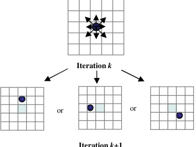
When a simulation is performed, the first observations that are available to the user are that individual cells can move in any direction from time k

to time k+1 (Figure 2).

Figure 2. Possible scenarios for iteration k+1

This kind of reaction generates a stochastic behaviour for the whole cell population.

The analysis of the development of spatial distribution in stochastic processes where both type and position of the objects is involved has not been extensively developed in the literature. This kind of study is an important and necessary procedure for the validation of these models. The spatiotemporal analysis is particularly relevant to the understanding of the development of properly structured and functional tissue in multi-cellular organisms.

Figure 2 shows that the same migration behaviour could be considered as different for several experiments if a classic spatial analysis (i.e. discretizing the dish with a 2D square grid) is used to study the spatial distribution of cells. A cell can migrate to any case around its original location, thus, if a square grid is used, an occupied case in a given experiment could be empty in another experiment.

Because of this effect, a circular approach, based on concentric circles around the centre of the dish (x = 250, y = 250) will be introduced. In this particular

analysis 12 circles with a radius variation of 30µm were employed (Figure 3).

(a) (b)

Figure 3. (a) Initial location of cells; (b) circular grid

Once the grid is defined, the objective is to calculate several variables associated with the spatial behaviour of the cell population. The calculation of these variables is made in each ring of the circular grid.

2. Defining quantitative variables for

comparison

The first variable to be calculated is the number of cells in each ring of the grid. This will give information about the spatial distribution of the cells. Two variables were selected to evaluate the migration of cells: positive migration and negative migration. Positive migration is the number of cells entering the ring and negative migration represents the number of cells leaving the ring. Finally the mitosis is calculated as the number of cells in the ring because of the division of cells. These effects will be discussed in more detail in the following sections.

2.1 Comparing the spatial distribution of cells

The spatial distribution can be evaluated as the variation of the total number of cells in each ring. With that objective in mind a vector with n rows (n = number of radii used in the circular grid) is built for each iteration k:

     

 

     

 

=

) (

) 1 (

Rn R1

n NCell NCell

NCell

k k

k M

(1)

2.2 Comparing Migration

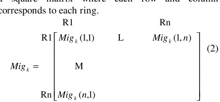
The criterion to evaluate the migration of cells is observing the number of cells that move from ring “j” to ring “i”. This behaviour can be achieved by filling

Iteration k₊₁

or or

a square matrix where each row and column corresponds to each ring.

                = ) 1 , ( ) , 1 ( ) 1 , 1 ( Rn R1 Rn R1 n Mig n Mig Mig Mig k k k k M L (2)

The element (i, j) of the Migk matrix for each

iteration corresponds to the number of cells that migrate from ring “i” to ring “j”. Obviously the element (i, i) is the number of cells that remain in the ring “i”. In general, there will be a transfer of cells from/to ring “i” to/from ring “i+1” and “i-1”, which means that a tridiagonal matrix is obtained at each iteration.

Figure 4. Circular grid: evaluating Migration and Mitosis

To calculate the total number of cells at time “k” in ring “i”, a simple equation based on migration (from and to ring “i”) and mitosis can be used.

i k C = i

k

C−1+Minki−1−Moutki−1+Mitki−1 (3)

Where i k

C is the total number of cells in ring “i” at time k, i

k

C−1 is the total number of cells in ring “i” at

time k-1, i k

Min ₋₁ is the number of cells that migrated from other rings to ring “i”, i

k

Mout −1 is the number of

cells that migrated from ring “i” to other rings and i

k

Mit₋₁ is the number of new cells in ring “i” because of mitosis.

To compare migration the terms i k

Min and Moutik for each ring “i” can be evaluated. These terms are useful for calculating the “migratory” flow of cells; the objective is to evaluate the variation of the number of cells in ring “i” ( i

k

C ) because of Minkiand i k Mout . To illustrate this effect assume that the total number of cells in ring “i” varies only because of the migration of cells from other rings,

i k C = i

k

C₋₁ i k Min ₋₁

+ (4)

Alternatively the total number of cells varies only because of the migration of cells from ring “i” to other rings,

i k C = i

k

C₋₁ i

k Mout ₋₁

− (5)

Equations (4) and (5) can be used to compare the migration in each ring. The positive migration in ring “i” ( i

k

PM ) can then be defined as: i

k

PM = i

k

PM ₋₁ i k Min₋₁

+ (6)

and the negative migration i k NM −1as:

i k

NM = i

k

NM −1−Moutki−1 (7)

The term i k

Min₋₁corresponds to the sum of the elements (i-1, i) and (i-1,i) of matrix i

k

Mig −1 (equation

8) and i k

Mout ₋₁ corresponds to the sum of elements (i,

i+1) and (i,i-1) of matrix i k

Mig −1 (equation 9).

) , 1 ( ) , 1 (

1 Mig i i Mig i i

Min k k

i

k− = + + − (8)

) 1 , ( ) 1 , (

1= + + −

− Mig i i Mig i i

Mouti _{k k}

k (9)

2.3 Comparing Mitosis

The same circular grid can also be used to evaluate the mitosis of cells in the dish (Figure 3b). Equation (3) can be used to calculate the term associated with mitosis ( i

k Mit ₋₁):

i k Mit −1=

i k C −Cki−1

i k Min ₋₁

− i

k Mout −1

+ (10) This will yield a vector for each iteration, thus if there are “n” radii, Mitkwill have n components:

          = n k k k M M Mit M 1 (11)

Using a similar reasoning, a method to compare mitosis in each ring can be developed. This can be used to evaluate how the number of cells in ring “i” (

C

“k”. Assuming that the total number of cells in ring “i” varies only because of mitosis in this ring, gives

i k C = i

k C₋₁ i

k Mit ₋₁

+ (12)

Defining i k

RMit ₋₁ as the Mitosis rate in ring “i”, i

k

RMit −1= Cki−1+Mitki−1 (13)

produces a variable which can be used to compare mitosis in different simulations.

2.4 Using statistics to compare results

i k

Min

i k

As a first approach, the main objective of this paper is to propose accessible techniques to allow a quantitative comparison between the results from two (or several) simulations of the agent-based model. The purpose is to try to extend these methods for the validation of results of the agent-based model with experimental results obtained from the in vitro model. Results from two simulations using the same parameters and initial conditions can be compared using classical statistical techniques, i.e., linear regressions, etc. Future work could include the use of specialized tools for the statistical analysis of circular data [2,3].

With the variables proposed in this paper a dynamical evolution in time is obtained for the different radii of the grid, thus classical statistics can be used to compare this dynamical response from two simulations. The method to calculate the variables and a statistical analysis to compare simulation results are illustrated in the following example.

3. Example

In this example a comparison between the dynamical responses of two simulations is shown. In this case both simulations use the same initial positions of cells and parameters (calcium levels, etc). Simulations are generated using physiological calcium level (1.3 mM) and 8 initial cells in the dish with different spatial locations (Figure 3a).

The spatial distribution, mitosis and migration are compared using the techniques proposed in sections above.

3.1 Spatial distribution

The vectors associated with the spatial distribution of cells from these two simulations (NCell) will be obtained. The main idea is to find this vector for each iteration observing if the number of cells in each ring is similar in both simulations. For example, when the

NCell vector is calculated for iteration 1000, the following results are obtained:

NCell1000

(Simulation 1)

NCell1000

(Simulation 2)

11 40 57 74 93 110 137 144 122 59 24 7

8 25 38 64 101 123 133 147 123 50 20 7

To compare these vectors a linear regression can be applied, observing the number of cells in each ring. A regression factor (R) equal to 0.98 and a constant of the linear model (B; Y = BX) equal to 0.94 are obtained for this iteration.

(a) (b)

Figure 5. Spatial distribution: (a) Correlation factor,

R; (b) Linear coefficient, B

Calculating the NCell vector for each iteration and the linear correlation between the elements of both simulations, the obtained values of R and B are very close to 1. Figures 5 shows the temporal evolution of R

and B.

3.2 Migration

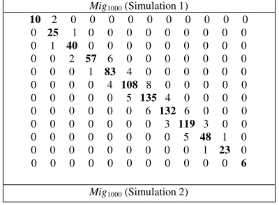
The migration of cells is evaluated using the circular grid of Figure 3b. Calculating the migration matrix at iteration 1000, the following results are obtained:

Mig1000 (Simulation 1)

10 2 0 0 0 0 0 0 0 0 0 0 0 25 1 0 0 0 0 0 0 0 0 0 0 1 40 0 0 0 0 0 0 0 0 0 0 0 2 57 6 0 0 0 0 0 0 0 0 0 0 1 83 4 0 0 0 0 0 0 0 0 0 0 4 108 8 0 0 0 0 0 0 0 0 0 0 5 135 4 0 0 0 0 0 0 0 0 0 0 6 132 6 0 0 0 0 0 0 0 0 0 0 3 119 3 0 0 0 0 0 0 0 0 0 0 5 48 1 0 0 0 0 0 0 0 0 0 0 1 23 0 0 0 0 0 0 0 0 0 0 0 0 6

Mig1000 (Simulation 2)

Iterations Iterations

10 0 0 0 0 0 0 0 0 0 0 0 1 31 0 0 0 0 0 0 0 0 0 0 0 0 42 6 0 0 0 0 0 0 0 0 0 0 2 59 3 0 0 0 0 0 0 0 0 0 0 4 83 10 0 0 0 0 0 0 0 0 0 0 3 102 1 0 0 0 0 0 0 0 0 0 0 5 126 3 0 0 0 0 0 0 0 0 0 0 3 131 3 0 0 0 0 0 0 0 0 0 0 3 111 2 0 0 0 0 0 0 0 0 0 0 2 35 2 0 0 0 0 0 0 0 0 0 0 1 17 1 0 0 0 0 0 0 0 0 0 0 1 4

As mentioned before, the elements on the diagonal of matrices Migk are the number of cells that remain

(from iteration k-1) in each ring. Thus, the evaluation of the positive migration is made by taking the elements of Migk in position (i+1, i) and (i-1, i) and

the evaluation of the negative migration is made by taking the elements of Migk in position (i, i-1) and (i,

i+1).

) , 1 ( ) , 1 (

1 Mig i i Mig i i

Mini _{k k}

k− = + + − (8)

) 1 , ( ) 1 , (

1= + + −

− Mig ii Mig ii

Mout k k

i

k (9)

For example, drawing the temporal evolution of the positive and the negative migration for rings 5 and 8 Figures 6 and 7 are obtained respectively.

(a) (b)

Figure 6. (a) Positive migration for ring 5; (b) Negative migration for ring 5

(a) (b)

Figure 7. (a) Positive migration for ring 8; (b) Negative migration for ring 8

Figures 6 and 7 show that the dynamical response of the positive and negative migration for both simulations are very similar. The same procedure can be applied for all rings and a similar behaviour will be obtained.

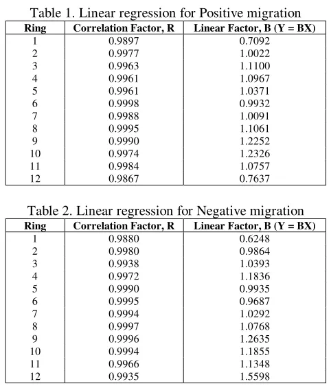
Tables 1 and 2 show the results of R and B of a linear regression between the results of both simulations:

Table 1. Linear regression for Positive migration

Ring Correlation Factor, R Linear Factor, B (Y = BX)

1 0.9897 0.7092

2 0.9977 1.0022

3 0.9963 1.1100

4 0.9961 1.0967

5 0.9961 1.0371

6 0.9998 0.9932

7 0.9988 1.0091

8 0.9995 1.1061

9 0.9990 1.2252

10 0.9974 1.2326

11 0.9984 1.0757

12 0.9867 0.7637

Table 2. Linear regression for Negative migration

Ring Correlation Factor, R Linear Factor, B (Y = BX)

1 0.9880 0.6248

2 0.9980 0.9864

3 0.9938 1.0393

4 0.9972 1.1836

5 0.9990 0.9935

6 0.9995 0.9687

7 0.9994 1.0292

8 0.9997 1.0768

9 0.9996 1.2635

10 0.9994 1.1855

11 0.9966 1.1348

12 0.9935 1.5598

3.3 Mitosis

In this case, the evaluation of mitosis in each ring is made using the circular grid of Figure 3b and equation (13).

i k

RMit −1= Cki−1+Mitki−1 (13)

With this equation the mitosis rate for both simulations is obtained. Figure 8 shows an example of the evolution of mitosis in time for ring 5 and ring 8. Similar results are obtained for the other radii. Table 3 shows the values of the linear correlation (R and B) between migration results of both simulations.

(a) (b)

Figure 8. (a) Mitosis rate in ring 5; (b) Mitosis rate in ring 8

Table 3. Linear regression for Mitosis

Ring Correlation Factor, R Linear Factor, B (Y = BX)

1 0.9915 0.8282

2 0.9969 0.92969

3 0.9984 0.8656

Iterations Iterations

Iterations Iterations

4 0.9991 1.1706

5 0.9992 0.96496

6 0.9997 1.0133

7 0.9998 1.06

8 0.98894 0.99933

9 0.99962 1.1045

10 0.9971 1.0419

11 0.99441 1.1697

12 0.92399 3.0375

4. Monte Carlo Simulations

Because of the probabilistic behaviour of the agent-based model used to simulate the behaviour of NHK, there is a possibility of obtaining different responses for two simulations (using the same set of parameters). A good method which allows the evaluation of the behaviour of a random process is Monte Carlo Simulations.

Monte Carlo (MC) methods are statistical simulation methods, using random numbers to give approximate solutions to mathematical problems. Developed by Neumann [4], Ulam [5] and Metropolis [6] during World War Two, this method has been used to model a large variety of problems, from the estimation of pi [8] to immune system simulation [9,10].

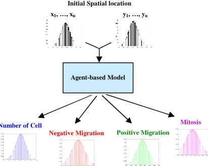
In the particular case of this work MC simulations are used to observe the behaviour of the agent-based model. The procedure consisted of running 100 simulations of the model. For each simulation a set of random positions (x, y) with a normal distribution were generated. After each simulation a dynamic response of the variables defined to evaluate the spatial behaviour of cells (number of cells, positive and negative migration and mitosis) was obtained. Finally the results of the 100 simulation were analysed using statistical tools.

Figure 9. Block diagram for the MC simulations

4.1 Analyzing the Monte Carlo Simulation Results

Classical statistics can be used to interpret the results of Monte Carlo simulations. The main idea is to calculate some statistical variables for the evaluation and testing of the model. In this paper, classical tools have been selected to evaluate the dynamic simulation results. The main objective of this statistical analysis is to determine whether similar behaviours are obtained for several simulations under similar conditions and parameter values.

In this case, the mean value, standard deviation and confidence intervals were calculated for each iteration. After these calculations a “mean” dynamical response is obtained for each variable with additional information about the temporal evolution of the confidence intervals.

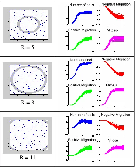
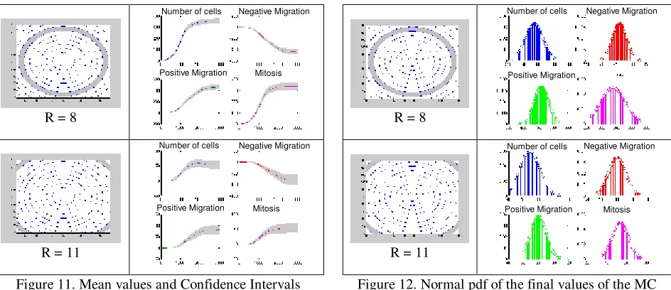
Additionally to evaluate the probability of obtaining similar final values of the simulations a probability density function (pdf) was calculated at each radius. Figures 10 and 11 show the simulation results, the mean value and the confidence intervals for several radii in the grid. Figure 12 shows the normal pdf for the final values of number of cells, negative migration, positive migration and mitosis.

These results show similar behaviours for several simulations using similar conditions. The confidence intervals were consistent with the dynamical behaviour of the cell population: a more random behaviour is obtained in small areas (i.e., the centre and the corner of the dish), thus larger confident intervals are obtained for these radii. However, the obtained normal pdf’s indicate that the results from simulations had the highest probability to be near the mean values.

Ring in the grid MC Simulation Results

R = 3

x1, …, xn y1, …, yn

Agent-based Model

Number of Cell

Negative Migration Positive Migration Initial Spatial location

Mitosis

Number of cells Negative Migration

R = 5

R = 8

R = 11

Figure 10. MC Simulation results

5. Conclusions

This work is a first approach for the spatiotemporal analysis of an agent-based model of NHK. This analysis represents an important contribution for the study of the spatial distribution in stochastic processes where both type and position of the objects is involved. This kind of study is an important and necessary procedure for the validation of these models. A good method for the spatiotemporal analysis is particularly relevant to the understanding of the development of properly structured and functional tissue in multi-cellular organisms.

The new variables defined in this paper allow more spatiotemporal information to be obtained from the computational model of NHK; these variables represent useful measurements in quantitative comparisons.

The methods developed, allow a quantitative comparison of two simulations with respect to the spatial distribution of cells, how the cells move in the dish (migration) and the reproduction of cells (mitosis) using classical statistics methods.

The spatial distribution has been compared by building a vector for each iteration with the number of cells in each ring of the grid. Thus, a linear

regression can be calculated and a temporal evolution of the correlation factors can be obtained.

Migration has been compared by observing how cells move from one ring to another. In this case, the “positive” and the “negative” migration can be compared in each ring for the total simulation time. Mitosis is compared using a method very similar to the migration method and simulations can be compared using a “Mitosis rate”.

In this work the behaviour of cells was analysed using the same calcium level (physiological calcium level). However, the calcium level is a parameter which can have a large influence on the behaviour of the cell population [11]. Future research will include similar spatiotemporal analysis concerning the variation of this parameter and the influence on the dynamical response of the agent-based model.

Algorithms are being formulated in Matlab [12] for application in the analysis and comparison of data from different models and/or different experiments. The results obtained from this work are encouraging and it is expected that they will be useful in comparing experimental results from an accurate cell tracking system which is currently under development as part of the Epitheliome project [13].

Ring in the grid Mean value and Confidence Limits

R = 3

R = 5

Number of cells

Number of cells

Number of cells

Negative Migration

Negative Migration

Negative Migration

Mitosis Mitosis

Mitosis Positive Migration

Positive Migration

Positive Migration

Number of cells Negative Migration

Mitosis Positive Migration

Number of cells Negative Migration

R = 8

R = 11

Figure 11. Mean values and Confidence Intervals obtained for the MC simulations

6. Acknowledgement

The authors gratefully acknowledge support from the Engineering Physical Sciences Research Council (EPSRC) for Doctor Pichardo for this project. Also the authors have to express a special acknowledge to Dr Sun Tao and Dr Phil Mcminn for giving support with the computational and in vitro models of NHK.

Ring in the grid Final Values (Normal pdf)

R = 3

R = 5

R = 8

R = 11

Figure 12. Normal pdf of the final values of the MC simulations

7. References

[1]T. Sun, P. McMinn, S. Coakley, M. Holcombe, R. Smallwood, S. MacNeil, “An Integrated Systems Biology Approach to Understanding the Rules of Keratinocyte Colony Formation”. Journal of the Royal Society Interface, To Appear, 2007.

[2] Fisher, N.I, Statistical analysis of circular data, Cambridge University Press. Cambridge, 1993.

[3] Jammalamadaka, S. Rao and A. SenGupta, Topics in circular statistics. World Scientific Publishing. Singapore, 2001.

[4] J.V. Neumann, in: A.W. Burks (Ed.), Theory of Self-Reproducing Automata, University of Illinois Press, Champaign, IL, 1966.

[5] N. Metropolis, S. Ulam, “The Monte Carlo method”, J. Am. Stat. Assoc. 44 ,1949, 335–341.

[6] N. Metropolis, “The beginning of the Monte Carlo method”, Los Alamos Sci. 15, 1987, 125.

[7] J.M. Hammersley, D.C. Handscomb, Monte Carlo Methods, Chapman & Hall, New York, 1964.

[8] J.H. Mathews, Monte Carlo Estimate for Pi, Pi Mu Epsilon J., 5, 1972, 281–282.

[9] S. Dasgupta, “Monte Carlo simulation of the shape space model of immunology”, Physica A: Stat. Theor. Phys. 189 (3–4), 1992, 403–410.

[10] R. Mannion, H.J. Ruskin, R.B. Pandey, “Effects of viral mutation on cellular dynamics in a Monte Carlo simulation of HIV immune response model in three dimensions”, Theory Biosci., 121 (2), 2002, 237–245. [11] Walker D, Sun T, Macneil S, Smallwood R,

“Modeling the Effect of Exogenous Calcium on Keratinocyte and HaCat Cell Proliferation and Differentiation Using an Agent-Based Computational Paradigm". Tissue Eng., 12(8), 2006, 2301-2309 [12] The Mathworks, Inc., http://www.mathworks.com

Number of cells Negative Migration

Mitosis Positive Migration

Number of cells Negative Migration

Mitosis Positive Migration

Number of cells Negative Migration

Mitosis Positive Migration

Number of cells Negative Migration

Mitosis Positive Migration

Number of cells Negative Migration

Mitosis

Positive Migration

Number of cells Negative Migration