Null Models and Dispersal Distributions: A Comment on an Article by Caley

(1)

This is a repository copy of

Null Models and Dispersal Distributions: A Comment on an

Article by Caley

.

White Rose Research Online URL for this paper:

http://eprints.whiterose.ac.uk/1405/

Article:

Rees, M. (1993) Null Models and Dispersal Distributions: A Comment on an Article by

Caley. American Naturalist, 141 (5). pp. 812-815. ISSN 0003-0147

[email protected] https://eprints.whiterose.ac.uk/

Reuse

Unless indicated otherwise, fulltext items are protected by copyright with all rights reserved. The copyright exception in section 29 of the Copyright, Designs and Patents Act 1988 allows the making of a single copy solely for the purpose of non-commercial research or private study within the limits of fair dealing. The publisher or other rights-holder may allow further reproduction and re-use of this version - refer to the White Rose Research Online record for this item. Where records identify the publisher as the copyright holder, users can verify any specific terms of use on the publisher’s website.

Takedown

If you consider content in White Rose Research Online to be in breach of UK law, please notify us by

(2)

Vol. 141, No. 5 The American Naturalist May 1993

N U L L MODELS AND DISPERSAL DISTRIBUTIONS: A COMMENT ON AN ARTICLE BY CALEY

In a recent article Caley (1991) outlined a null model for dispersal distributions against which he suggested empirical data should be compared. He first presented Waser's geometric model (Waser 1985), which can be derived as follows: Dispers- ing individuals move in a straight line from the natal site and settle in the first unoccupied site they encounter. If unoccupied sites occur independently at ran- dom with probability t as a result of turnover within the habitat, then the distribution of dispersal distances will follow a geometric distribution in which the probability of settling at distance i is given by

p(i) = t(l - t)' f o r i = 0, 1 , 2 , 3 , .

.

. ₍₁₎

Note that distance traveled in this model is measured in terms of the mean size of the home range and that the natal site is designated site 0. In this model individual dispersal behavior is deterministic, in the sense that individuals settle with probability l at the first unoccupied site they encounter. Thus, if we know the distribution of occupied and unoccupied sites and the direction in which an individual is dispersing, then we know exactly how far the individual will travel. Caley suggests that when this model is applied, a null model should also be fitted in order to determine which provides the best description of the data. The null model suggested by Caley is the exponential distribution for which the probability density function is

This distribution is derived by assuming that the probability that an individual will settle in the next short interval, Ax, is approximately PAX, which is independent of the distance traveled, X . It is also assumed that individual dispersal dis-

tances are statistically independent. Note that in this model it is the stochasticity in individual behavior in a homogeneous environment that generates the observed distribution of dispersal distances. In contrast, the geometric model assumes individual behavior is deterministic (see above) and that stochasticity in the environment (i.e., the presence of occupied and unoccupied sites) generates the dispersal distribution.

The main problem with Caley's approach is that the geometric distribution and the appropriate discrete form of the exponential distribution are, in fact, identical.

Am. Nat. 1993. Vol. 141, pp. 812-815.

(3)

N O T E S A N D C O M M E N T S 813

To see this, note that in order to form a discrete distribution from the exponential distribution we integrate over each home range

1 b 1

p(i) = Pe P'dx f o r i = 0, l , ? ,

.

Now p(0) = 1 - r P P , which is t in the geometric model. Substituting for t = 1

- in equation (1) gives equation (2), demonstrating the equivalence of the

two distributions. This equivalence arises because in both models the probability of an individual's settling is independent of the distance traveled (i.e., the distance-specific rate of settling is a constant). Given this equivalence, it is difficult to see how Caley obtains the results presented in his figure 1, in which the two distributions appear very different. What it appears Caley has done is to equate the mean of the geometric distribution to the mean of the continuous exponential distribution in order to obtain the value of

P

for the exponential model, giving

p

= tl(1 - t). Using this procedure, I have been able to obtain Caley's figure 1A and B, but not C, which appears to be incorrectly drawn. What Caley should have done is to solve t = 1 - r-B for p, giving

P

= -ln(l - 1 ) : when this expression is used, the probability distributions are identical.

In order to obtain parameter estimates, Caley equates the observed mean dispersal distance to the mean of the theoretical distribution being fitted. A far better approach would be to use maximum likelihood estimation methods (Cox and Oakes 1984); these allow explicit tests of exponentiality (Cox and Oakes 1984, p. 43) and departures from exponentiality to be characterized. In an earlier article, a collcaguc and I (Rccs and Long 1993) give a biological examplc that allows for discreteness in the data and truncation.

(4)

814 T H E AMERICAN NATURALIST

Distance

[image:4.495.93.398.87.332.2]

Type 1 Type 2 Population

... -

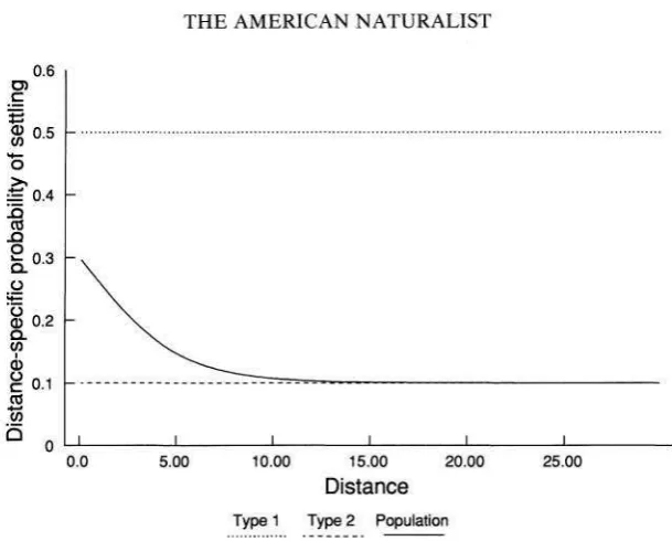
FIG. 1 .-Distance-specific rate of settling a s a function of the distance traveled for individuals of types 1 and 2, each of which disperse according to an exponential distribution, and for a population initially composed of equal proportions of each type. Parameter values: 6,

= 0.5, ( j 2 = 0 . 1 , ~ = .5.

the distance traveled. The population-level distance-specific rate of settling, h ( x ) , is

where

p ,

and

p,

define the exponential dispersal distributions for individuals of types I and 2 , respectively. Note that if p = 1 then h ( x ) =

p,,

whereas if p = 0

then h ( x ) =

p,.

So, if there is no between-individual variability then the probability of settling is independent of the distance traveled. The initial rate of settling is h(0) =

p p ,

+

(1

+

p)P,,

whereas as X

-.

m, h ( x ) +

p ,

if

P, < P,,

or h ( x )

-.

p,

if

PI

>

p,.

Thus, initially the distance-specific settling rate is simply the average of the two types present in the population. However, at greater dispersal distances the population becomes dominated by those individuals with the lower

P.

(5)

NOTES AND COMMENTS

ACKNOWLEDGMENTS

I would like to thank M. J . Caley, M. J. Crawley, M. J. Long, and K. Shea for helpful comments on the manuscript.

1,ITEKATUKE CITED

Caley, M. J. 1991. A null model for testing distributions of dispersal distances. American Naturalist 138:524-532.

Cox, D. R., and D. Oakes. 1984. Analysis of survival data. Chapman & Hall, London. Pielou, E . C. 1977. Mathematical ecology. Wiley, London.

Kees, M., and M. J. Long. 1993. The analysis and interpretation of seedling recruitment curves. American Naturalist 141:233-262.

Vaupel, W . V., K. G. Manton, and E. Stallard. 1979. The impact of heterogeneity in individual frailty on the dynamics of mortality. Demography 16:439-454.

Waser, P. M. 1985. Does competition drive dispersal? Ecology 66:1170-1175.

MARK REES DEPARTMENT OF BIOLOGY A N D CENTRE FOR POPULATION BIOLOGY

IMPERIAL COLLEGE, SILWOOD PARK

ASCOT, BERKSHIRE, SLg 7PY UNITED KINGDOM

Submitted December 10, 1991; R e v i ~ e d June 1, 1992; Accepted June 15, 1992