Maximum Likelihood Estimation of Higher-Order
Integer-Valued Autoregressive Processes
Ruijun Bu, Brendan McCabe
The University of Liverpool
Kaddour Hadri
Durham University
Final Version
(April 2008)
Maximum Likelihood Estimation of Higher-Order
Integer-Valued Autoregressive Processes
Abstract
In this paper, we extend earlier work of Freeland and McCabe (2004) and develop a general framework for maximum likelihood (ML) analysis of higher-order integer-valued autoregressive processes. Our exposition includes the case where the innovation sequence has a Poisson distribution and the thinning is Binomial. A recursive represen-tation of the transition probability of the model is proposed. Based on this transition probability, we derive expressions for the score function and the Fisher information ma-trix, which form the basis for maximum likelihood estimation and inference. Similar to the results in Freeland and McCabe (2004), we show that the score function and the Fisher information matrix can be neatly represented as conditional expectations. Using the IN AR(2) speci…cation with Binomial thinning and Poisson innovations, we examine both the asymptotic e¢ ciency and …nite sample properties of the ML estimator in relation to the widely used conditional least squares (CLS) and Yule-Walker (YW) estimators. We conclude that, if the Poisson assumption can be justi…ed, there are substantial gains to be had from using ML especially when the thinning parameters are large.
1. Introduction
Recently there has been growing interest in modeling time series of small counts that arise in various …elds of statistics. Examples include the number of customers waiting to be served at a counter recorded at discrete points in time; the daily number of absent workers in a …rm; the monthly cases of rare infectious diseases in a speci…ed area; the monthly number of claimants collecting wage loss bene…t for injuries in the workplace and so on. Typically, such time series take on only small non-negative integer values and often exhibit short-range dependence. Traditional continuous variable models are apparently inappropriate in that they would in-variably produce non-integer forecast values. As a result, some speci…c class of time series models has to be entertained to explicitly account for the discreteness. This paper is concerned with a special class of observation-driven models called integer-valued autoregressive processes introduced independently by Al-Osh and Alzaid (1987) and McKenzie (1988). In this paper we use the notationIN AR(p) to mean that the thinning operator (withplags) of the process is Binomial while the discrete innovations process is left unspeci…ed. When the innovations process is speci…ed to be Poisson then we write IN AR(p)-P. If neither the thinning nor the innovations processes are fully speci…ed we use the generalised GIN AR(p) notation.
method. The main contribution of the present paper is to extend earlier work and develop a general framework for likelihood analysis of higher order GIN AR(p) processes with general thinning operators and innovation distributions. We de-rive the likelihood, using a recursive formulation of the transition probabilities, which facilitates both numerical computations and the derivative calculations re-quired for the score and information quantities. Similar to the results in FM, we show that all elements of the score and the Fisher information matrix can be rep-resented in terms of conditional expectations which enhances the interpretation of these quantities. While the results are quite general, we also specialise to the situation where the thinning processes are Binomial and the innovation sequence is Poisson and provide speci…c formulae for computational use in this case. The additional distributional assumptions also allow for veri…able conditions to en-sure the existence of asymptotic stationary and limit distributions for the process and associated estimators. We also investigate the asymptotic relative e¢ ciency (ARE) of CLS to ML and these calculations show that there are quite substantial e¢ ciency gains to be had by imposing the Poisson assumption (should it be jus-ti…ed) especially when the thinning parameters are large in magnitude. A Monte Carlo study shows that ML also has advantages in small samples in terms of bias and mean squared error (MSE).
The remainder of the paper is organized as follows. Section 2 presents a like-lihood framework for theGIN AR(p)model and derives the likelihood, score and information. In Section 3, we outline theIN AR(p)-P process and brie‡y review its main statistical properties. In Section 4, the asymptotic relative e¢ ciency of the ML estimator is examined and a simulation experiment looks at the small sample properties. Section 5 concludes. The proofs and other details are contained in Appendices.
2. Likelihood Calculations for the
GIN AR
(
p
)
Model
In this section we consider aGIN AR(p) model where the thinning operators and arrivals distribution are speci…ed in just enough detail to enable the likelihood and the associated score and information to be calculated. Additional assumptions are needed to ensure enough regularity for maximum likelihood estimators to be asymptotically normal, for example1. The variableX
tis assumed to be generated
1We do not pursue, here, abstract conditions for the MLE in the GIN AR(p) model to be
according to
Xt= 1 Xt 1+ 2 Xt 2 + + p Xt p+"t (1)
where, conditional onXt k, k Xt kis an integer-valued random variable (random operator) with parameter k2. The variables k Xt k, k2 f1; :::; pg, conditional onXt k, k 2 f1; :::; pg, are mutually independent. The operator thus delivers an integer value and dependence in fXtg is induced via the conditioning variables Xt k,k 2 f1; :::; pg. The operator k Xt k may correspond to Binomial thinning and with "t a Poisson variable this gives rise to the standardIN AR(p)-P model; whenp= 1,Xthas a Poisson distribution. Other possibilities are that conditional on Xt k, k Xt k is Beta-Binomial while "t is Negative Binomial; when p = 1 this will ensure thatXtis also Negative Binomial. For a general treatment of such operators see Joe (1996). The conditional probability density function of k Xt k givenXt k, with respect to the counting measure , is written
f(skjXt k; k) (2)
while that of"t is
g("; ): (3)
In the calculations required for the score and the information matrix we assume that these densities satisfy
@f(skjXt k; k) @ k
= (sk;Xt k; k)f(skjXt k; k)
@g("; )
@ = ("; )g("; )
(4)
where ( ) and the vector function ( ) are di¤erentiable with respect to the parameters.
The next two sub-sections look at a likelihood based analysis of theGIN AR(p) model. We condition on the …rstpobservations3. The …rst sub-section looks at the conditional likelihood while the second treats the score and information quantities.
2In fact,
k may be a vector but we stick to the simpler scalar notation.
3The full likelihood may, however, be computed under stationarity as P(X
1; ::; Xp)may be
2.1. The Conditional Likelihood
Conditioning on the …rst p observations leads to a simple form of the likelihood viz.
L( 1; : : : ; p; ) = T
Y
t=p+1
P(XtjXt 1; : : : ; Xt p) (5)
and so knowledge of the transition probabilities is su¢ cient for its construction. Theorem 2.1 below shows how these conditional probabilities may be calculated by a simple recursive mechanism. The idea is to regard Xt as the convolution of
1 Xt 1 and 2 Xt 2 + + p Xt p+"t, which are by de…nition mutually independent given thepobserved lags. Then 2 Xt 2+ + p Xt p+"tmay be thought of the the convolution between 2 Xt 2 and 3 Xt 3+ + p Xt p+"t and this leads to an obvious recursion.
Theorem 2.1. In the model (1)
P(XtjXt 1; : : : ; Xt p)
=
Z
f(s1jXt 1)P(Xt s1jXt 2; : : : ; Xt p)d (s1) (6)
where the starting value is given by
P Xt p 1
X
k=1
sk Xt p
!
=
Z
f(spjXt p)g Xt p 1
X
k=1
sk sp
!
d (sp): (7)
Theorem 2.1 allows the conditional likelihood of the GIN AR(p) model (1) to be calculated for any innovations sequencef"tg and thinning variables via (5). In addition to facilitating computation of the (conditional) likelihood, the recursions of Theorem 2.1 are also very useful in computing derivatives and hence the score and information quantities.
2.2. The Score and Information
Theorem 2.2. Let `_ k denote the score with respect to k for k 2 f1; :::; pg
and `_ the score with respect to the vector . Denote by Et[ ] the conditional
expectation with respect to the sigma …eld, =t = Xt; Xt 1; :::; Xt p . Assume
the density functions f and g in (2) and (3) satisfy (4). Then for the model (1)
_ ` k =
T
X
t=p+1
Et[ ( k Xt k)]
and
_ ` =
T
X
t=p+1
Et[ ("t)]
where ( k Xt k) = ( k Xt k;Xt k; k) and ("t) = ("t; ).
It is important to note that the time t expectations are di¤erent from those calculated at time t 1.
The information matrix can also be expressed in a similar way in terms of conditional expectations.
Theorem 2.3. Let `•ab denote the second derivatives of the log-likelihood with
respect to aand b and let k denote the derivative of the function with respect
to k. The matrix is de…ned as the derivative of the vector function with
respect to the vector . Under the conditions of Theorem 2.2 the following results hold for the model (1):
• ` k k =
T
X
t=p+1
fEt[ k( k Xt k)] +V art[ ( k Xt k)]g;
•
` m n = T
X
t=p+1
Covt[ ( m Xt m); ( n Xt n)];
• ` k =
T
X
t=p+1
Covt[ ( k Xt k); ("t)]
and
• ` =
T
X
t=p+1
fEt[ ("t; )] +V art[ ("t; )]g
In the remainder of the paper these results are utilised when the thinning is Binomial and the arrivals are Poisson.
3. The
IN AR
(
p
)
-
P
Model
In the spirit of Du and Li (1991) (DL) we de…ne theIN AR(p)-P to be
Xt= 1 Xt 1+ 2 Xt 2 + + p Xt p+"t (8)
where the innovation processf"tg is an i.i.d Poisson process. The innovations are assumed to be independent of all thinning operations k Xt k, k 2 f1; :::; pg. Conditional onXt k, k 2 f1; :::; pg, the thinning operators are Binomial, de…ned as
k Xt k = XXt k
i=1
Bi;k
where each collectionfBi;k; i = 1; :::; Xt kg consists of independently distributed Bernoulli random variables with thinning parameter k and the collections are mutually independent k 2 f1; :::; pg. The case where p = 1 is known as Poisson autoregression since in this case the marginal stationary distribution ofXt is also Poisson. When p > 1 it can be shown that the unconditional mean of Xt and the unconditional variance of Xt are generally not equal so that the marginal stationary distribution of Xt is no longer Poisson even though the innovations are. DL show that, for k 2 [0;1), (8) is stationary as long as Ppk=1ak < 1 and that the correlation properties of this process are identical to the linear Gaussian AR(p)model. Dion et al. (1995) show that theIN AR(p)process may be generally viewed as a special multitype branching process with immigration.
The Alzaid and Al-Osh (1990) speci…cation of the IN AR(p) process di¤ers from that of DL in that it employs an alternative assumption that the conditional distribution of the ( 1 Xt p; 2 Xt p; : : : ; p Xt p)0 givenXt p is multinomial with parameters ( 1; 2; : : : ; p; Xt p). The statistical properties of the Alzaid and Al-Osh (1990) model are very di¤erent from that of DL and the model is much less tractable. In this study, we con…ne ourselves to the case where the thinning operators are conditionally independent.
Proposition 3.1. For theIN AR(p)-P model,
P(XtjXt 1; : : : ; Xt p)
=
min(XXt 1;Xt)
i1=0
Xt 1
i1
i1
1 (1 1)Xt 1 i1
min[XtX2;Xt i1]
i2=0
Xt 2
i2
i2
2 (1 2)Xt 2 i2
min[Xt p;XtX(i1+ +ip 1)]
ip=0
Xt p ip
ip
p(1 p)Xt p ip
e Xt (i1+ +ip)
[Xt (i1 + +ip)]! :(9)
From the transition probabilities the likelihood may be calculated. Under the stationarity assumptionPpk=1ak <1, which we now assume, conditioning on the initial observations will have little e¤ect when the sample size is reasonably large. Further, this simpli…cation will not a¤ect the ARE comparisons in Section 4.
In the case where the thinning is Binomial the function has the explicit form
(sk;Xt k; k) =
sk
k(1 k)
kXt k
k(1 k)
and the score functions for k are
_
` k = 1 k(1 k)
T
X
t=p+1
fEt[ k Xt k] Et 1[ k Xt k]g:
Thus, this score measures the incremental information contribution of the thinning operator. When the arrivals are Poisson the function takes the form
("; ) = " 1
and the score for is
_ ` = 1
T
X
t=p+1
fEt["t] Et 1["t]g
which also has informational interpretation for the innovations process4. The following proposition notes the information quantities for the Binomial-Poisson case.
4Note at time t 1,E
Proposition 3.2. Under the conditions of Theorem 2.2 the following results hold for the IN AR(p)-P model:
•
` k k = 1
2
k(1 k)
2
T
X
t=p+1
f(2 k 1)Et[ k Xt k]
+V art[ k Xt k] kEt 1[ k Xt k]g;
•
` m n = 1
m n(1 m)(1 n) T
X
t=p+1
Covt[ m Xt m; n Xt n];
•
` k = 1
k(1 k) T
X
t=p+1
Covt[ k Xt k; "t]
and
•
` = 12 T
X
t=p+1
fV art["t] Et["t]g:
These representations clearly show that the scores and information implied by the IN AR(p)-P model can be decomposed into quantities associated with each component of the model. For example, the expression `• re‡ects the Pois-son mean-variance relationship given the additional information available at time t and the o¤-diagonal elements re‡ect the covariances between the unobserved components of the model.
In addition to enhancing the interpretation of the model these conditional expectations are also an important computational tool. For example,
Et[ k Xt k] =
kXt kP(Xt 1jXt 1; : : : ; Xt k 1; : : : ; Xt p)
P(XtjXt 1; : : : ; Xt p)
;
Et["t] = P(Xt 1jXt 1; : : : ; Xt p) P(XtjXt 1; : : : ; Xt p)
and the conditional probabilities required may be computed by (9) above and the expressions given in Appendix B.
Theorem 3.3. Let = ( 1; :::; p; )0 denote the parameter vector for the
sta-tionary IN AR(p)-P model (8). The maximum likelihood estimator b has the following asymptotic distribution:
p
T b !d N(0;i 1)
where the matrixiis the Fisher information per observation, i.e. the expectation of the second derivatives as given in Proposition 3.2.
The parameter estimates for the model can be found using Newton-Raphson type iterative procedures. Standard errors of the estimates are readily available from the observed Fisher information matrix. Alternatively, if the time series is comprised of low counts, the expected Fisher Information can also be calculated numerically using the results in Proposition 3.2. See Section 4.1 for details.
4. Comparison of Methods
In this section, we compare the ML with the CLS method of Klimko and Nel-son (1978). The CLS estimator (CLSE) bCLS is strongly consistent and has the following asymptotic distribution (see DL)
p
T bCLS
d
!N(0;j 1)
wherej is the Godambe information matrix given by
j=SV 1S
with
S =E @gt( ;=t 1) @
@gt( ;=t 1)
@ 0 ; (10)
V =E u2t( )@gt( ;=t 1) @
@gt( ;=t 1)
@ 0 (11)
and
ut( ) = Xt gt( ;=t 1)
In theIN AR(p)model, CLS estimation parallels OLS in traditional ARmodels. Of course, CLS only enforces the conditional mean restriction embodied inut( ) and does not incorporate other conditional moment restrictions e.g. it does not take account of the conditional heteroscedasticity in the model. Thus, we may expect a certain loss of e¢ ciency in comparison with ML when the model is true. We compare ML and CLS by evaluating the asymptotic relative e¢ ciency (ARE) between the two estimators. The ARE between estimators is de…ned as the ratio of their asymptotic variances (see Cox and Hinkley (1974)). Letb be an estimate of and denote byikk1 the(k; k)element ofi 1, the inverse of the Fisher
information matrix. Similarly, let jkk1 be the (k; k) element of j 1, which is the inverse of the Godambe information matrix. The ARE for the kth component of
b is then de…ned as
ARE(bkk) = ikk1 jkk1:
Clearly, in this setup, an ARE less than unity would suggest better e¢ ciency for the MLE. Notice that there are no simulations involved in this comparison and the sample size is in…nitely large. Furthermore, the comparison is between ML and CLS, i.e. conditioning on the initial observations has a negligible asymptotic e¤ect here.
4.1. The IN AR(2)-P Speci…cation
In our comparison, we entertain the IN AR(2)-P speci…cation
Xt= 1 Xt 1+ 2 Xt 2+"t
where"t has a Poisson distribution with mean equal to . For ML, the expected Fisher information matrix can be written as
i= E @
2lnP(Xt
jXt 1; Xt 2)
@ @ 0
1
(12)
where P(XtjXt 1; Xt 2) is the probability of Xt conditioned on Xt 1 and Xt 2.
P(XtjXt 1; Xt 2)
=
min(XXt 1;Xt)
i=0
8 < :
Xt 1
i i
1(1 1)Xt 1 i
min(XXt 2;Xt i)
j=0
Xt 2
j j
2(1 2)Xt 2 j
e Xt i j
(Xt i j)!
9 = ;:(13)
By Proposition 3.2,
@2lnP(X
tjXt 1; Xt 2)
@ @ 0 =
2 4
•
` 1 1 `•1 2 `•1
•
` 1 2 `•2 2 `•2
•
` 1 `•2 `•
3 5
where each element in this information matrix can be calculated as speci…ed in Appendix B. The expectation in (12) is calculated numerically. Speci…cally, we select a large enough positive integer valueM such that the probability of a count larger thanM is negligible. Then, for the IN AR(2)-P model, there are(M+ 1)3
possible outcomes of the joint observation of fXt; Xt 1; Xt 2g to sum over for
each element of the Fisher information5. For example, summing over all(M+ 1)3 possible values offXt; Xt 1; Xt 2g,
E[•` ] = X
allfXt;Xt 1;Xt 2g
P(Xt; Xt 1; Xt 2)
(
P(Xt 2jXt 1; Xt 2)
P(XtjXt 1; Xt 2)
P(Xt 1jXt 1; Xt 2)
P(XtjXt 1; Xt 2) 2)
where P(Xt; Xt 1; Xt 2) is the joint probability of fXt; Xt 1; Xt 2g, which is
also calculated numerically using the conditional probability function in (13). Details of transforming the conditional probabilities into the joint probability P(Xt; Xt 1; Xt 2) for stationary processes are given in Bu (2006). The
expecta-tion in both (10) and (11) are evaluated numerically in the same way as for the MLE case. GAUSS programs are available on request to perform these calcula-tions.
5If M = 6, for instance, there are 343 possible outcomes of joint observation of
4.2. ARE
We calculate and examine the ARE of the two estimators for a range of di¤erent parameter values. To ensure that the processes examined are stationary and non-degenerate, the sum of the two thinning parameters, 1 and 2, is con…ned within
the range of [0:10;0:90] and, for each of the two thinning parameters, a sequence of di¤erent values ranging from 0:10 to 0:80, on a grid of 0:10, is entertained. All possible combinations of 1 and 2 are examined. We also try three di¤erent
values of , (0:5,1, and 2) to re‡ect varied arrival rates. However, we found that our qualitative conclusions are not a¤ected by the choice of . Thus, for economy of space we only present results for the case where = 1. All unreported results are available upon request.
[Table 1]
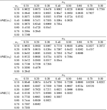
Table 1 shows the ARE ratios for the parameters, b1, b2, andb, respectively.
As expected, our results con…rm that the MLE is asymptotically more e¢ cient than the CLSE for all three parameters, since all the ARE ratios are less than unity. Generally, it is true that more substantial e¢ ciency gains can be obtained from using the ML as the process becomes more persistent (higher values of 1 or 2, or both). Speci…cally, it can be seen from Table 1, Panel 1, that, for a given
value of 2, the ARE of b1 decreases as the value of 1 increases with the largest
advantage for ML occurring when 1 is large and 2 is small. Table 1, Panel 2,
shows that the ARE of b2 is largest when either 1 is large and 2 is small or
1 is small and 2 is large. The third Panel of Table 1 con…rms that substantial
gains are obtained for estimating from persistent processes, especially if either
b1 or b2 approaches unity. But it is interesting to note that, unlike the previous
two cases, the ARE ofb is slightly more sensitive to the scale of 2 and that the
gains are never as large as those available for estimating either of the ’s.
4.3. Monte Carlo Results
In order to compare the relative performance of the estimators in small samples, we carry out Monte Carlo experiments to examine the …nite sample bias and mean squared error (MSE) of alternative estimators6. To achieve this, we generate
ar-ti…cial time series of counts based on the IN AR(2)-P model. As before, values
6We also included the Yule-Walker estimator in the simulations but found its performance
of 1 and 2 as well as their sum, ( 1+ 2), are constrained so that each case
under study is stationary and non-degenerate. The study is based on 1000 repli-cations. For each replication, we estimate the model parameters using alternative estimators and calculate the bias and MSE of parameter estimates. Our simula-tion experiments are performed for sample sizeT = 100 and 500. As in the ARE calculations the qualitative results do not depend on the value of and so we report the = 1 case only.
[Table 2] [Table 3]
The bias results are reported in Tables 2 and 3. It can be seen that, except for a few cases where the ML of b1 is biased up, b1 and b2 are both biased down
andbis biased up. This inverse relationship is to be expected because, for a …xed marginal mean of the seriesXt, decreasing 1 and 2 corresponds to increasing .
The relationship between the bias in b1 and b2, however, is less evident from the
table. But a closer examination of all cases studied, including those unreported, also reveals a negative correlation, despite the fact that both are biased down. This inverse relationship is also expected for similar reason. That is, for a …xed marginal mean of Xt and , a large 1 corresponds to a small 2, and vice versa.
With respect to sample size, Table 3 suggests that the bias of both the CLS and ML estimates is inversely related to the sample size with a minor exception in the case of ^1 for very small values of 1 and 2. Unless the parameters are in the
vicinity of the nonstationary region, the bias of the MLE is less that of CLS for both ^1 and ^2. The MLE of always dominates in terms of bias. These results
hold even at T = 500. This suggests that there is a gain in using the ML over CLS in terms of bias except when close to the nonstationary region.
[Table 4] [Table 5]
The corresponding MSE results are given in Tables 4 and 5. In the case of ^1
Table 4, Panel 1, shows that for small values of 1 the MSE of ML is greater than
that of CLS forT = 100. The corresponding phenomenon holds for ^2 as seen in
5. Conclusion
In this paper, we present a framework for maximum likelihood estimation of GIN AR(p)processes based on a recursive representation of the transition proba-bilities. Using the resulting likelihood, we derive the score function and the Fisher information matrix for the model, which form the basis for conditional maximum likelihood estimation and inference. As in FM, we go on to represent all elements of the Fisher information matrix in terms of timet conditional moments of model components. Using the IN AR(2)-P speci…cation, we investigate the asymptotic gain of implementing the ML method over the commonly used CLS method by calculating the ARE ratio between the two estimators. Our results con…rm that the proposed MLE is asymptotically more e¢ cient than the CLSE and the ef-…ciency gain is most substantial for persistent processes. A Monte Carlo study suggests that there are often small sample gains in terms of bias and MSE to be had.
The proposed maximum likelihood framework also allows for various types of likelihood-based statistical inferences. For instance, given the score functions and elements of the Fisher information matrix, it is possible to test for model adequacy using the information matrix test proposed by McCabe and Leybourne (2000). Moreover, the transition probability function for theIN AR(p)-P process provides a basis for coherent forecasting. These and other issues involved in model selection are examined in Bu and McCabe (2008).
References
Al-Osh M.A. and Alzaid, A.A. (1987) First-order integer valued autoregressive (INAR(1)) process. Journal of Time Series Analysis 8, 261-275.
Alzaid, A.A. and Al-Osh, M.A. (1990) An integer-valued pth-order autoregressive struc-ture (INAR(p)) process. Journal of Applied Probability 27, 314-323.
Azzalini, A. (1983) Maximum likelihood estimation of order m stationary stochastic processes. Biometrika, 70, 381-387.
Bu, R. and McCabe, B.P.M. (2008) Model selection, estimation and forecasting in INAR(p) models: a likelihood based Markov Chain approach. International Journal of Forecasting, 24, 151-162.
Cox D.R. and Hinkley, D. (1974) Theoretical statistics, Chapman and Hall, London.
Davidson, J. (1994) Stochastic limit theory, Oxford University Press.
Dion, J.P., Gauthier, G., and Latour, A. (1995) Branching processes with immigration and integer-valued time series. Serdica,21, 123-136.
Drost, F.C., Van den Akker, R., and Werker, B.J.M. (2008) Local Asymptotic Normal-ity and e¢ cient estimation for INAR(p) models. Journal of Time Series Analysis, Forthcoming.
Du, J. and Li, Y. (1991) The integer-valued autoregressive (INAR(p)) model. Journal of Time Series Analysis 12, 129-142.
Freeland, R.K. (1998) Statistical analysis of discrete time series with applications to the analysis of workers compensation claims data. Ph.D. Thesis, The University of British Columbia, Canada.
Freeland, R.K. and McCabe, B.P.M. (2004) Analysis of low count time series by Poisson autoregression, Journal of Time Series Analysis, 25, 701-722.
Joe, H. (1996) Time series models with univariate margins in the convolution-closed in…nitely divisible class. Journal of Applied Probability 33, 664-677.
Jung, R.C. and Tremayne, A.R. (2006) Coherent forecasting in integer time series mod-els. International Journal of Forecasting, 22, 223-238.
Klimko, L.A. and Nelson, P.I. (1978) On conditional least squares estimation for sto-chastic processes. Annals of Statistics 6, 629-642.
McCabe, B.P.M. and Leybourne, S.J. (2000) A general method of testing for random parameter variation in statistical models in Innovations in Multivariate Statistical Analysis: a Festschrift for Heinz Neudecker, eds. Heijmans, R.D.H, D.S.G. Pollock and A. Satorra, R.D.H, 75-85, Kluwer.
Table 1: Asymptotic Relative E¢ ciency for the IN AR(2)-P Model( = 1)
2
1 0.10 0.20 0.30 0.40 0.50 0.60 0.70 0.80
0.10 0.9622 0.9573 0.9476 0.9362 0.9228 0.9030 0.8680 0.7750 0.20 0.8945 0.9013 0.9051 0.9047 0.8953 0.8635 0.7627
0.30 0.8071 0.8305 0.8531 0.8709 0.8724 0.8182 ARE( 1) 0.40 0.6995 0.7411 0.7885 0.8364 0.8620
0.50 0.5678 0.6240 0.6969 0.7854 0.60 0.4153 0.4728 0.5541
0.70 0.2564 0.2945 0.80 0.1169
2
1 0.10 0.20 0.30 0.40 0.50 0.60 0.70 0.80
0.10 0.9622 0.8933 0.8067 0.7110 0.6088 0.4994 0.3827 0.2572 0.20 0.9579 0.9015 0.8264 0.7397 0.6432 0.5362 0.4157
0.30 0.9452 0.9091 0.8538 0.7853 0.7047 0.6066 ARE( 2) 0.40 0.9122 0.9008 0.8734 0.8370 0.7894
0.50 0.8412 0.8503 0.8517 0.8544 0.60 0.7159 0.7229 0.7205
0.70 0.5300 0.4876 0.80 0.2943
2
1 0.10 0.20 0.30 0.40 0.50 0.60 0.70 0.80
0.10 0.9546 0.9074 0.8479 0.7850 0.7239 0.6668 0.6239 0.6232 0.20 0.9091 0.8507 0.7859 0.7206 0.6607 0.6154 0.6120
0.30 0.8597 0.7923 0.7211 0.6521 0.5966 0.5804 ARE( ) 0.40 0.8135 0.7371 0.6590 0.5898 0.5552
0.50 0.7733 0.6901 0.6092 0.5557 0.60 0.7444 0.6589 0.5921
Appendix A
The following straightforward result is used, often without comment, throughout the proofs. Let X= (X1; : : : ; Xp)0 be a random vector and Y a random variable where X1; : : : ; Xp and Y are mutually independent. Denote their densities as fX(x) and fY(y). Let Z = X01+Y be the convolution of X1 +: : :+Xp; and Y, where1 is a p 1 vector of ones. The conditional moments for (X; Y)given Z are then
E[ (X; Y)jZ]
= E[ (X; Z X01)jZ]
=
R
(x; z x01)fX(x)fY(z x01)dx
fZ(z)
: (14)
We also use the following additional notation. The transition probability den-sity function P(XtjXt 1; : : : ; Xt p)is denoted by
h(XtjXt 1; : : : ; Xt p; 1; : : : ; p; ) =h(XtjX p; )
where X p = (Xt 1; : : : ; Xt p)0, and may be a vector. To simplify integration with respect to a vectors, we sets= (s1; : : : ; sp)0 andd s = (d (s1); ; d (sp))0.
Proof (of Theorem 2.1) We regard Xt as the convolution of 1 Xt 1 and
Y = 2 Xt 2+ + p Xt p+"t, which are by de…nition mutually independent given the pobserved lags. Thus, we can write
h(XtjXt 1; : : : ; Xt p; 1; : : : ; p; )
=
Z
f(s1jXt 1; 1)hY(Xt s1jXt 2; : : : ; Xt p; 2; : : : ; p; )d (s1)
where hY (YjXt 2; : : : ; Xt p; 2; : : : ; p; ) is the conditional probability density function ofY given observations(Xt 2; : : : ; Xt p)and parameters( 2; : : : ; p; ). It is important to note that the quantityhY (YjXt 2; : : : ; Xt p; 2; : : : ; p; )can be evaluated using the expression of the transition probability density function for a GIN AR(p 1) process with parameters ( 2; : : : ; p; ). This is purely a computational device. We thus have the following recursive representation.
h(p)(XtjXt 1; : : : ; Xt p; 1; : : : ; p; )
=
Z
The superscript denotes that the conditional probability density function has the same expression as the transition probability of a GIN AR process with corre-sponding order. The recursion is initialised by
h(1) Xt p 1
X
k=1
sk Xt p; p;
!
=
Z
f(spjXt p; p)g Xt p
X
k=1
sk;
!
d (sp)
which is just the convolution of theGIN AR(1)model with arguments as speci…ed.
Proof (of Theorem 2.2) The conditional log-likelihood function can be written as
lnL( ) = T
X
t=p+1
lnh(XtjX p; )
where
h(XtjX p; ) =
Z "Yp
k=1
f(skjXt k; k)g(Xt p
X
k=1
sk; )
#
d s:
We de…ne
k(s; Xt; ) = p
Y
k=1
f(skjXt k; k)g(Xt p
X
k=1
sk; ):
Hence
h(XtjX p; ) =
Z
k(s; Xt; )d s:
It follows that the corresponding score functions are given by
_
` k = @lnL( ) @ k
= T
X
t=p+1
@
@ kh(XtjX p; )
h(XtjX p; ) ;
_
` = @lnL( )
@ =
T
X
t=p+1
@
@ h(XtjX p; ) h(XtjX p; )
:
Under the conditions of Theorem 2.2 @f(skjXt k; k)
@ k
= (sk;Xt k; k)f(skjXt k; k);
@g("; )
and so
@
@ kh(XtjX p; )
h(XtjX p; ) =
@ @ k
R
k(s; Xt; )d s
h(XtjX p; )
=
R @
@ k [k(s; Xt; )]d s
h(XtjX p; )
=
R
(sk;Xt k; k)k(s; Xt; )d s h(XtjX p; )
= Et[ ( k Xt k;Xt k; k)]:
Note that the last equality follows from the result on conditional expectations in (14). Similarly,
@
@ h(XtjX p; ) h(XtjX p; )
= @ @
R
k(s; Xt; )d s h(XtjX p; )
=
R @
@ [k(s; Xt; )]d s h(XtjX p; )
=
R
Xt p
P
k=1
sk; k(s; Xt; )d s
h(XtjX p; ) = Et[ ("t; )]:
Finally, we have
_ ` k =
T
X
t=p+1
Et[ ( k Xt k;Xt k; k)];
_ ` =
T
X
t=p+1
Et[ ("t; )]:
Proof (of Theorem 2.3) De…ne scalar function k(sk;Xt k; k) and matrix
function ("; ) such that
k(sk;Xt k; k) =
@ (sk;Xt k; k) @ k
;
Under the conditions of Theorem 2.2:
@2f(s
kjXt k; k) @ 2
k
= @[ (sk;Xt k; k)f(skjXt k; k)] @ k
= @ (sk;Xt k; k) @ k
f(skjXt k; k)
+ [ (sk;Xt k; k)]
2
f(skjXt k; k) = k(sk;Xk; k) + [ (sk;Xt k; k)]
2
f(skjXt k; k);
@2g("; )
@ @ 0 =
@[ ("; )g("; )] @ 0
= @ ("; )
@ 0 g("; ) + ("; )
@g("; ) @ 0
= @ ("; )
@ 0 g("; ) + ("; ) ("; )
0 g("; )
= ("; ) + ("; ) ("; )0 g("; ):
It then follows that
@2
@ 2 k
h(XtjX p; )
h(XtjX p; ) =
@2
@ 2 k
R
k(s; Xt; )d s
h(XtjX p; )
=
R @2
@ 2 k
[k(s; Xt; )]d s
h(XtjX p; )
=
R
k(sk;Xt k; k) + [ (sk;Xt k; k)]
2
k(s; Xt; )d s h(XtjX p; )
= Et k( k Xt k;Xt k; k) + [ ( k Xt k;Xt k; k)]2 :
In exactly the same way we can show
@2
@ @ 0h(XtjX p; ) h(XtjX p; )
=Et ("t; ) + ("t; ) ("t; )0 ;
@2
@ k@ h(XtjX p; )
h(XtjX p; )
=Et[ ( k Xt k;Xt k; k) ("t; )];
@2
@ m@ nh(XtjX p; )
Finally, the Fisher information can then be written as follows:
•
` k k = @
2lnL( )
@ 2
k
= T
X
t=p+1
8 < :
@2
@ 2 k
h(XtjX p; )
h(XtjX p; )
" @
@ kh(XtjX p; )
h(XtjX p; )
#29=
;
= T
X
t=p+1
Et k( k Xt k;Xt k; k) + [ ( k Xt k;Xt k; k)]
2
(Et[ ( k Xt k;Xt k; k)])
2
= T
X
t=p+1
fEt[ k( k Xt k;Xt k; k)] +V art[ ( k Xt k;Xt k; k)]g;
•
` m n = @
2lnL( )
@ m@ n
= T
X
t=p+1
( @2
@ m@ nh(XtjX p; )
h(XtjX p; )
@
@ mh(XtjX p; )
h(XtjX p; ) @
@ nh(XtjX p; )
h(XtjX p; )
)
= T
X
t=p+1
fEt[ ( m Xt m;Xt m; m) ( n Xt n;Xt n; n)]
Et[ ( m Xt m;Xt m; m)]Et[ ( n Xt n;Xt n; n)]g
= T
X
t=p+1
Covt[ ( m Xt m;Xt m; m); ( n Xt n;Xt n; n)]:
•
` = @
2lnL( )
@ @ 0
= T
X
t=p+1
( @2
@ @ 0h(XtjX p; ) h(XtjX p; )
@
@ h(XtjX p; ) h(XtjX p; )
@
@ 0h(XtjX p; ) h(XtjX p; )
= T
X
t=p+1
Et ("t; ) + ("t; ) ("t; )0 Et[ ("t; )]Et ("t; )0
= T
X
t=p+1
fEt[ ("t; )] +V art[ ("t; )]g;
•
` k = @
2lnL( )
@ k@
= T
X
t=p+1
( @2
@ k@ h(XtjX p; )
h(XtjX p; )
@
@ kh(XtjX p; )
h(XtjX p; ) @
@ h(XtjX p; ) h(XtjX p; )
)
= T
X
t=p+1
fEt[ ( k Xt k;Xt k; k) ("t; )]
Et[ ( k Xt k;Xt k; k)]Et[ ("t; )]g
= T
X
t=p+1
Covt[ ( k Xt k;Xt k; k); ("t; )]:
Proof (of Theorem 3.3) We sketch the details as the proof follows from a standard Taylor series and remainder argument i.e.
_
` ^ =0= _` ( 0) `• ( 0) ^ 0 +R( )
where 0 is the true value of the parameter and R is a remainder term evaluated
consistency that the scaled remainder term in the Taylor series expansion of the score function is asymptotically negligible using a uniform law of large numbers. Thus the properties of the score determine those of the MLE’s. i.e. scaling and solving we get
T1=2 ^ 0 = T 1`• 1
T 1=2`_ +op(1):
Take an arbitrary linear combination of the score l0`_ . Since the score is the sum of a stationary, ergodic martingale di¤erence sequence (with …nite variance), T 1=2l0`_ automatically satis…es a univariate central limit theorem (see Davidson (1994) p385) and this linear combination is asymptotically normal. Using the Cramer-Wold device the proof is completed by showing that the score has …nite variance and that the information matrix is non-singular. The mapping theorem then delivers the asymptotic distribution of T1=2 ^
0 . These steps are shown
in detail by Freeland (1998) for p= 1 and Bu (2006) for p 1.
Appendix B: Time
t
Conditional Expectations for
IN AR
(
p
)
-P
Process
For the IN AR(p)-P process, the time t conditional expectations are functions of the transition probability. For example, it follows from Theorem 2.1 and the result in (14) that
Et[ 1 Xt 1]
=
min(XXt 1;Xt)
i1=0
i1 Xit11 i11(1 1)Xt 1 i1P(Xt i1jXt 2; : : : ; Xt p)
P(XtjXt 1; : : : ; Xt p)
=
min(XXt 1;Xt)
i1=0
Xt 1 Xit1111 i11(1 1)Xt 1 i1P(Xt i1jXt 2; : : : ; Xt p)
P(XtjXt 1; : : : ; Xt p)
= 1Xt 1
min(XXt 1;Xt)
i1=0
Xt 1 1
i1 1
i1 1
1 (1 1)(Xt 1 1) (i1 1)
P(Xt i1jXt 2; : : : ; Xt p)
1
= 1Xt 1
min(XtX1 1;Xt 1)
i1=0
Xt 1 1
i1
i1
1(1 1)(Xt 1 1) i1
P(Xt 1 i1jXt 2; : : : ; Xt p)
1
P(XtjXt 1; : : : ; Xt p)
= 1Xt 1P(Xt 1jXt 1 1; : : : ; Xt p) P(XtjXt 1; : : : ; Xt p)
:
By applying the same reasoning to (9), the following results hold.
Et[ k Xt k] =
kXt kP(Xt 1jXt 1; : : : ; Xt k 1; : : : ; Xt p) P(XtjXt 1; : : : ; Xt p)
;
Et["t] =
P(Xt 1jXt 1; : : : ; Xt p) P(XtjXt 1; : : : ; Xt p)
;
Et ( k Xt k)2 Et[ k Xt k]
=
2
kXt k(Xt k 1)P(Xt 2jXt 1; : : : ; Xt k 2; : : : ; Xt p) P(XtjXt 1; : : : ; Xt p)
;
fEt["2t] Et["t]g=
2
P(Xt 2jXt 1; : : : ; Xt p) P(XtjXt 1; : : : ; Xt p)
;
fEt[( m Xt m) ( n Xt n)]g
= m nXt mXt nP(Xt 2jXt 1; : : : ; Xt m 1; : : : ; Xt n 1; : : : ; Xt p) P(XtjXt 1; : : : ; Xt p)
;
fEt[( k Xt k)"t]g=
k Xt kP(Xt 2jXt 1; : : : ; Xt k 1; : : : ; Xt p) P(XtjXt 1; : : : ; Xt p)
: