Resource allocation for relay based green communication systems

(1)

Resource Allocation for Relay Based Green

Communication Systems

Thesis submitted in accordance with the requirements of the University of Liverpool for the degree of Doctor in Philosophy

by Linhao Dong

(2)

Declaration

The work in this thesis is based on research carried out at the University of Liverpool. No part of this thesis has been submitted elsewhere for any other degree or qualiﬁcation and it is all my own work unless referenced to the contrary in the text.

(3)

Abstract

The relay based cooperative network is one of the promising techniques for next genera-tion wireless communicagenera-tions, which can help extend the cell coverage and enhance the diversity. To deploy relays eﬃciently with limited power and bandwidth under certain performance requirements, resource allocation (RA) plays an increasingly important role in the system design. In recent years, with the fast growth of the number of mobile phone users, great portion of CO2 emission is contributed by wireless communication

systems. The combination of relay techniques and RA schemes reveals the solution to green communications, which aims to provide high data rate with low power consump-tion. In this thesis, RA is investigated for next generation relay based green wireless systems, including the long-range cellular systems, and the short-range point-to-point (P2P) systems.

In the ﬁrst contribution, an optimal asymmetric resource allocation (ARA) scheme is proposed for the decode-and-forward (DF) dual-hop multi-relay OFDMA cellular systems in the downlink. With this scheme, the time slots for the two hops via each of the relays are designed to be asymmetric, i.e., with K relays in a cell, a total of 2K

time slots may be of diﬀerent durations, which enhances the degree of freedom over the previous work. Also, a destination may be served by multiple relays at the same time to enhance the transmission diversity. Moreover, closed-form results for optimal resource allocation are derived, which require only limited amount of feedback information. Numerical results show that, due to the multi-time and multi-relay diversities, the proposed ARA scheme can provide a much better performance than the scheme with symmetric time allocation, as well as the scheme with asymmetric time allocation for a cell composed of independent single-relay sub-systems, especially when the relays are relatively close to the source. As a result, with the optimal relay location, the system can achieve high throughput in downlink with limited transmit power.

(4)

function of drive power, which gives an easy access to the system level power alloca-tion. To minimise the system total power consumption, the optimal drive power can be allocated to the source node by numerical searching method while satisfying the data rate requirement. The impact of relay locations on the total power consumption is also investigated. It is shown that, with the same data rate requirement, in the small source-relay separation case, DAF consumes slightly less power than DDF; while with larger source-relay separation, DAF consumes much more power than DDF.

(5)

Acknowledgement

Throughout the passing four years, I have received loads of support and help from the following people who generously show their love and encouragement. Without their kindness, this thesis would not have been completed.

I would like to give my deepest gratitude to my supervisor Dr. Xu Zhu, who has been teaching me with great patient and guiding me from a graduate student to a mature researcher. This work no doubt beneﬁts from her invaluable comments. I also appreciate the supervision upon my study from Prof. Yi Huang, who has contributed great comments in some of my publications.

I am grateful to Dr. Sumei Sun at Institute for Infocomm Research (I2R), Singapore, where I spent six months as a postgraduate student attachment. During this period, Dr. Sun gave me lots of advices and guidance in my research work. I would also like to thank Dr. Yeow-Khiang Chia at I2R, who helped me a lot with the information theory. Besides, the following researchers at I2R deserve my gratitude for academical assistance and family-like atmosphere, and they are Dr. Koichi Adachi, Dr. Lin Shan, Dr. Xiaojuan Zhang, Mr. Gang Yang, Dr. Jingon Joung, Dr. Peng-Hui Tan, and Dr. Chi-Keong Ho. It is my pleasure to share this good time with you.

I would like to thank my (previous) colleagues in the Wireless Communication and Smart Grid group: Dr. Nan Zhou and Dr. Jingbo Gao for inspiring discussions in resource allocation schemes, Mr. Yufei Jiang for sharing views in the channel estimation theory, Mr. Teng Ma for the tutorials in channel measurement and body ﬁtness, Mr. Chao Zhang and Yanghao Wang for discussions in smart grid and photography, Mr. Wenfei Zhu, Mr. Chaowei Liu, Mr. Jun Yin, Mr. Qinyuan Qian, and Mr. Yang Li for sharing a family-like atmosphere and delicious meals. I am so pleased to see this group now is growing up with the extra three new students: Mr. Mohammad Heggo, Mr. Kainan Zhu, and Mr. Zhongxiang Wei. Your guys are the ﬁnest!

I would also like to show my great appreciation to the Chinese congregations in Liverpool and Singapore of Jehovah’s Witnesses. Thanks to your Christian love and spiritual support, I could get over the loneliness and ﬁnd the meaning of real life.

Finally, my gratitude is dedicated to my parents. Without their support and love, I would have no opportunity to study abroad and pursue this degree.

(6)

Chris-tine Hobden and Mrs. Coi-Wan Tam. You are the true worriers ﬁghting against cancer. To God YHWH

(7)

List of Figures

2.1 The propagation of the EM wave as a closed sphere surrounding the

transmitter, (d– the distance between Tx and Rx) . . . 4

2.2 An simpliﬁed example of multipath eﬀect of EM wave . . . 6

2.3 The received signals via diﬀerent paths . . . 7

2.4 Fading types classiﬁed by symbol period . . . 9

2.5 Block diagram of a communication system . . . 10

2.6 Binary symmetric channel . . . 12

2.7 Simpliﬁed block diagram of the OFDM system . . . 18

2.8 Block diagram of an OFDMA system in downlink . . . 20

2.9 A three-terminal relay network . . . 21

3.1 Illustration of the relationship between a passband spectrum and its baseband equivalent . . . 28

3.2 The ampliﬁcation model of PA . . . 29

3.3 Illustration of the division of channels in a multi-carrier system, where f represents the frequency , and the red portions are guard bands . . . 30

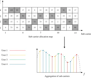
3.4 An example of sub-carrier allocation, where the numbers in the cube are the relative values of SNR, and the grey parts indicate the maximum SNR amongst users . . . 31

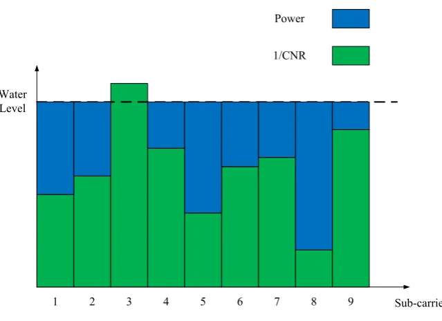
3.5 Illustration of the water-ﬁlling algorithm . . . 33

4.1 A multi-relay based OFDMA cellular system . . . 35

4.2 Impact of distance between the source and the mid circle of relays on maximum achievable throughput, withK= 4 relays and L= 8 destina-tions . . . 47

4.3 Impact of the number of relays on maximum achievable throughput, with L= 16 destinations . . . 48

4.4 Impact of the number of destinations on maximum achievable through-put, with K= 4 relays . . . 48

(11)

5.1 Illustration of a three-terminal DxF relay network . . . 53 5.2 The simpliﬁed block diagram of an DAF relaying . . . 54 5.3 The simpliﬁed block diagram of DDF relay node, where the source and

destination are omitted due to same structures with DAF . . . 56 5.4 Illustration of a message node and its decoding neighbours, whereζ = 3

and the total number of iterations is 3 . . . 58 5.5 The impact of dive power on the total power consumption in DAF

re-laying, wheredSD=dSR=dRD = 6 m . . . 64 5.6 The impact of dive power on the total power consumption in DDF

re-laying, wheredSD=dSR=dRD = 6 m . . . 64 5.7 The impact of drive power on the total decoding power in DDF relaying 65 5.8 The impact of drive power on total PA power in DDF relaying . . . 66 5.9 The impact of the distances between each nodes on the power

consump-tion, where dSR = dRD = dSD/ √

2. Solid lines: DDF; dashed lines: DAF . . . 66 5.10 The impact of relay’s location on the power consumption, where dSD =

7.07 m. Solid lines: DDF; dashed lines: DAF . . . 67

(12)

List of Tables

2.1 PL exponent values in diﬀerent scenarios . . . 6 2.2 Types of multipath fading . . . 8 2.3 Types of relaying protocols . . . 24

4.1 The parameter setup in the multi-relay based OFDMA cellular system . 46

5.1 The parameter setup in the relay based short-range communication systems 63

A.1 Time line of evolution of mobile telephony standards . . . 72

(13)

Nomenclature

3G third generation

3GPP third generation partnership project

4G fourth generation

5G ﬁfth generation

AD analogue-to-digital

AF amplify-and-forward

AMPS advanced mobile phone system

ARA asymmetric resource allocation

AWGN additive white Gaussian noise

BEP bit error probability

BER bit error rate

BS base station

BSC binary symmetric channel

CDMA code-division multiple access

CEPT European Conference of Postal and Telecommunications Administrations

CIR channel impulse response

CNR channel-to-noise ratio

CP cyclic preﬁx

CSI channel state information

CoMP coordinated multipoint

(14)

DDF diversity decode-and-forward

DF decode-and-forward

DxF diversity x forward

EM electromagnetic

ERP eﬀective radiated power

EV-DO evolution-data optimized

FDMA frequency-division multiple access

FFT fast Fourier transform

GSM global system for mobile communications

HSPA high speed packet access

ICI inter-carrier interference

IFFT inverse fast Fourier transform

ISI inter-symbol interference

ITU International Telecommunication Union

IxF intersymbol interference x forward

KKT Karush-Kuhn-Tucker

KL Kullback-Leibler

LNA low noise ampliﬁer

LOS line-of-sight

LS least square

LTE long term evolution

MAC medium access control

MIMO multiple-input and multiple-output

MMSE minimum mean squared error

MRC maximum ratio combining

(15)

MxF multi-hop x forward

OFDM orthogonal frequency-division multiplexing

OFDMA orthogonal frequency-division multiple access

P2P point-to-point

PA power ampliﬁer

PAE power added eﬃciency

PAPR peak-to-average power ratio

PE processor element

PL path loss

QoS quality of service

RA resource allocation

RF radio frequency

RMS root-mean-square

SA sub-carrier allocation

SCxF split-combine x forward

SNR signal-to-noise ratio

SRA symmetric resource allocation

TDMA time-division multiple access

UMTS universal mobile telecommunications system

VLSI very-large-scale integration

WiMAX worldwide interoperability for microwave access

WLAN wireless local area networks

WPAN wireless personal area networks

(16)

Chapter 1

Introduction

1.1 Motivation

Wireless communications have experienced a rapid development over the past decades [2] [3], and a surge of research activities have been carried out to provide a higher system capacity [4], a better quality of service (QoS) [5], lower power consumption [6], and more ﬂexible system coverage [7]. However, according to a recent survey, 2% of the global CO2 emission is contributed by the information and communication technology

[8], and this ﬁgure is expected to increase each year. To provide the high data rate with low power consumption, the concept of ‘green communications’ attracts much attention [9].

(17)

1.2 Research Contributions

This thesis ﬁrst presents a joint ARA scheme for relay based long-range communication systems, where the RA consists of power allocation, sub-carrier allocation, and time duration allocation. By applying this RA scheme, the system throughput is maximised with limited transmit power, leading to a high energy eﬃciency. After that, a system power consumption model is proposed for relay based short-range green communication systems at 60 GHz, where the transmit power, PA power, and decoding power are considered as functions of the drive power of PA. By numerically searching method, the optimal drive power can be allocated at the source node to minimise the system power consumption while satisfying the data rate requirement.

The research during this PhD study has produced the following main contributions:

• An ARA scheme for DF dual-hop multi-relay OFDMA systems for long-range communication is proposed. This work is diﬀerent in the following aspects. First, this is the ﬁrst work to apply asymmetric time allocation to a general multi-relay multi-destination system. As a result, it enhances the degree of freedom for transmission over the previous symmetric RA (SRA) scheme. Second, an optimal algorithm is proposed to perform joint time, power and subcarrier allocation to obtain the global optimal results, with only limited amount of feedback informa-tion from relays and destinainforma-tions. Compared to [20], the proposed work allows multiple relays to serve a single destination by using CoMP technique, which enhances the degrees of freedom. Numerical results show that, thanks to the multi-time and multi-relay diversities, the proposed ARA scheme outperforms the SRA algorithm in [21], as well as the ARA algorithm in [20], with higher achievable system throughput, especially when the relays are relatively close to the source. Moreover, impact of the relays’ locations on the results of asymmetric time allocation is demonstrated.

(18)

on the system performance is also investigated, and the comparison between the DAF and DDF relaying is made.

1.3 Thesis Organisation

The rest of this thesis is organised as follows. The wireless channels and systems are introduced in Chapter 2. Chapter 3 presents the literature survey on RA of broadband wireless communication systems. An ARA scheme for relay based long-range cellular systems is proposed in Chapter 4, where both optimal and suboptimal algorithms are considered. In Chapter 5, a power consumption model with its power allocation scheme is proposed for 60 GHz relay based short-range P2P communications, where the DAF and DDF relaying strategies are compared. Conclusions and future work are presented in the ﬁnal chapter.

1.4 Publication List

A number of publications during the study of this research are listed below, which partially contribute to the thesis.

1. L. Dong, X. Zhu, Y. Jiang and Y. Huang “Optimal Asymmetric Resource Al-location for Dual-Hop Multi-Relay Based Downlink OFDMA Systems,” Mobile Computing, vol. 2, no. 1, pp 1-8, Feb. 2013.

2. L. Dong, S. Sun, X. Zhu, and Y.-K. Chia, “Power Eﬃcient 60 GHz Wireless Com-munication in Cooperative Networks,” submitted toIEEE Trans. Veh. Technol. 3. L. Dong, X. Zhu, N. Zhou, and Y. Huang, “Asymmetric Resource Allocation for Decode-and-Forward Multi-Relay Systems,” inProc. IEEE WiCOM’11, Wuhan, China, Sep. 2011.

4. L. Dong, X. Zhu, and Y. Huang, “Optimal Asymmetric Resource Allocation for Multi-Relay Based LTE-Advanced Systems,” in Proc. IEEE GLOBECOM’11, Houston, USA, Dec. 2011.

5. L. Dong, X. Zhu, and Y. Huang, “Optimal Asymmetric Resource Allocation for Dual-Hop Multi-Relay LTE-Advanced Systems in the Downlink,” inProc. IEEE ICC’13, Budapest, Hungary, Jun. 2013.

(19)

Chapter 2

Research Overview

In this chapter, the wireless communication channel models and the channel capacity are described in Section 2.1 and 2.2, respectively. An overview of wireless communica-tion systems is presented in Seccommunica-tion 2.3. In Seccommunica-tions 2.4 and 2.5, the fundamentals of OFDM and relay techniques are introduced.

2.1 Wireless Communication Channel Models

The wireless channel is the air interface that links the transmitter and the receiver. Its properties dominate the information-theoretical capacity of communications, the performance limit of wireless systems, and the QoS level. Hence, it is essential to know the behaviour of wireless channels, which helps in the system design.

2.1.1 Large-Scale Path Loss

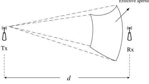
In the propagation of the electromagnetic (EM) wave through a certain medium, the energy of the carried signals is radiated out from a transmitter. If the receiver can ‘pick

d

Tx _Rx

[image:19.595.201.445.531.668.2]

Effective aperture

(20)

up’ part of this energy, it is possible that the information contained in the signals can be detected at the receiver, thus a data link is established.

If the radiation pattern of the antenna is assumed as isotropic, and the medium is as a vacuum environment, the EM wave propagates in a pattern of a sphere as shown in Fig. 2.1, where ‘Tx’ denotes the transmitter and ‘Rx’ denotes the receiver. The energy conservation law tells that the total energy of signals remains unchanged surrounding the closed free space of the transmitter. With the increasing of the distance that the EM wave travels, the total surface area of the sphere also grows correspondingly, which causes the reduction of the power at the unit area. As a result, the strength of the signals is attenuated. The concept of ‘power’ is used instead of ‘energy’ without the loss of generality. dis defined as the distance between Tx and Rx,PT as the wavelength of the EM wave, andGT as the gain of the transmitter antenna. The power density, or effective radiated power (ERP) [2], can be defined as

Pef f =

GTPT

4πd2 (2.1)

From (2.1), it can be observed that if the distancedis doubled, the ERP will decrease by around 6 dB.

At the Rx,GRis defined as the antenna gain of the receiver. The effective aperture [23] can be simplified as

aef f =

λ2

4πGR (2.2)

where λis the wavelength of the EM wave at central frequency fc. According to the Frii’s equation [2], the received power can be written as

PR=Pef f ×aef f =PTGTGR

( λ 4π )2( 1 d )2 (2.3)

Thus, the free-space path loss (PL) [24] is expressed as

Af ree(d) =

PR

PT

=GTGR

( λ 4π )2( 1 d )2 (2.4)

Ifα is deﬁned as the PL exponent, a general expression of PL can be written as

A(d) = PR

PT

=GTGR

( λ 4π )2( 1 d )α (2.5)

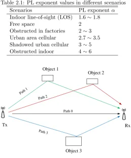
The value of α can be ﬁtted by a huge number of measurements, and some example values of PL exponent are shown in Table 2.1.

In the practical usage, PL is usually given in the log form [25]. Therefore, (2.5) can be rewritten as

AdB(d) =A0+ 10αlog10d (2.6)

whereA0 = 10 log10 (4π)2

GTGRλ2. Due to the fact that PL is mainly aﬀected by the distance,

(21)

[image:21.595.195.454.81.394.2]

Table 2.1: PL exponent values in diﬀerent scenarios

Scenarios PL exponentα

Indoor line-of-sight (LOS) 1.6∼1.8

Free space 2

Obstructed in factories 2∼3 Urban area cellular 2.7∼3.5 Shadowed urban cellular 3∼5 Obstructed indoor 4∼6

Tx Rx

Object 3 Object 1

Object 2

Path 0

Path 1

Path 2

Path 3

Figure 2.2: An simpliﬁed example of multipath eﬀect of EM wave

2.1.2 Small-Scale Multipath Fading

Multipath fading is the rapid fluctuation of channel gain and change of phases over a short period of time or distance, which causes rapid small-scale variation of signals. In the urban area, the transmitted EM wave could be reflected, diffracted and scattered by objects such as buildings, vehicles, trees, and rough surfaces. Hence, the signal travels via different paths to the receiver. Fig. 2.2 shows the simplified model of the multipath effect, where path 0 indicates the LOS path. Each of the paths generates a unique wave of transmitted signal with the randomly distributed amplitude, phase, and delay. As a result, all these EM waves are combined at the receiver (as shown in Fig. 2.3), which causes the signal distortion and fading.

2.1.2.1 Parameters of Multipath Fading

Defining gi and τi as the channel gain and delay for ith path, respectively, the mean excess delay [24] is the first moment of the power delay profile, and can be defined as ¯

τ =∑_i|gi|2τi/

∑

(22)

0 1 2 3

Amplitude

Path 0

Path 1

Path 2

Path 3

Figure 2.3: The received signals via diﬀerent paths

central moment of the power delay proﬁle, which can be deﬁned as

µ=

√

τ¯2₋_(¯_τ₎2 _(2.7)

where τ¯2 = ∑_i|gi|2τi2/

∑

i|gi|2. The RMS delay spread indicates the eﬀect of multi-path. In other words, the higher the RMS delay spread is, the larger the eﬀect will be.

In wireless communications, coherence bandwidth Bc is deﬁned as the range of frequencies where two frequency components have a strong potential correlation for amplitude [3]. For instance, if 95% coherence bandwidth is 5 kHz, the behaviours of two frequency components, which are 5 kHz or less separated apart, are nearly the same. Roughly, coherence bandwidth can be approximated from RMS delay spreadµ, i.e.,Bc,50%≈1/5µ,Bc,90% ≈1/50µ.

When the mobile user moves with a relative velocity v with the base station as the inertial frame of reference, there is a shift on the frequency of signals. This effect is called Doppler effect [24], following the name of the Austrian physicist Christian Doppler. Definingθ as the angle between the direction of the received signal wave and the direction of the mobile user’s motion, the Doppler shiftfd can be expressed as

fd=

v

λcosθ (2.8)

When θ= 0, the direction of the received signal is in accordance with the direction of motion, where Doppler shift achieves the maximum asfd max=v/λ.

(23)

2.1.2.2 Types of Multipath Fading

Since the characteristics of the signal wave and channel are defined, the different types of small-scale multipath fading can be categorised by some thresholds. If Ts and Bsg are defined as the symbol period and signal bandwidth, respectively, there are four different types of multipath fading shown in Table 2.2.

Table 2.2: Types of multipath fading Flat fading Bsg < Bc,50%,Ts>5µ Frequency selective fading Bsg > Bc,50%,Ts<5µ Slow fading Ts≪Tc

Fast fading Ts> Tc

These types of fading are explained in the following details:

• Flat fading: When the symbol period is longer than the RMS delay spread (i.e.,

Ts > 5µ), or the bandwidth of the transmitted signal is less than the channel coherence bandwidth (i.e., Bsg < Bc,50%), all the frequency components within

the transmitted bandwidth have nearly the same channel gain and linear phase. In this scenario, the channel is referred to as flat fading. Flat fading is the most common type described in the literature. The channel gains of flat fading vary in time randomly, and they follow different distributions such as Rayleigh fading, Rician fading, and Nakagami fading [2].

• Frequency selective fading: When the symbol period is shorter than the RMS delay spread of a wireless channel (i.e.,Ts<5µ), or the bandwidth of the trans-mitted signal is larger than the channel coherence bandwidth (i.e.,Bsg > Bc,50%),

previous transmitted symbols could easily cause interference to current transmit-ted symbols. This interference is called inter-symbol interference (ISI). In the frequency domain, the ISI is presented by a formation that frequency compo-nents of the received signal’s spectrum undergo diﬀerent amplitudes. Hence, this fading is referred to as frequency selective fading.

• Slow fading: The channel remains unchanged over one or several symbol periods is called slow fading channel, where the symbol period is much less than the coherence time (i.e.,Ts≪Tc).

• Fast fading: In this scenario, the channel changes so fast that the signal passes through diﬀerent channels even within one symbol period. In other words, the symbol period is longer than the coherence time (i.e.,Ts> Tc).

(24)

s

T

s

T

c

T 5

Flat slow fading Flat fast fading

Frequency selective slow fading

Frequency selective fast fading

Figure 2.4: Fading types classiﬁed by symbol period

fading channel, and frequency selective fast fading channel. Fig. 2.4 illustrates the four multipath fading combinations with RMS delay spread and coherence time as thresholds. Although there are no clear boundaries amongst these types, the channel is still assumed as ‘pure’ ﬂat slow fading or ‘pure’ frequency selective fast fading, etc. Throughout this thesis, frequency selective slow fading channels are focused on.

2.1.3 Fading Channel Model

In this subsection, the fading channel model is introduced. For a wireless communica-tion system, each symbol is transmitted from the transmitter within signal bandwidth

Bsg, and during symbol period Ts. Assuming there are Np paths between the trans-mitter and receiver, the channel impulse response (CIR) can be written as

g(t) = N∑p−1

i=0

giδ(t−τi) (2.9)

where δ(·) is defined as the impulse function. Note that when Np = 1, the channel is classified as flat fading.

It is assumed that each path is independent from another with diﬀerent delays, and

gi is an independent zero mean complex Gaussian random variable. The variance ofgi follows the discrete exponential power delay proﬁle as

E{|gi|2

}

=b·exp

(

−τi

µ )

(2.10)

where b is the normalising factor. Usually, |gi| follows the Rayleigh distribution, of which the probability density function can be written as

p(|gi|) = |

gi|

V2 exp (

−|gi|2 2V2

)

(25)

Source Encoder Channel Decoder Destination Noise Source

X Y

Figure 2.5: Block diagram of a communication system

where V is the RMS voltage of the received signal, and V2 denotes the time average power of the received signal.

Letting f(t) represent the pulse shape with the eﬀects of the transmit and receive ﬁlters, the overall CIR is the convolution of the physical CIRg(t) withf(t), as

h(t) =f(t)∗ N∑p−1

i=0

giδ(t−τi) = N∑p−1

i=0

gif(t−τi) (2.12)

In the simulation of a wireless system, the raised-cosine filter, which is an implemen-tation of a low-pass Nyquist filter, is widely applied to approximate the filter effect at transmitter and receiver [26]. Defining φas the roll-off factor,f(t) can be written as

f(t) = sinc

( t Ts

)_cos(πφt Ts

)

1−4φ_T22t2 s

(2.13)

whereTs is the symbol period.

2.2 Channel Capacity

In the information theory, channel capacity of a communication channel is the tightest upper bound on the data rate that can be reliably transmitted [27]. As early as in 1948, Claude E. Shannon derived this upper bound for both discrete and continuous channels [28], which is called Shannon capacity nowadays. According to his results, capacity of a channel is given by the supremum of the average mutual information between the source and destination.

Now consider a simplest channel model as shown in Fig. 2.5, where X and Y are discrete random variable ensembles representing the input and output of the channel, respectively. pX|Y(x|y) is deﬁned as the conditional probability density function ofX givenY, which is determined by the channel. DeﬁningpY(y) as the marginal probability density ofY, and pX,Y(x, y) as the joint probability density, where

(26)

deﬁned as

I_X_|_Y(x|y) =−logp_X_|_Y(x|y) (2.15) Letting pX(x) denote the marginal probability density ofX, the self-information of x can be written as

IX(x) =−logpX(x) (2.16) Hence, the mutual information between X and Y can be written as the diﬀerence between (2.15) and (2.16), which is

IX;Y(x, y) =IX(x)−IX|Y(x|y) = log

p_X_|_Y(x|y)

pX(x)

(2.17)

From [29] it is known that the entropy is a measure of the uncertainty in random variable ensembles, and can be calculated as the expected value of self-information.

H(X|Y) is deﬁned as the conditional entropy ofXover joint XY ensemble, and it can be expressed as

H(X|Y) =− ∑ x∈X,y∈Y

pX,Y(x, y) logpX|Y(x|y) (2.18)

Similarly, the entropy ofX can be written as

H(X) =−∑ x∈X

pX(x) logpX(x) (2.19)

The average mutual information can be written as

I(X;Y) =H(X)−H(X|Y)

= ∑

x∈X

∑

y∈Y

pX,Y(x, y) log

pX|Y(x|y)

pX(x)

= ∑

x∈X

∑

y∈Y

pX,Y(x, y) log

pX,Y(x, y)

pX(x)pY(y)

(2.20)

If variablesX and Y are continuous, (2.20) can be rewritten as

I(X;Y) =

∫

X

∫

Y

pX,Y(x, y) log

pX,Y(x, y)

pX(x)pY(y)

dxdy (2.21)

When the ensembles X and Y are mutually independent, the joint probability density can be written aspX,Y(x, y) =pX(x)pY(y). As a result, (2.17) and (2.21) both become zero. This case indicates that if the channel quality is extremely low, it is impossible to transmit any information from the source to destination. In other words, mutual information describes how much information can be shared between two communication nodes. The channel capacity thus can be deﬁned as

C = sup pX(x)

I(X;Y) (2.22)

(27)

0 0

1 1

p

1 p

Source Destination

Figure 2.6: Binary symmetric channel

2.2.1 Binary Symmetric Channel

Since digital systems are most widely applied in communication network, the messages transmitted between the source and destination can be simply regarded as binary se-quences composed by ‘0’ and ‘1’. To describe the behaviour of the transmission, BSC model is introduced [29].

Fig. 2.6 illustrates the basic principle of BSC, where p is the ﬂipping probability of binary symbol. When the source transmits only binary symbols, the destination can receive either 0 or 1. If the channel output is observed from the destination, the ﬂipping probability can be expressed as

pX|Y(x= 0|y= 0) =pX|Y(x= 1|y= 1) = 1−p (2.23)

pX|Y(x= 1|y= 0) =pX|Y(x= 0|y= 1) =p (2.24)

The entropyH(X) of ensembleX is a binary entropy function [27], as

H(X) =−∑ X

pX(x) log2pX(x)

=−plog₂p−(1−p) log₂(1−p)

(2.25)

The capacity can be written as

C = 1−H(X) (2.26)

For instance, if the ﬂipping probability isp= 0.01, the capacity isC ≈0.92.

The idea of BSC is simple. While in the system design, the expression of BSC capacity is not practical since ﬂipping probability cannot reveal much information about parameters setup, such as transmit power, bandwidth, etc. in the system. Therefore, a more practical form of channel capacity is in need.

2.2.2 Additive White Gaussian Noise Channel

(28)

the particles contained in electronic components, black body radiation from the earth, and celestial sources, etc. The noise amplitude follows the Gaussian distribution, thus this kind of noise is namedGaussian noise [24].

In the measurement and research, Johnson-Nyquist noise [3] is usually approximated as AWGN. DeﬁningT as the temperature in Kelvin, the single-sided noise power spec-tral densityN0 can be deﬁned as

N0=kBT (2.27)

where kB as the Boltzmann’s constant, of which the value is 1.38×10−23 J/K. B is deﬁned as the bandwidth of the noise, the noise power σ2

0 thus can be written as σ₀2=BN0. Deﬁning z(z∈Z) as the AWGN noise, the probability density ofz can be

expressed as

pZ(z) = √ 1 2πσ0

exp

(

−|z|2 2σ2 0

)

(2.28)

Now consider a transmission where the source transmits the symbol x (x ∈ X, and E{|x|2} = 1) with the average power PT over distance dbetween the source and destination. The noise z is added to the received symbols. At the destination, the received symbol y (y∈Y) can be expressed as

y=√A(d)PTx+z (2.29) whereA(d) is the PL. From [28], the entropy of the noise Z is

H(Z) =−

∫

Z

pZ(z) logpZ(z)dz

= 1

2log 2πeσ

2 0

(2.30)

It is assumed that the transmitted symbol ensemble X is independent from noise Z. Hence, the average power ofY can be written as

E{|y|2}=E

{

|√A(d)PTx+z|2

}

=A(d)PT +σ02

(2.31)

Since y =√A(d)PTx+z, Y can be regarded as the variable which follows Gaussian distribution with varianceA(d)PT +σ02. As a result, the entropy H(Y) can be written

as

H(Y) = 1

2log 2πe

(

A(d)PT +σ20 )

(2.32)

In [28], Shannon proved that the mutual information I(X;Y) for AWGN channel can be expressed as

I(X;Y) =H(X)−H(X|Y) =H(Y)−H(Z) (2.33) As a result, substituting (2.30) and (2.32) into (2.33), the capacity for AWGN channel can be approximated as

C= 1 2log

(

1 +A(d)PT

σ2 0

)

(29)

Note that if the modulation is complex, there is no pre-log factor 1/2.

Now consider a complex modulation in the continuous-time AWGN channel with bandwidth B Hz. By the passband-baseband conversion [24], there should be at least

B complex samples in one second. Hence, the channel capacity can be written as

C=Blog

(

1 +A(d)PT

BN0 )

, bit/s (2.35)

where the received SNR is A(d)PT/BN0. Equation (2.34) and (2.35) with their

alter-native forms are frequently quoted throughout this thesis.

2.2.3 Fading Channel

In this scenario, it can be assumed that the complex channelhshas the same amplitude for all the frequency components within channel state s (s∈ S), where the expected value over all the states isE{|hs|2}=A(d). Cs is deﬁned as the channel capacity ofhs, and p(s) as the probability that the channel remains state s over all the time period. The channel capacity for fading channel can be expressed as [30]

C=∑

S

Csp(s) (2.36)

Deﬁningx[n] as the transmitted symbol at discrete timen, and 1/Bas the sample rate, the instantaneous symbol at receiver can be written as

y[n] =hs[n]√PTx[n] +z[n] (2.37) where PT is the transmit power, and z[n] is the sampled AWGN noise. The instan-taneous channel-to-noise ratio (CNR) at receiver is deﬁned asγ[n] =|hs[n]|2/BN0, of

which the expected value isγ =A(d)/BN0. Lettingpγ(γ[n]) =p(γ[n] =γ) denote the

probability distribution, (2.36) can be rewritten as

C=

∫

γ

Blog (1 +PTγ[n])pγ(γ[n])dγ[n] (2.38)

where the channel state set S is assumed continuous. According to Jensen’s equal-ity, ES{CS(γ[n])} ≤ CS(ES{γ[n]}) always holds [2], which shows the fading channel capacity is no larger than the AWGN capacity with the same average transmit power. If the receiver can give the feedback of the full channel state information (CSI), it is possible to adjust the transmit power PT(γ[n]) at the source with γ[n]. Thus, the channel capacity becomes

C = max PT(γ[n])

∫

γ

Blog (1 +PT(γ[n])γ[n])pγ(γ[n])dγ[n] (2.39)

subject to:

PT(γ[n])≤PT (2.40)

(30)

2.3 Overview of Wireless Communication Systems

Nowadays, wireless communication is so common that it enables people to get internet access anywhere with mobile devices. However, the radio transmission has a long his-tory of development. When the days back to 1860s, it was mathematically and experi-mentally proved by James Clerk Maxwell that EM waves have the ability of propagating in a certain medium [31]. After more than ten years of early attempts with inventions, in 1879 David Edward Hughes discovered that sparks would excite signals that can be detected in a telephone receiver, and he demonstrated the transmission of Mores code with his invention called ‘spark-gap transmitter’ [32]. In the late 1880s, Heinrich Rudolf Hertz observed sparks can be transformed back from electric waves by a slotted metallic circle (like a loop antenna) from a modified spark-gap transmitter, which is the first time of wireless transmission throughout history [33]. Around 1893, Nikola Tesla suggested the information could be transmitted without wires, and proposed that the radiation property in radio frequency wave might be utilised in telecommunication. In 1897, Guglielmo Marconi established the ‘Wireless Telegraph Trading Signal Com-pany’, and built a radio station at Isle of Wright to start the experimental usage of wireless transmission. Following his series of demonstrations on the radio transmission at different places, the commercialisation of radio was motivated.

After a few pioneering attempts since 1918, the first commercialised mobile tele-phone service (MTS) was commenced by AT&T in 1948, which provided services for 5,000 customers [34]. In the late 1960s, the early model of modern cellular network was proposed by Richard H. Frenkiel [35], which includes the basic idea of frequency reuse and handoff. Since then, the cellular network architecture has been regarded as the standard structure of multiuser wireless communication networks. The first cellular network was deployed in North America around 1978, which is called advanced mo-bile phone system (AMPS). In this system, frequency-division multiple access (FDMA) scheme is accepted as a solution to spectrum sharing. However, due to the disadvantage of the unencrypted analogue signals, the voice messages were easily scanned. With the revolution of the semiconductor and very-large-scale integration (VLSI) technologies, the wireless technology stepped into the digital age in the early 1990s. The first second generation (2G) standard network, global system for mobile communications (GSM) system, was launched in 1991 in Finland. Until 2007, GSM had provided its service to over 2 billion customers around the world [36].

(31)

from customers for the data services. Hence, to meet this data rate requirement, evolution-data optimized (EV-DO) [39] and high speed packet access (HSPA) [40], which are regarded as 3.5G standards, were launched in 2003 and 2005, respectively. The maximum download speeds for HSPA and EV-DO are 14.4 Mbit/s and 4.9×N

Mbit/s, respectively, and their maximum upload speeds are 5.76 Mbit/s and 1.9×N

Mbit/s, respectively, where N is the number of 1.25 MHz spectrum chunk used in EV-DO systems. The updated version of HSPA, which is called as HSPA+ [41], was proposed to improve the system capacity of the early version. The downlink and uplink peak data rates of HSPA+ are 42×N and 11×N, respectively, whereN is the number of 5 MHz carriers employed.

Recently, the markets in North America, Asia and Europe have launched the 3.9G standards, worldwide interoperability for microwave access (WiMax) and long term evolution (LTE) systems. Based on the IEEE 802.16 protocol, WiMAX can provide broadband access with downlink and uplink speeds up to 75 Mbit/s and 25 Mbit/s, respectively. Meanwhile, the current LTE, which belongs to 3rd generation partnership project (3GPP) release 8, oﬀers up to 326.4 Mbit/s and 86.4 Mbit/s as the peak down-link and updown-link data rates. After 30 years of development from 1G, it is so surprising to see that the data rate of LTE is 5,800 times of the peak data rate of AMPS in downlink (the peak data rate of AMPS is 56 kbit/s)! While, the pursuing of higher data rate in wireless communication never stops. Developed from WiMAX and LTE, WiMAX 2 and LTE-Advanced were proposed in 2011 as the 4G standards to support peak downlink data rate up to 1 Gbit/s and peak uplink data rate up to 500 Mbit/s [42]. In LTE-Advanced systems, relay and coordinated multipoint (CoMP) techniques are adopted to help improve the cell-edge performance [12] [43]. How about the 5G network? It is believed that millimetre-wave communication is one of the promising solutions to the future 5G standard [44] [45], while there are still many issues need to be addressed. Chapter 5 introduces some technical details about power consumption of millimeter-wave communication systems. All the aforementioned wireless communica-tion techniques are summarised in Table A.1 of Appendix A. As shown in the table, it can be observed that in the early days of wireless communication, each country had her own standards. While with the tendency of globalisation, the boundaries of standards between countries have been merging.

2.4 OFDM Techniques

(32)

and acceptable resolution of images. While, the higher the transmit data rate, the larger the impact of frequency selective fading is, which prevents the system satisfying the QoS of online video.

One of the existing solutions is deploying high speed Wi-Fi access points to provide internet connection at the local area. This communication protocol is based on the IEEE 802.11 series. In 1999, 802.11a (now is specified as clause 18 [46]) was proposed to use orthogonal frequency-division multiplexing (OFDM) as the modulation scheme to combat with the impact of frequency selective fading. Since then, OFDM has been effectively applied in the successive protocols such as 802.11g/n, and the peak down-link data rate can achieve up to 150 Mbit/s for one stream [46]. Compared to other techniques such as time-division multiple access (TDMA) and CDMA, OFDM requires less complex equalisation filters, has higher spectral efficiency, and is robust against the ISI. However, some disadvantages of OFDM limit the system performance in some particular situations. One is that OFDM signals have high peak-to-average power ratio (PAPR), which causes poor power efficiency by applying linear amplification circuity at transmitter [47]. The solutions of PAPR problem are discussed in Section 3.1. An-other is that OFDM signal transmission is sensitive to Doppler shift [26], which causes inter-carrier interference (ICI). A variety of schemes are proposed in [48] [49] [50] to cancel the ICI. Hence, OFDM has been selected as one of the key techniques in 4G standard, such as LTE-Advanced [51], after weighting the pros and cons.

2.4.1 OFDM

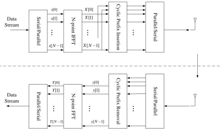
OFDM uses a large number of closely-spaced orthogonal sub-carriers to carry data [52]. The data is reformed into several parallel streams, with each stream on one sub-carrier. Then each sub-carrier is modulated with a conventional modulation scheme at a low symbol rate, maintaining total data rates similar to conventional single-carrier modulation schemes in the same bandwidth. The OFDM streams can be viewed as many slowly-modulated narrow-band signals rather than one rapidly-modulated wide-band signal, which allows low-complex equalisation design.

Fig. 2.7 shows the basic structure of OFDM in a communication system, where

x[n] (n = 0, ..., N −1) are the source symbols, and N is the number of sub-carriers. The cyclic prefix (CP) is designed to eliminate the multipath effect when the OFDM symbols arrive at the receiver. Defining Ts as the symbol period, the transmitted symbols after the inverse fast Fourier transform (IFFT) can be expressed as

X(t) = 1

N

N_∑−1

i=0

x[i]ej2Tsπit_, ₀≤_t≤_T_s _(2.41)

(33)

Serial/Parallel N-point IFFT

Cyclic Prefix Insertion

Parallel/Serial

Serial/Parallel

Cyclic Prefix Removal

N-point FFT

Parallel/Serial

Data Stream

[0] x

[1]

x

[ 1] x N

[0]

X

[1]

X

[ 1] X N

[0] y

[1] y

[ 1] y N [0]

Y

[1]

Y

[ 1]

[image:33.595.121.568.82.353.2]

Y N

Figure 2.7: Simpliﬁed block diagram of the OFDM system

the discrete OFDM symbol can be sampled as X[n] =X(nTs/N), which is

X[n] = 1

N

N_∑−1

i=0

x[i]ej2Nπin, n= 0, ..., N −1 (2.42)

From Fig. 2.7, it is known that CP is normally the preﬁxing of an OFDM symbol with the repetition of the end. To cover the whole information, only the part from 0 to

N −1 is considered for simplicity. It can be also observed that each OFDM symbol contains the partial information from all N original symbols {x[n]}N_n₌₀−1. Hence the symbol period spreads asN Ts, which leads to a mitigated ISI.

At the receiver, the signals are

y(t) =h(t)⊗√pnX[n] +z[n], n= 0, ..., N −1 (2.43) where ⊗ denotes the circular convolution, h(t) is the channel coeﬃcient, z[n] is the AWGN noise, and pn is the transmit power for symbol X[n]. Nc is deﬁned as the ‘channel memory’, which is the maximum expected value of the delay taps [24]. After sampling, the received symbols can be expressed as

y[n] =√pn Nc ∑

i=0

h[i]X[i−n] +z[n], n= 0, ..., N −1 (2.44)

(34)

received symbols, which yields

Y[n] = FFT

{ √ pn Nc ∑ i=0

h[i]X[i−n] +z[n]

}

=Hn√pnx[n] +Z[n], n= 0, ..., N−1

(2.45)

whereHn andZ[n] are the frequency domain CIR and noise on the nth sub-carrier in the frequency domain. Note that each sub-carrier is ﬂat fading to the OFDM symbol, therefore each sub-carrier can be processed independently. As long as the perfect or imperfect CSI is obtained by the receiver, the channel can be estimated as ˆHn. The original symbols thus can be detected by various channel equalisation method, such as zero-forcing (ZF) or minimum mean squared error (MMSE) [53]. For instance, the result from ZF equalisation can be written as

lim

ˆ

Hn→Hn

˜

x[n] = lim

ˆ

Hn→Hn {

Hn ˆ

Hn√pn √

pnx[n] +

Z[n] ˆ

Hn√pn

}

=x[n] + Z[n]

Hn√pn

, n= 0, ..., N −1

(2.46)

From (2.46), the symbol error of ˜x[n] depends on the accuracy of estimated channel information ˆHn and the weighted noise Z[n]/Hˆn√pn. Note that the error may be caused by the ‘ampliﬁed’ noise, so ZF is not an optimal equalisation method.

As each sub-carrier is ﬂat faded, the capacity of OFDM system is the summation of the channel capacity of all the sub-carriers [25], as

C = max pn

B

N∑−1

n=0

log₂

(

1 +pn|Hn|

2

BN0 )

(2.47)

subject to

N_∑−1

n=0

pn≤PT (2.48)

where B is the total bandwidth for transmission, N0 is the single-sided noise power

spectral density. and PT is the limited transmit power.

2.4.2 OFDMA

OFDM technique is not only a modulation technique, but can also be extended to a mul-tiple access scheme, which is orthogonal frequency-division mulmul-tiple access (OFDMA) [54], for multiuser systems. Fig. 2.8 shows a simple OFDMA system where two users,

D1 andD2share one channel for transmission in the downlink. The base station assigns

sub-carriers to D1 and D2 after receiving the transmission requirements. As shown in

Fig. 2.8, the red arrows represent the sub-carriers assigned toD1, and the blue ones are

(35)

Serial/Parallel N-point IFFT

Cyclic Prefix Insertion

Parallel/Serial

Serial/Parallel

Cyclic Prefix Removal

N-point FFT

Parallel/Serial

Data Stream

SA Information

Zero-Padding

SA Information

1

D

1

D

[image:35.595.127.537.84.359.2]

2 D

Figure 2.8: Block diagram of an OFDMA system in downlink

packet, which is also transmitted to all users. When one of the user, i.e. D1, receives

the signals, the SA information tells D1 the indexes of wanted sub-carriers.

(36)

Relay

Source Destination

Figure 2.9: A three-terminal relay network

load balancing amongst cells are considered. While in this thesis, the OFDMA cellular systems with dual-hop DF relaying is considered in Chapter 4.

2.5 Relay Techniques

In 1971, Van Der Meulen proposed a three-terminal communication channel model in [65], which set the basic concept of cooperative networks. According to his theory, it was proved that an additional node is able to enhance the communication quality of a P2P network. In 1979, Thomas Coveret al derived the channel capacity of cooperative memoryless channels with diﬀerent scenarios. Nicholas Laneman et al proposed and analysed low-complexity cooperative protocols in [66], which includes most attractive AF and DF relaying strategies, and the outage behaviour was developed as a charac-teristic of system performance. Since then, relay technique has been considered as one of promising solutions to future generation green networks [67].

Fig. 2.9 illustrates a one-way three-terminal relay network, which consists of the source node, the relay node, and the destination. The good direct link between the source to destination cannot be guaranteed all the time due to the obstacles, or the un-fulﬁlled QoS requirement. Hence, the dashed line indicates this uncertainty of channel state. When there is a direct link, the relay node helps to improve the diversity of the system [68] [69]. However, when the direct link is obstructed or ‘weak’, the indirect link can be supported by the relay node.

(37)

2.5.1 Amplify-and-Forward Relaying

Now{bi_S} is defined as the information bits transmitted from the source, and {xn_S} is defined as the coded symbols with code rate Rc =i/n. In the first hop transmission, the received symbols at the relay node can be simplified as

yn_R=hSR

√

PSxnS+zR (2.49)

where hSR is the CIR from the source to relay, PS is the limited transmit power at the source, and zR is the AWGN noise at the receiver of the relay node. The main function of the relay node in AF relaying is to amplify the received signal by a certain factorβ in amplitude. Due to the fact that no detection or decoding is involved in the relaying, this strategy is also called non-regenerative relaying [72], where the signals are ampliﬁed as analogue waveforms.

One of the main issues for AF relaying is the design of ampliﬁcation factor β. DeﬁningASR =E{|hSR|2}as the PL of the source-relay link, the average power of yR can be written as

E{|y_Rn|2}=ASRPS+σ02 (2.50)

whereσ2₀ is the noise variance. The idea behind ampliﬁcation factor is to equalise the eﬀect of PL and noise, keeping the transmit power under the limitPR at relay. Hence, the factorβ can be designed as

β =

√

PR

ASRPS+σ02

(2.51)

Note that (2.51) contains the large-scale PL, which only depends on the distance be-tween the source and relay, so (2.51) is calledfixed gain amplification factor [73]. If the instantaneous CSI can be estimated by the relay, the factor can be redefined as

β=

√

PR |hSR|2PS+σ02

(2.52)

which is called variable gain ampliﬁcation factor [2]. Then the symbols transmitted from the relay are{βy_Rn}.

In the second hop, hRD is deﬁned as the CIR of relay-destination link, and zD is deﬁned as the AWGN noise. At the destination node, the received symbols can be written as

y_Dn =hRDβyRn+zD =hSRhRDβ

√

PSxnS+ (hRDβzR+zD)

(2.53)

(38)

the information bits can be decoded as {˜bi_S}. Γeq is deﬁned as the equivalent SNR of the AF relay channel, which is

Γeq= |

hSR|2|hRD|2|β|2PS (|hRD|2|β|2+ 1)σ20

=

|hSR|2PS

σ02

|hRD|2PR

σ02

|hSR|2PS

σ2 0

+|hRD|2PR

σ2 0

+ 1 (2.54)

If ΓSR = |hSR|2PS/σ02 and ΓRD = |hRD|2PR/σ02 are deﬁned as the ‘per-hop’ SNRs in

the source-relay and relay-destination links, respectively, (2.54) can be rewritten as

Γeq=

ΓSRΓRD

ΓSR+ΓRD+ 1

(2.55)

Therefore, the channel capacity is

C = 1

2log2(1 +Γeq) (2.56)

where 1/2 indicates the half-duplex mode.

Since the relay’s duty is to amplify the analogue waveforms and forward them to the destination, there are only handful components inside the node, such as LNA at receiving end, PA for transmission, demodulation/modulation block, etc. [25]. Hence, one of the advantages of AF relaying is low cost with simple structure. Due to no decoding involved, the relay node is not able to send retransmission request back to the source before forwarding messages. Therefore, the speed of forwarding is high without delay in decoding, which is another advantage of AF relaying. However, the noise at relay is ampliﬁed and forwarded to the destination as well, which causes the accumulated potential error for decoding. In other words, AF is suitable for low BER requirement, high delay tolerance in communication, such as voice transmission.

2.5.2 Decode-and-Forward Relaying

In the dual-hop DF relaying strategy, it is assumed that three nodes in the network share the same codebook. In the ﬁrst hop, after receiving the symbols from the source, the relay node detects the coded symbols as {x˜n_S} from {yn_R} (same with (2.49)). Af-terwards, the information bits {˜bi_S} are decoded from the detected symbols. If the information bits are correctly decoded, the relay uses {˜bi_S} to encode another set as {xn_R}, and then transmits them to the destination. ΓSR =|hSR|2PS/σ02 is recalled as

the received SNR at the relay, the channel capacity in the ﬁrst hop can be written as

CSR= log2(1 +ΓSR) (2.57)

In the second hop, with the same deﬁnition ofhRD,PR, andzD as in AF relaying, the received signal at the destination can be deﬁned as

y_Dn =hRD

√

(39)

After detection, the destination yields the estimated coded symbols{x˜n_R}. As a result, the information bits can be decoded as{ˇbn

S}. The received SNR at the destination can be recalled as ΓRD = |hRD|2PR/σ02, thus the channel capacity of the second hop can

be expressed as

CRD = log2(1 +ΓRD) (2.59)

The overall channel capacity is determined by the minimum ofCSRandCRD[2], which is

C = 1

2min{CSR, CRD} (2.60) where 1/2 is also the half-duplex factor.

Since the decoding is processed in the relay node, the error after decoding at the relay can be mitigated by a certain coding scheme or the retransmitted symbols from the source. Hence the relay can forward nearly original information, which largely reduces the end-to-end error. However, there is a need for at least another two components, analogue-to-digital (AD) convertor and decoding/encoding block, apart from other ones that AF relay has [25]. The cost therefore is higher than AF relay. On the other hand, decoding and retransmission need extra time, which causes delay in the communication. Consequently, DF relay is suitable for the high BER requirement, low delay tolerance in communication.

[image:39.595.138.498.455.540.2]

2.5.3 Relaying Protocols

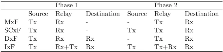
Table 2.3: Types of relaying protocols

Phase 1 Phase 2

Source Relay Destination Source Relay Destination

MxF Tx Rx - - Tx Rx

SCxF Tx Rx - Tx Tx Rx

DxF Tx Rx Rx - Tx Rx

IxF Tx Rx+Tx Rx Tx Tx+Rx Rx

During the past a few years, diﬀerent relaying strategies have been proposed and studied in order to improve the performance [2]. Some well-investigated protocols are concluded as below, where ‘x’ stands for ‘amplify’, ‘compress’, ‘decode’,etc.

• Multi-hop x Forward (MxF): In the ﬁrst hop, the source transmits, and only the relay listens. In the second hop, only the relay transmits, and the destination listens. If there are N relays, the number of hops are N + 1 between the source and destination. Dual-hop relaying is a special case of MxF.

(40)

• Diversity x Forward (DxF): In the ﬁrst phase, the source transmits, and both relay and destination are listening. In the second phase, only the relay transmits and the destination listens. Note that the destination can receive two ‘copies’ of the original information block. This protocol utilise the broadcast nature of wireless transmission.

• Intersymbol Interference x Forward (IxF): If the relay node works in full-duplex mode, IxF is applicable. In the ﬁrst hop, the source transmits one informa-tion block to the relay and destinainforma-tion. In the second phase, the relay transmits this block to destination, while receiving another block from the source. As a result, the destination is continuously listening, and in each phase hears a com-bination of the current block from the source, and the previous block from the relay simultaneously.

(41)

Chapter 3

Overview of Radio Resources and

Their Allocation Schemes

This chapter presents a literature review on RA for broadband wireless communication systems. The radio resources are introduced in Section 3.1. The existing RA schemes are described in Section 3.2 for multi-carrier based communication systems.

3.1 Radio Resources in Wireless Communications

For any of the wireless communication systems mentioned in the Chapter 2, EM wave is the solely material to carry signals. Therefore, radio resources are usually referred to the following prime elements: bandwidth, carrier frequency, and transmit power.

3.1.1 Bandwidth and Carrier Frequency

(42)

avoid the interference with other sources and keep low power density, direct sequence and frequency hopping were considered in the application. In [77], a method was devel-oped for examining the wireless services coexistence between wireless local area network (WLAN) and WPAN, where the closed-form solution for the probability of collision was derived. A spectrum sharing problem was studied in [78] for the coexistence of multiple systems, where the self-forcing protocol must correspond to an equilibrium of a game. It was proved that the repeated game is more appropriate than the one shot game to model the interaction. In [79], a uniﬁed framework was presented for interference characterisations in the unlicensed frequency bands, where a new spatial-spectral inter-ference model was introduced. In this model, interinter-ferences can be any power spectral density and are distributed according to Poisson process in space and frequency do-mains. In Chapter 5, the unlicensed 60 GHz wireless communication in a short-range scenario is considered.

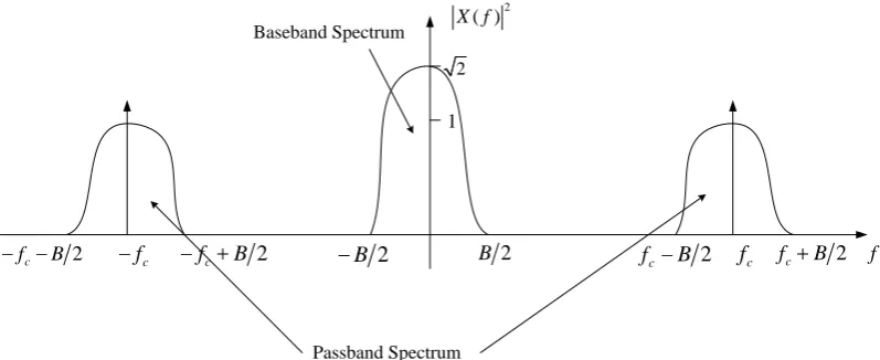
At the transmission end, the length of the antenna should be comparable with the wavelength in order to deliver the EM wave eﬃciently,i.e., a quarter of the wavelength [80]. While in the early wireless communication system, human voice is the only infor-mation source needed to be transmitted. The spectrum of human voice in telephony system is usually limited between 300 and 3,000 Hz [81], so the minimum size of the antenna should be around 25 km, which is incredibly long. To solve this problem, the baseband signal needs to be up-converted to a radio frequency (RF) waveform [24], which allows the contained information to be transmitted out by small-sized antennas. Fig. 3.1 shows the relationship between the passband and its baseband of a complex modulated signal in the frequency domain, whereB is the bandwidth,fc is the central carrier frequency. Deﬁning Xb(f) as the frequency response of the baseband signal

xb(t), the passband signalx(t) [24] can be written as

x(t) =√2R [

xb(t)ej2πfct

]

(3.1)

where R[·] is the real part of a complex number, and ej2πfct _{is the carrier waveform.}

Applying Fourier transform F{·}, the frequency response of x(t) can be deﬁned as

X(f) =F{x(t)}= √1

2{Xb(f−fc) +X

∗

b(−f −fc)} (3.2) Since the frequency response of the carrier ej2πfct _{is an impulse function,} _X₍_f_{) keeps}

(43)

f

c f c

f fc B 2 B 2 B 2 fc B 2 fc B 2

2 c

f B

2

1

2

( )

X f

[image:43.595.135.534.86.249.2]

Passband Spectrum Baseband Spectrum

Figure 3.1: Illustration of the relationship between a passband spectrum and its base-band equivalent

the carrier central frequency affects the PL, and further affects the received SNR. The higher fc is, the lower the received SNR will be. From (2.39) it is easy to observe that once the fc is fixed, the data rate for transmission is mainly determined by the bandwidth. In other words, ultra high frequency transmission can provide ultra wide band, but it also brings serious attenuation on the strength of signals.

3.1.2 Transmit Power

In order to combat with the attenuation from PL and contamination from the noise, signals need to maintain a certain level of average power at the receiving end. Therefore, the transmit power should be large enough. From (2.39), it is clear that the channel capacity is in proportion to the transmit power. Ideally, the power is expected as large as possible. However, this assumption is not realistic in the practical scenario, since there are some limitations upon the transmit power.

At the transmitter, the output power of PA that is connected to the transmit antenna provides the power of RF passband signals. Usually, this output power equals to the average power of the passband waveform. Fig. 3.2 illustrates the ampliﬁcation model of the PA with a ﬁxed gain, wherePinis the input drive power,Poutis the output power, andP1dB is the 1 dB compression point. It can be seen that there is a limit on

the linear ampliﬁcation of the PA. IfPinis greater than certain thresholds, PA will work in the nonlinear or saturation regions. IfPin is even greater than the output value of