This is a repository copy of
Model estimation of cerebral hemodynamics between blood
flow and volume changes: a data-based modelling approach
.
White Rose Research Online URL for this paper:
http://eprints.whiterose.ac.uk/74639/
Monograph:
Wei, H.L., Zheng, Y., Pan, Y. et al. (4 more authors) (2008) Model estimation of cerebral
hemodynamics between blood flow and volume changes: a data-based modelling
approach. Research Report. ACSE Research Report no. 983 . Automatic Control and
Systems Engineering, University of Sheffield
[email protected] https://eprints.whiterose.ac.uk/ Reuse
Unless indicated otherwise, fulltext items are protected by copyright with all rights reserved. The copyright exception in section 29 of the Copyright, Designs and Patents Act 1988 allows the making of a single copy solely for the purpose of non-commercial research or private study within the limits of fair dealing. The publisher or other rights-holder may allow further reproduction and re-use of this version - refer to the White Rose Research Online record for this item. Where records identify the publisher as the copyright holder, users can verify any specific terms of use on the publisher’s website.
Takedown
If you consider content in White Rose Research Online to be in breach of UK law, please notify us by
Model Estimation of Cerebral Hemodynamics Between Blood
Flow and Volume Changes: A Data-Based
Modelling Approach
H. L. Wei(a), Y. Zheng(b), Y. Pan , D. Coca(b) (a), L. M. Li(a) , J. E. W. Mayhew(b), and S. A. Billings(a)
(a) Department of Automatic Control and Systems Engineering, University of Sheffield, Mappin Street, Sheffield, S1 3JD, UK
(b) Department of Psychology, University of Sheffield, Western Bank, Sheffield, S10 2TP, UK
Research Report No. 983
Department of Automatic Control and Systems Engineering
The University of Sheffield
Mappin Street, Sheffield,
S1 3JD, UK
Model Estimation of Cerebral Hemodynamics Between Blood
Flow and Volume Changes: A Data-Based
Modelling Approach
H. L. Wei(a), Y. Zheng(b), Y. Pan , D. Coca(b) (a), L. M. Li(a) , J. E. W. Mayhew(b), and S. A. Billings(a)
(a) Department of Automatic Control and Systems Engineering, University of Sheffield, Mappin Street, Sheffield, S1 3JD, UK
(b) Department of Psychology, University of Sheffield, Western Bank, Sheffield, S10 2TP, UK
Abstract: It is well known that there is a dynamic relationship between cerebral blood flow (CBF) and cerebral blood volume (CBV). With increasing applications of functional magnetic resonance imaging (fMRI), where the blood oxygen level dependent (BOLD) signals are recorded, the understanding and accurate modelling of the hemodynamic relationship between CBF and CBV becomes increasingly important. This study presents an empirical and data-based modelling framework for model identification from CBF and CBV experimental data. It is shown that the relationship between the changes in CBF and CBV can be described using a parsimonious autoregressive with exogenous input model (ARX) structure. It is observed that neither the ordinary least squares (LS) method nor the classical total least squares (TLS) method can produce accurate estimates from the original noisy CBF and CBV data, in that the resultant ARX models may be unstable and thus cannot generate stable model predicted outputs. A regularized total least squares (RTLS) method is employed and extended to solve such an error-in-the-variables problem. Quantitative results show that the RTLS method works very well on the noisy CBF and CBV data. Finally, a combination of RTLS with a filtering method can lead to a parsimonious but very effective model that can characterize the relationship between the changes in CBF and CBV.
1. Introduction
It is well known that there is a dynamic relationship between cerebral blood flow (CBF) and cerebral blood volume (CBV) (Grubb et al., 1974; Buxton et al., 1998; Mandeville et al., 1999; Jones et al., 2001, 2002; Kong et al., 2004; Zheng et al., 2005). With the increasing applications of position emission tomography (PET) and functional magnetic resonance imaging (fMRI), where the understanding of the blood oxygen level dependent (BOLD) signal plays a key role, it is becoming increasing important to establish an accurate quantitative description of the dynamics relating CBF and CBV. The quantitative description of the relationship between changes in blood flow (volume flux per unit time through a tissue volume element) and blood volume was first presented by Grubb et al. (1974), where it was suggested that the relationship between the two variants can be described using a
function obeying a simple power-law, that is,
CBV
∝
CBF
α , withα
a constant. This has been extensively applied when modelling hemodynamic response to activation. However, due to the fact that this power-law relationship has been derived merely based on steady-state measurements, the generalization and application to activation scenarios involving transient changes may not be valid. Buxton et al. (1998) developed a biomechanical differential equation model, called the Balloon model, to describe how evoked changes in blood flow were transformed into a BOLD signal. Mandeville et al. (1999) studied the relationship between the blood flow and volume changes and presented a model in terms of resistance and capacitance in the context of the standard windkessel theory. Friston et al. (2000, 2002) proposed a unified alternative representation on the basis of Volterra kernel theory, by combining system identification and model-based approaches, to describe nonlinear responses in fMRI including the modelling of the hemodynamic relationship between CBF and CBV.Due to the complexity of the inherent neural hemodynamics for which no or very limited a priori information about the biophysical mechanisms (the model structure and the associated model parameters) is available, analytical or theoretical modelling approaches alone may not be adequate to obtain sufficiently reliable mathematical models to describe cerebral hemodynamics between CBF and CBV. As an alternative, empirical and data-based modelling approaches, which make use of both biophysical observations and identification and information techniques, provides a complementary but very powerful tool for modelling such complex systems. Regression models, including the general linear model (GLM), autoregressive with exogenous model (ARX), nonlinear regression and nonlinear network models, are among the most popular classes of representations for characterising and understanding the dynamics of fMRI responses and related signals, see for example Friston et al. (1995), Worsley and Friston (1995), Worsley et al. (1997), Panerai et al. (2000), Woolrich et al. (2001), Mitsis et al. (2004), Riera et al. (2004) and Baraldi et al. (2007), and the references therein.
linear-in-the-parameters models is that they are easy to operate, because compared with nonlinear-in-the-linear-in-the-parameters models, such models are easier to interpret physically, simpler to analyze mathematically and quicker to compute numerically using least squares based algorithms (Billings et al., 2007). In the classical least squares (LS) approach, which is the most commonly used method for solving linear regression problems, the measurements of the design matrix formed by the ‘input’ variables (independent variables) are assumed to be ‘clean’ or ‘noise-free’ (no errors); or, the errors on the measurements of the independent variables are much smaller compared with those imposed on the ‘output’ variables (dependent variables) and can therefore be ignored. In many cases, however, these assumptions may be unrealistic. When the classical least squares approach is applied to solve linear regression problems, where these assumptions are violated, the resultant least squares estimates for the associated model parameters are inevitably biased. To overcome this drawback of the ordinary least squares algorithm, Golub and Van Loan (1973, 1980) developed an efficient numerical tool, called total least squares (TLS), for solving linear regression problems, where the effects of errors on both the dependent variables and the independent variables (and thus the design matrix) are taken into account. However, unlike the ordinary least squares algorithm where the solution can be written in a compact form, the application of the total least squares algorithm involves nonlinear optimization for parameter estimation.
2. The Data-Based Modelling Framework
2.1 The NARX model
It has been proved that under some mild conditions a discrete-time or discretized continuous-time dynamical system can be described by the following difference equation model (Leontaritis and Billings 1985a, 1985b)
) ( )) ( , ), 1 ( ), ( , ), 1 ( ( )
(n f y n y n p u n u n q e n
y = − L − − L − + (1)
where , ) and are the system input, output and noise variables; p and q are the maximum
lags in the input and output, respectively; and f is some unknown linear or nonlinear mapping. It is
generally assumed that is an independent identical distributed noise sequence. A commonly
employed form of model (1) is the well-known nonlinear autoregressive with exogenous inputs (NARX) model, which was introduced by Billings and colleagues (Billings and Leontaritis, 1981; Leontaritis and Billings, 1985a, 1985b; Chen and Billings, 1989a), and which can describe a wide range of nonlinear dynamic systems and includes several other linear and nonlinear model types, including the classical Volterra, Hammerstein, Wiener, AR, and ARX models as special cases (Pearson, 1995).
) (n
u y(n e(n)
) (n e
A generic form of the NARX model, with a nonlinear degree order , is given below l
∑
= + = d i i ix n c cn y
1
0 ( )
)
( +
∑∑
+L= = d i d j i i j
i x n x n c 1 1 , ( ) ( )
∑
∑
∑
= = = + d i d i i i i i i i d i n x n x n x c 1 1 , , , 1 1 2 1 2 1 2 ) ( ) ( ) ( l l l LL L +e(n) (2)
where d= p+q and
⎩ ⎨ ⎧ + ≤ ≤ + − − ≤ ≤ − = q p k p p k n u p k k n y n xk 1 )), ( ( 1 ), ( )
( (3)
Practical applications have shown that NARX models, with a nonlinear degree order , can often
provide satisfactory approximations for most dynamical systems. The widely used autoregressive with exogenous input (ARX) model (Astrom, 1970; Ljung, 1987; Söderström and Stoica, 1989), as a
special case of the NARX model (2) where =1 and
3
≤ l
0
0=
c , is explicitly given by
l
∑
∑
= = − + − = q j j p iiy n i b u n j a n y 1 1 ) ( ) ( )
( +e(n) (4)
maximum lags p and q, the initial full model (2) may involve a great number of candidate model terms. However, experience shows that in most cases only a small number of significant model terms are necessary and thus should not be included in the final model to represent the underlying dynamics. Most candidate model terms are either redundant or make very little contribution to the system output and can therefore be removed from the model. Several efficient model structure determination and model validity test methods have been developed over the last two decades ((Billings and Voon, 1983, 1986, 1987; Leontaritis and Billings, 1987a, 1987b; Chen et al., 1989b; Billings and Fung, 1995; Billings and Zhu, 1994, 1995; Aguirre and Billings, 1995; Wei et al., 2004; Billings and Wei, 2008; Wei and Billings, 2008a; Wei et al., 2008).
Assume that a total of m significant model terms, denoted by {φ1(n),φ2(n),L,φm(n)}, have been selected from the library consisting of all the M candidate model terms. The selected m model terms can be used to form a parsimonious model
) ( )
( ) ( )
(n 1 1 n 2 2 n n
y =θφ +θφ +L+θmφm +e(n) (5)
where )φk(n are a combination of the lagged versions of the input and output variables
and (the constant may also be included). For example, for a NARX model with a nonlinear
degree order ,
) (n
u y(n)
) (n k
φ are then selected from the library L={1}U{xi(n):1≤i≤d} 3
= l
} , 1 : ) ( ) (
{xi n xj n ≤i j≤d
U U{xi(n)xj(n)xk(n):1≤i,j,k≤d},where are defined by (3). Classical
linear least squares type of algorithms may be applied to estimate the associated model parameters. )
(n xk
2.2 Regularized Total Least Squares
It is known that the classical least squares algorithms and the standard statistical analysis for these
algorithms require certain assumptions: the ‘input’ (independent) variables say φk(n)in (5) are measured without errors; or the errors imposed on the ‘input’ variables are much smaller than those imposed on the ‘output’ variables (dependent variables) say y(n) in (5) and can therefore be ignored. For many cases, this assumption may not be satisfied, and the ordinary least squares method will not work well. To solve this kind of errors-in-variables (EIV) problem, Golub and Van Loan (1973, 1980) developed the total least squares method (TLS). Over the last three decades, TLS methods have been successfully applied to solve a variety of EIV problems (Van Huffel and Vandewalle, 1991; Van Huffel, 1997; Van Huffel and Lemmerling, 2002; Markovsky and Van Huffel, 2007), including the applications to biomedical data modelling (Chen, 2000; Shou et al., 2008). In some cases, the TLS method alone, however, may not be effectively immune to the amplification effects of the noise for an ill-conditioned problem. To solve this problem, the regularized total least squares (RTLS) method was proposed by combining the well-known Tikhonov regularization (Tikhonov and Arsenin, 1977) and TLS methods, see for example Mesarovic et al. (1995), Golub et al. (1999) and Siam et al. (2004).
RTLS estimate is stated as ⎭ ⎬ ⎫ ⎩ ⎨ ⎧ + + − = 2 2 2 || || || || 1 || || min
ˆ y λ
μ (6)
wherey=[y(1),L,y(N)]T , =[θ1,L,θm]T , Φ=[ 1,L, m] with for k=1, 2,…, m, N is the number of available observations, and
T m k
k =[φ (1),L,φ (N)]
μandλ are two adjustable parameters.
Clearly, whilst the ordinary least squares minimizes a sum of squared residuals, total least-squares minimizes a sum of weighted squared residuals with a penalized term formed by the square of the parameters. If μ=0, (6) reduces to the case of the Tikhonov regularization; if μ=1 andλ=0, (6)
reduces to TLS. In the present study the adjustable parameterμ will be set to be unity, that is μ=1,
and the regulation parameterλ will be chosen by trial-and-error (see the example below for more details).
m
θ θ θ1, 2,L,
Note that the solution to RTLS (6), with respect to the unknown parameters , involves
nonlinear optimization. In the literature many nonlinear optimization approaches are available to solve such a nonlinear optimization problem. In this study, however, a simplex direct search optimization algorithm, proposed by Nelder and Mead (1965), is applied to solve the nonlinear optimization problem here. The Nelder-Mead method, first introduced by Nelder and Mead in 1965 and recently enhanced theoretically by Lagarias et al. (1998), is a powerful direct ‘derivative-free’ search algorithm, where neither the computation nor the approximation of derivatives or gradients are needed. The Mead method has enjoyed enduring popularity. Of all the direct search methods, the Nelder-Mead simplex algorithm is the one most often found in numerical software package (Lewis et al., 2000).
2.3 Choosing the Regularization Parameter
λ
The determination of the regularization parameter in RTLS (6) is a significant but difficult issue, and there is no universal criterion on how to select the parameter for general dynamical modelling problems. Some empirical or ad hoc methods, however, may work quite well when choosing such regulation parameters (Wei and Billings, 2008b). This study suggests using a trial-and-error approach
and the basic idea is as follows. Let be the LS estimate for the model parameter vector and
be the normalized mean-square-errors (NMSE) calculated from the model with the LS estimate.
A rule of thumb from our experience is to initially choose a number
(LS) ˆ ) LS ( nmse ˆ σ 2 2 ) LS ( 2 ) LS ( || || || ˆ || || ˆ || 1 1 y y e − + = 2 2 ) LS ( 2 ) LS ( || || || ˆ || || ˆ || 1 1 y y y y − − + = 2 ) LS ( ) LS ( nmse 0 || ˆ || 1 ˆ + = σ
where yis the mean of the output vector y, and are the model prediction (one-step-ahead
prediction) and the model residual vector, produced by the model with LS estimate . Using the
number (LS) ˆ e (LS) ˆ y (LS) ˆ 0
λ , define a set: Γ for k=0,1,2,3,4,5. The
regulation parameter
} 10 :
{ k 0 k = −k U{βkλ0:βk =0.5×10−k}
= α λ α
λwill be chosen from the set Γ, where each element is set to be the candidate as
the regulation parameter and the RTLS procedure is then performed. This will lead to a set of models with different RTLS estimates. The criterion for selecting the regularization parameter is to inspect the predictive capability of the resultant models. For a dynamical modelling problem, the resultant model should possess a satisfactory predicative ability in terms of model predicted output (MPO), which is an extreme case of long-term prediction and which is the most stringent test for dynamical models. The value in Γthat produces the model with the best performance (in the sense that minimizes the errors between the model predicted output and the corresponding measurements) will be selected as the regulation parameterλ.
As an example, consider two nonlinear systems described by the models below
∑
∑
= = − + − = 3 1 4 1 )] 1 ( [ ) ( ) ( j j j iiy n i b u n a
n
y (8)
∑
∑
= = − + − = 3 1 2 4 1 )] ( [ ) ( ) ( j j iiy n i b u n j a
n
y (9)
where the model parameter vector =[1.8, -2.0, 1.5, -0.5, 0.5, -0.25, -0.1] for
both of the two models above, and the input u(n) was chosen to be a stochastic process ] , , , , , ,
[a1 a2 a3 a4 b1 b2 b3 T = ) 2 ( 98 . 0 ) 1 ( 96 . 1 ) ( )
(n =w n − wn− + w n−
u (10)
where w(n) was a Gaussian white noise sequence with zero mean and unit variance. The models were simulated and two hundred input-output data pairs were collected for both of the two models; a noise signal was then deliberately added to the data points, and these noisy data were then used for model parameter estimation using the RTLS algorithm.
Table 1. A comparison of the parameter estimates produced by LS, TLS and RTLS, for the model given by (8).
a a a a b b b Noise level and the
regularization parameter in RTLS
1 2 3 4 1 2 3
True 1.8 -2.0 1.5 -0.5 0.5 -0.25 -0.1
LS 1.7958 -1.9938 1.4934 -0.4947 0.4942 -0.2489 -0.0982 SNR=40dB (for input)
TLS 1.7988 -1.9981 1.4978 -0.4984 0.5015 -0.2498 -0.1034 SNR=40dB (for output)
λ=3.3704 8
10−
×
RTLS 1.8005 -2.0011 1.5005 -0.4991 0.4956 -0.2484 -0.0984
LS 1.5291 -1.5649 1.1044 -0.2943 0.4583 -0.2817 -0.1095 SNR=20dB (for input)
TLS 1.7736 -1.9637 1.4529 -0.4650 0.4894 -0.2471 -0.0566 SNR=20dB (for output)
λ=4.0654 6
10−
×
RTLS 1.7919 -2.0191 1.5311 -0.5125 0.5365 -0.2553 -0.1225
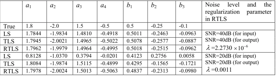
Table 2. A comparison of the parameter estimates produced by LS, TLS and RTLS, for the model given by (9).
a a a a b b b Noise level and the
regularization parameter in RTLS
1 2 3 4 1 2 3
True 1.8 -2.0 1.5 -0.5 0.5 -0.25 -0.1
LS 1.7844 -1.9834 1.4810 -0.4918 0.5011 -0.2463 -0.0963 SNR=40dB (for input)
TLS 1.7945 -2.0021 1.4965 -0.5022 0.5078 -0.2577 -0.0887 SNR=40dB (for output)
λ=2.2730 6
10−
×
RTLS 1.7962 -1.9979 1.4964 -0.4995 0.5018 -0.2515 -0.0962
LS 0.8128 -1.0370 0.3794 -0.0201 0.4123 0.2756 0.0058 SNR=20dB (for input)
TLS 1.8084 -1.9874 1.5115 -0.4899 0.4295 -0.1565 -0.1721 SNR=20dB (for output)
λ=0.0011 RTLS 1.7978 -2.0024 1.5013 -0.5063 0.4837 -0.2313 -0.0980
3. Data Modelling Between CBF and CBV
3.1 The Datasets
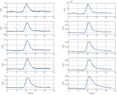
In this work, changes in CBF were measured using laser-Doppler flowmetry (LDF), with a sampling rate of 30Hz, while changes in CBV were measured using optical imaging spectroscopy (OIS), with a sampling rate of 7.5Hz. For convenience of data modelling, the CBF data were then downsampled at 7.5Hz. Brief 2s stimuli of 1, 2, 3, 4, and 5Hz were randomly interleaved and applied within a single experimental run with stimulus intensity of 1.2mA and a pulse width of 0.3ms. Thirty trials were obtained for each stimulus condition with each trial lasting 23s (with stimulus onset at 8s), and an inter-trial-interval of 25s to avoid hemodynamic refractory period. A more detailed description of the experiments and the associated data sets can be found in Martindale et al (2003) and Kong et al. (2004).
[image:10.595.77.520.291.413.2]Fig. 1. Measurements of changes in CBF and CBV. From top to bottom, the plots are for the cases of 1, 2, 3, 4, and 5Hz.
3.2 Model Identification
A model term and variable selection algorithm (Wei et al., 2004) was performed over each of the five datasets, and the significant model variables were determined to be x1(t)=y(t-1), x2(t)=y(t-2), x3(t)=u(t), x4(t)=u(t-1), and x5(t)=u(t-2). Three types of NARX models were considered: i) An ARX
model given by (4); ii) A NARX model with a nonlinear degree order =2; and iii) A NARX model
with a nonlinear degree order =3. The initial full models of all the three types were formed using the five selected significant model variables. Each of the three initial full models was then used to generate a parsimonious model that fits all the five data sets, and this was implemented by using a common model structure selection algorithm (Wei et al., 2008) over the five datasets. By comparing the resultant model performance and by following the parsimonious principle, the common model structure that fits all the five datasets was determined to be
l
l
) 2 ( ) 1 ( ) ( ) 2 ( ) 1 ( )
(n =a1y n− +a2y n− +b0u n +b1u n− +b2u n−
y (11)
where the estimates of the coefficients (i=1,2) and (j=0,1,2) using LS, TLS, and RTLS, for the
five cases of 1, 2, 3, 4, and 5Hz, are shown in Table 3.
i
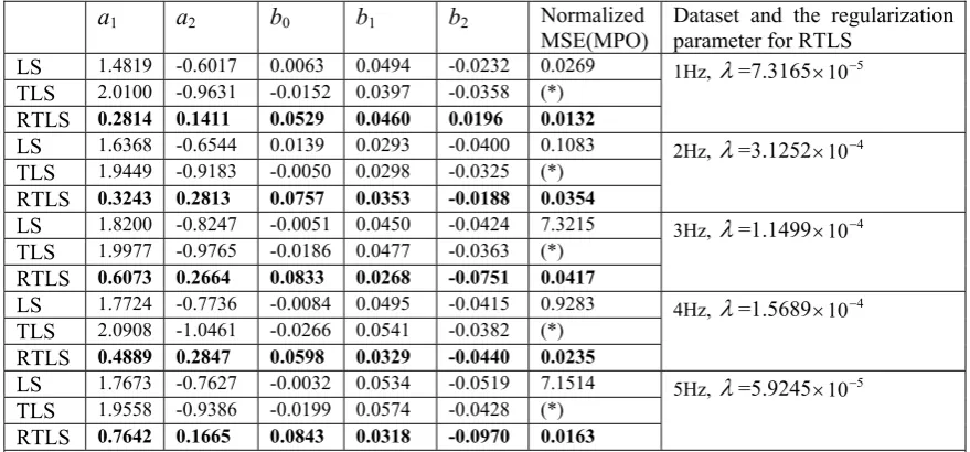
Table 3. The parameter estimates produced by LS, TLS and RTLS, for the CBF and CBV modelling problem.
a a b b b Normalized
MSE(MPO)
Dataset and the regularization parameter for RTLS
1 2 0 1 2
LS 1.4819 -0.6017 0.0063 0.0494 -0.0232 0.0269
TLS 2.0100 -0.9631 -0.0152 0.0397 -0.0358 (*)
λ=7.3165 5
10−
×
1Hz,
RTLS 0.2814 0.1411 0.0529 0.0460 0.0196 0.0132
LS 1.6368 -0.6544 0.0139 0.0293 -0.0400 0.1083
TLS 1.9449 -0.9183 -0.0050 0.0298 -0.0325 (*)
λ=3.1252 4
10−
×
2Hz,
RTLS 0.3243 0.2813 0.0757 0.0353 -0.0188 0.0354
LS 1.8200 -0.8247 -0.0051 0.0450 -0.0424 7.3215
TLS 1.9977 -0.9765 -0.0186 0.0477 -0.0363 (*)
λ=1.1499 4
10−
×
3Hz,
RTLS 0.6073 0.2664 0.0833 0.0268 -0.0751 0.0417
LS 1.7724 -0.7736 -0.0084 0.0495 -0.0415 0.9283
TLS 2.0908 -1.0461 -0.0266 0.0541 -0.0382 (*)
λ=1.5689 4
10−
×
4Hz,
RTLS 0.4889 0.2847 0.0598 0.0329 -0.0440 0.0235
LS 1.7673 -0.7627 -0.0032 0.0534 -0.0519 7.1514
TLS 1.9558 -0.9386 -0.0199 0.0574 -0.0428 (*)
λ=5.9245 5
10−
×
5Hz,
RTLS 0.7642 0.1665 0.0843 0.0318 -0.0970 0.0163
(*): the model produced by TLS is instable and the associated model predicted output (MPO) is divergent; MSE(MPO): the normalized mean-square error was calculated for the associated model predicted output (that is different from short-term predictions).
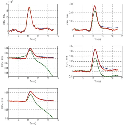
By setting the first two observations of CBV (the output) as the initial condition and by using the observations of the CBF as the inputs, the models produced by the LS and RTLS algorithms were simulated. The associated model predicted outputs (MPO) are shown in Fig. 2. Note that MPO here is different from short-term (or multi-step) ahead predictions, and is a far more severe test than the often used one-step ahead (OSA) predictions since the latter can often look good even for very poor models. From Table 3 and Fig. 2, the following conclusions can be drawn: i) For the given real datasets, where the associated measurements of changes in CBF and CBV may be contaminated by noise, the ordinary LS method does not work well; neither does the TLS method; ii) The RTLS method significantly outperforms both the LS and TLS methods, in that it can very effectively handle the errors-in-variables problems here; iii) The proposed empirical choice of the regularization parameter
λ given by (7) works very well for the RTLS algorithm.
3.3 Data Filtering
Fig. 2. Comparisons of the model predicted outputs (MPO) from the LS and RTLS related models (given in Table 3) and the associated measurements, for the five cases of 1, 2, 3, 4, and 5Hz. In each figure, the thin-solid line indicates the measurement, the thick-solid line indicates the MPO produced by the RTLS related model, and the thick-dashed line indicates the MPO produced by the LS related model.
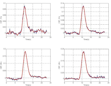
The original CBF data in all the five datasets were filtered with Daubechies’ wavelets (Daubechies, 1992). The filtered data, along with the relevant original data for the first four cases of 1, 2, 3, and 4 Hz, are shown in Fig. 3 (the 5Hz case was omitted here to save space). Using the filtered CBF data as the input and the associated CBV data (unfiltered) as the output, the coefficients of the ARX model of the form (11) were then re-estimated using the RTLS method, and the associated parameter estimates are shown in Table 4.
[image:13.595.91.496.111.533.2]original CBV data. Comparisons between the model predicted outputs and the corresponding original observations are shown in Fig. 4. From Table 4 and Fig. 4, it is quite clear that models estimated from the filtered CBF data are much better than those estimated from the original CBF data. While Fig. 4. only provides some visual perception, the values of the normalized MSE listed in Table 4 and Table 3 gives a quantitative comparision. As can be noticed, the normalized MSE for the model predicted output given in Table 4 is much smaller than that given in Table 3, for all the five cases.
Table 4. The RTLS estimates for CBF and CBV modeling problem, where the filtered CBF data as the input and the original CBV data (unfiltered) as the output.
a a b b b Normalized
MSE(MPO)
Dataset and the regularization parameter for RTLS
1 2 0 1 2
RTLS 0.2948 0.1929 0.0901 0.0134 0.0023 0.0133 λ=5.2565 5
10−
×
1Hz,
RTLS 1.0085 -0.0273 0.0093 0.1775 -0.1816 0.0157 2Hz, λ=1.0357×10⁻⁶ RTLS 0.9872 -0.0164 0.1024 -0.0018 -0.0910 0.0086 λ=2.2285 6
10−
×
3Hz,
RTLS 0.8348 0.1180 0.0258 0.1395 -0.1540 0.0059 λ=2.8804 6
10−
×
4Hz,
RTLS 0.6617 0.3001 0.1153 0.0308 -0.1343 0.0027 λ=5.9841 6
10−
×
5Hz,
Model predicted output (MPO) was calculated by simulating the associated model where the original CBF data (unfiltered) was set to be the input, and the model predicted output was then compared with the original real measurement.
[image:14.595.103.493.394.698.2]Fig. 4. Comparisons between the measurements and the associated model predicted outputs produced by the models estimated from the filtered CBF data using the proposed RTLS algorithm. The thin-solid lines indicate the measurements, and the thick-dashed lines indicate the associated model predicted outputs.
3.4 Continuous-Time Models
In some cases it may be desirable to identify continuous-time models. From linear systems and signal processing theory, the linear discrete-time model (11) can easily be converted into a continuous model. First, the discrete-time (z-domain) transfer function of (11) is given by
2 2 1 1
2 2 1 1 0
1 )
( − −
− −
− −
+ + =
z a z a
z b z b b z
H (12)
By applying the well-known Tustin transform (also called the bilinear transform), that is, by letting
2 / 1
2 / 1
s s sT
sT sT e
z s
− + ≈
= (13)
-domain. Taking the case of 5Hz as an example, where =2/15s, and the associated coefficients are
listed by Table 4, the s-domain transfer function is given by
s T
316 . 6 65 . 28
965 . 1 501 . 5 03654 . 0 )
( 2
2
5 + +
+ +
− =
s s
s s
s
G (14)
The transfer function (14) can further be converted into a differential equation model below
) ( 965 . 1 501 . 5 03654
. 0 ) ( 316 . 6 65 .
28 2
2
2 2
t u dt
du dt
u d t
y dt
dy dt
y
d + + =− + +
(15)
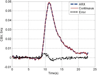
[image:16.595.105.486.385.679.2]Driven by the input (measurement of changes in CBF) in the associated dataset of the 5Hz case, the continuous-time model (14) was simulated by using an extrapolation method in the Runge-Kutta family of ordinary differential equation (ODE) solvers provide by Matlab in the ordinary differential equation toolbox, and a comparison of the output produced by the continuous-time model (14) and that produced by the discrete-time model given in Table 4 is shown in Fig. 5.
4. Discussion and Conclusions
The focus of the work has been on the development of a data-based modelling approach for the identification of models that can be used to describe the dynamical relationship of changes in CBF and CBV during neural activity. This is a complicated black-box system where the true model structure is unknown and thus needs to be identified from available experimental data. The central task of data-based modelling of such a structure-unknown system involves several aspects including model variable selection, model structure specification and detection, parameter estimation, and model validation. In this study, a nonlinear autoregressive with exogenous input model (NARX), which has been widely used for nonlinear system identification, was chosen as the initial candidate model structure. Compared with many other model structures for example typical neural networks, the NARX model structure possesses several advantages, some of which are:
A wide range of nonlinear systems can be described using the NARX model.
•
Over the last two decades the NARX model has been systematically studied and a series of excellent algorithms have been developed for the identification such models. This means that model structure detection and parameter estimation for such a model can be performed speedily and efficiently using existing algorithms.
•
The NARX model is transparent and thus can easily be related back to the underlying system.
•
Algorithms that exist can directly map the NARX model and continuous-time nonlinear differential equation (ODE) models into the frequency domain (Peyton-Jones and Billings, 1989, 1990; Lang and Billings, 1996); this allows the user to reveal the explicit link from the time-domain model parameters to the frequency-domain properties.
•
For the model parameter estimation problem it has been illustrated that neither the ordinary least squares (LS) method nor the classical total least squares (TLS) method can produce reliable estimates from the available CBF and CBV data, which were contaminated by noise. The regularized total least squares (RTLS) method, however, works very well when applied to the error-in-variables problem here. Note that the application of RTLS involves nonlinear optimization and the need to estimate the value of the regularization parameter. The Nelder-Mead simplex direct search optimization algorithm was introduced to solve the RTLS equation (6), where the initial value of the unknown parameters was chosen to be the LS estimates. While the Nelder-Mead algorithm, coupled with the rule of thumb (Eq. (7)) for choosing the regularization parameter, can work very well for model parameter estimation, there still exists a space to further optimize the choice of the regularization parameter, as well as the initial value for the free parameters to be optimized.
Acknowledgements
The authors gratefully acknowledge that this work was supported by the Engineering and Physical Sciences Research Council (EPSRC), U.K.
References
L. A. Aguirre, S. A. Billings. Dynamical effects of overparametrization in nonlinear models. Physica D, 80, pp.26-40, 1995.
K. J. Astrom. Introduction to Stochastic Control Theory. Academic Press, New York, 1970.
P. Baraldi, A. A. Manginelli, M. Maieron, D. Liberati, C. A. Porroa. An ARX model-based approach to trial by trial identification of fMRI-BOLD responses. Neuroimage, 37, pp.189–201, 2007. S. A. Billings, C. F. Fung. Recurrent radial basis function networks for adaptive noise cancellation.
Neural Networks, 8, pp.273–290, 1995.
S. A. Billings, I. J. Leontaritis. Identification of nonlinear systems using parametric estimation techniques. Proc. IEE Conf. Control and its Applications, Warwick, pp. 183–187, 1981.
S. A. Billings, W. S. F. Voon. Structure detection and model validity tests in the identification of non-linear system. Proc. Institution of Electronic Engineers, Pt D, 130, pp.193–199, 1983.
S. A. Billings, W. S. F. Voon. Correlation based model validity tests for non-linear models. Int. J. Control, 44, pp.235–244, 1986.
S. A. Billings, W. S. F. Voon. Piecewise linear identification of non-linear systems. Int. J. Control, 46, pp.215–235, 1987.
S. A. Billings, H. L. Wei, M. A. Balikhin. Generalized multiscale radial basis function networks.
Neural Networks, 20, pp.1081-1094, 2007.
S. A. Billings, H. L. Wei. An adaptive orthogonal search algorithm for model subset selection and
non-linear system identification. Int. J. Control, 81, pp. 714–724, 2008.
S. A. Billings, Q. M. Zhu. Nonlinear model validation using correlation tests. Int. J. Control, 60, pp.1107–1120, 1994.
S. A. Billings, Q. M. Zhu. Model validation tests for multivariable nonlinear models including neural networks. Int. J. Control, 62, 749–766, 1995.
R. B. Buxton, E. C. Wong, L. R. Frank. Dynamics of blood flow and oxygenation changes during brain activation: the balloon model. Magn Reson Med, 39, pp.855–864, 1998.
S. W. Chen. A two-stage description of cardiac arrhythmias using a total least squares-based prony modeling algorithm. IEEE Trans. Biomedical Engineering, 47, pp.1317-1327, 2000.
S. Chen, S. A. Billings. Representation of non-linear systems: the NARMAX model, Int. J. Control, 49, pp.1013-1032, 1989a.
S. Chen, S. A. Billings, W. Luo. Orthogonal least squares methods and their application to nonlinear system identification. Int. J. Control, 50, pp. 1873–1896, 1989b.
K. J. Friston. Bayesian estimation of dynamical systems: an application to fMRI. NeuroImage, 16, pp.513– 530, 2002.
K. J. Friston, A. Mechelli, R. Turner, C. J. Price. Nonlinear responses in fMRI: the balloon model, volterra kernels and other hemodynamics. Neuroimage, 12, pp.466–477, 2000.
K. J. Friston, A. P. Holmes, J. B. Poline, P. J. Grasby, S. C. Williams, R. S. Frackowiak, R. Turner. Analysis of fMRI time-series revisited. NeuroImage, 2, pp.45–53, 1995.
G. H. Golub. Some modified matrix eigenvalue problems. SIAM Rev. 15, 318–344, 1973.
G. H. Golub, P. C. Hansen, D. P. O’Leary. Tikhonov regularization and total least squares. SIAM J. Matrix Analysis and Applications, 21, pp.185–194, 1999.
G. H. Golub, C. F. Van Loan. An analysis of the total least squares problem. SIAM J. Numer. Anal. 17, 883–893, 1980.
R. L. Grubb, M. E. Raichle, J. O. Eichling, M. M. Ter-Pergossian. The effects of changes in PACO2 on cerebral blood volume, blood flow and vascular mean transit time. Stroke, 5, pp.630–639, 1974. M. Jones, J. Berwick, D. Johnston, J. Mayhew. Concurrent optical imaging spectroscopy and
laser-Doppler flowmetry: the relationship between blood flow, oxygenation, and volume in rodent barrel cortex. Neuroimage, 13, pp.1002–1015, 2001.
M. Jones, J. Berwick, J. Mayhew. Changes in blood flow, oxygenation, and volume following extended stimulation of rodent barrel cortex. Neuroimage, 15, pp.474–487, 2002.
Y. Kong, Y. Zheng, D. Johnston, J. Martindale, M. Jones, S. Billings, J. Mayhew. A model of the dynamic relationship between blood flow and volume changes during brain activation. J. Cereb. BloodFlow Metab., 24, pp.1382–1392, 2004.
Z. Q. Lang, S. A. Billings. Output frequency characteristics of nonlinear systems. Int. J. Control, 64, pp.1049–1067, 1996.
J. Lagarias, J. A. Reeds, M. H. Wright, P. E. Wright. Convergence properties of the Nelder–Mead simplex method in low dimensions. SIAM J. Optim., 9, pp. 112–147, 1998.
I. J. Leontaritis, S. A. Billings. Input–output parametric models for non-linear systems—part I: Deterministic non-linear systems. Int. J. Control, 41, pp.303–328, 1985a.
I. J. Leontaritis, S. A. Billings. Input–output parametric models for non-linear systems—part II: Stochastic non-linear systems. Int. J. Control, 41, pp.329–344, 1985b.
I. J. Leontaritis and S. A. Billings. Model selection and validation methods for non-linear systems.
Int. J. Control, 45, pp. 311–341, 1987a.
I. J. Leontaritis and S. A. Billings. Experimental-design and identifiability for non-linear systems. Int. J. Systems Science, 18, pp. 189–202, 1987b.
R. M. Lewis, V. Torczon, M. W. Trosset. Direct search methods: then and now. J. Computational and Pllied Mathematics, 124, pp.191-207, 2000.
L. Ljung. System Identification: Theory for the User. Englewood Cliffs : Prentice-Hall, 1987.
Evidence of a cerebrovascular postarteriole Windkessel with delayed compliance. J. Cereb. Blood Flow Metab, 19, pp.679–689, 1999.
J. Martindale, J. Mayhew, J.Berwick, M. Jones, C. Martin, D. Johnston, P. Redgrave and Y. Zheng. The hemodynamic impulse response to a single neural event. J Cereb Blood Flow Metab, 23, pp.546-555, 2003.
V. Mesarovic, N. Galatsanos, A. Katsaggelos. Regularizad constrained total least squares image restoration, IEEE Trans. Image Process, 4, pp.1096–1108, 1995.
I. Markovsky, S. Van Huffel. Overview of total least squares methods. Signal Processing, 87, pp.2283-2302, 2007.
G. D. Mitsis, M. J. Poulin, P. A. Robbins, V. Z. Marmarelis. Nonlinear modeling of the dynamic effects of arterial pressure and co2 variations on cerebral blood flow in healthy humans. IEEE Trans. Biomed. Eng., 51, pp.1932–1943, 2004.
J. A. Nelder, P. Mead. A simplex method for function minimization. Computer Journal, 7, pp.308-313, 1965.
R. B. Panerai, D. M. Simpson, S. T. Deverson, P. Mahony, P. Hayes, D. H. Evans. Multivariate dynamic analysis of cerebral blood flow regulation in humans. IEEE Trans. Biomed. Eng., 47, pp.419–423, 2000.
R. K. Pearson, Discrete-Time Dynamic Models, New York: Oxford University Press, 1999.
J. C. Peyton-Jones, S. A. Billings. Recursive algorithm for computing the frequency response of a class of non-linear difference equation models. Int. J. Control, 50, pp.1925-1940, 1989.
J. C. Peyton-Jones, S. A. Billings. Interpretation of non-linear frequency response functions. Int. J. Control, 52, pp.319-346, 1990.
J. Riera, J. Bosch, O. Yamashita, R. Kawashima, N. Sadato, T. Okada, T. Ozakic. fMRI activation maps based on the NN-ARx model. Neuroimage, 23, pp.680–697, 2004.
G. F. Shou, L. Xia, M. F. Jiang, Q. Wei, F. Liu, S. Crozier. Truncated total least squares: A new regulation method for the solution of ECG inverse problems. IEEE Trans. Biomedical Engineering, 55, pp.1327-1335, 2008.
D. M. Sima, S. Van Huffel, G. H. Golub. Regularized total least Squares based on quadratic eigenvalue problem solvers. BIT Numer. Math. 44, pp.793–812, 2004.
T. Söderström, P. Stoica. System Identification. New York : Prentice Hall, 1989
A. N. Tikhonov, V. Arsenin. Solution of Ill-Posed Problems.New York: Wiley & Sons, 1977.
S. Van Huffel (Ed.). Recent advances in total least squares techniques and errors-in-variables modeling. SIAM Proceedings Series, SIAM, Philadelphia, 1997.
S. Van Huffel, P. Lemmerling (Eds.). Total Least Squares and Errors-in-variables Modeling: Analysis, Algorithms and Applications. Kluwer Academic Publishers, Dordrecht, 2002.
S. Van Huffel, I. Markovsky, R. J. Vaccaro, T. Soderstrom (Guest Eds.). Total least squares and errors-in-variables modeling. Signal Processing, 87, pp. 2281–2490, 2007.
H. L. Wei, S. A. Billings, J. Liu. Term and variable selection for non-linear system identification. Int.
J. Control, 77, pp. 86–110, 2004.
H. L. Wei, S. A. Billings. Model structure selection using an integrated forward orthogonal search algorithm assisted by squared correlation and mutual information. Int. J. Modelling, Identification and Control, 2008a (in press).
H. L. Wei, S. A. Billings.Improved model identification for non-linear systems using a random subsampling and multifold modelling (RSMM) approach. Int. J. Control, 2008b (in press).
H. L. Wei, Z. Q. Lang, S. A. Billings. Identification of nonlinear parameter-dependent common structured models to accommodate varying experimental conditions and design parameter properties. Int. J. Modelling, Identification and Control, 2008 (in press).
M. W. Woolrich, B. D. Ripley, M. Brady, S. M. Smith. Temporal autocorrelation in univariate linear modeling of fMRI data. NeuroImage, 14, pp.1370–1386, 2001.
K. J. Worsley, K. J. Friston. Analysis of fMRI time-series revisited-again. NeuroImage, 2, pp.173–181, 1995.
K. J. Worsley, J.-B. Poline, K. J. Friston, A. C. Evans. Characterizing the response of PET and fMRI data using multivariate linear models. NeuroImage, 6, pp.305–319, 1997.