Some problems in testing for modality

THESES SIS/LIBRARY TELEPHONE: +61 2 6125 4631

R.G. MENZIES LIBRARY BUILDING NO:2 FACSIMILE: +61 2 6125 4063

THE AUSTRALIAN NATIONAL UNIVERSITY EMAIL: [email protected] CANBERRA ACT 0200 AUSTRALIA

USE OF THESES

This copy is supplied for purposes

of private study and research only.

Passages from the thesis may not be

copied or closely paraphrased without the

Matthew Gerard York

A thesis submitted for the degree of Doctor of Philosophy of

The Australian National University

Unless otherwise specified in the text, this thesis described my own work, supervised by Professor P.G. Hall.

A ck n o w led g em en ts

Firstly, I would like to thank my supervisor, Peter Hall, for his generosity, kindness, guidance and encouragement. His assistance has been invaluable and greatly appre­ ciated. The financial assistance of an Australian Postgraduate Award and an ANU

Supplementary Scholarship is gratefully acknowledged.

Special thanks go to all my friends and family, especially my mother, for their constant support during the preparation of this thesis.

The topic of this thesis is testing for modality. Chapter 1 provides an introduction to

the thesis and gives a survey of the existing literature on the problem of testing for modality. One of the most widely used techniques for mode testing is Silverman’s critical bandwidth test. This bootstrap test is known to be conservative and in Chapter 2 we propose a means of calibrating the bandwidth test to improve its level

accuracy. We describe the general properties of our calibrated form of the test and develop theory describing the test. We also address the problem of testing for the number of modes of a density in a compact interval, rather than over the whole real line. In Chapter 3 we quantify the conservatism of Silverman’s test and we study the numerical performance of our proposed test in an extensive simulation study. The test is applied to real data sets in Chapter 4. Chapter 5 deals with the related problem of estimating the components in a mixture of smooth regression curves. We develop an algorithm which employs local linear methods to estimate the curves

nonparametrically. We propose bandwidth selectors based on plug-in ideas. We use our calibrated test for modality to determine the number of components in the mixture.

C o n te n ts

D e cla r a tio n

A c k n o w le d g e m e n ts

A b str a ct

1 In tr o d u c tio n

1.1 Introduction... 1.2 Bump h u n tin g ... 1.3 Silverman’s critical bandwidth test ...

1.4 The DIP t e s t ... 1.5 Excess mass estimates and t e s t s ... 1.6 The mode tree and mode existence t e s t ... 1.7 Mode testing in higher dimensions... 1.8 Finite mixture d is trib u tio n s...

2 C a lib ra tin g S ilv er m a n ’s te s t

2.1 Introduction...

2.2 The bootstrap t e s t ... 2.3 Consistency of the t e s t ... 2.4 Spurious modes and compact in te r v a ls ... 2.5 Testing for j m o d es... 2.6 Theoretical results ...

2.6.1 Separation of the modes of f h ... 2.6.2 Distribution of hCTjt under H0 ... 2.6.3 Bootstrap distribution of h*cr[t/h crjt under H0

2.6.4 Distribution of hcv-lt and h*crit/h CTjt under Hi

2.6.5 Alternative regularity conditions...36

2.7 Technical a rg u m e n ts ...36

2.7.1 Proof of Theorem 2 .1 ... 36

2.7.2 Proof of Theorem 2 .2 ... 37

2.7.3 Proof of Theorem 2 .3 ... 40

2.7.4 Proof of Theorem 2 .4 ... 43

2.7.5 Proof of Theorem 2 .5 ... 44

3 N u m e r ic a l p r o p e r tie s 48 3.1 Introduction...48

3.2 Calibration ...48

3.3 Large-sample behaviour of the test ... 55

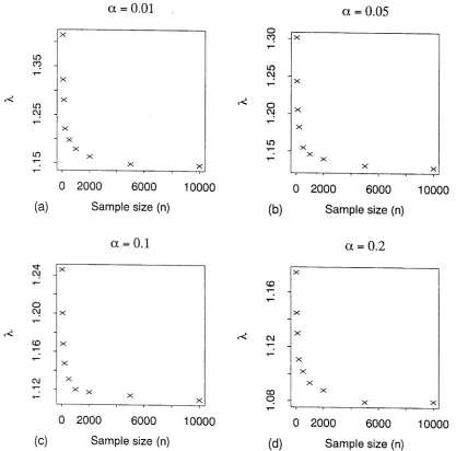
3.4 Behaviour of the test on Normally distributed samples of finite size . 60 3.4.1 Effect of sample s i z e ... 60

3.4.2 Effect of the choice of the interval X ...62

3.5 Corrections to reduce c o n serv atism ... 66

3.6 Performance of the corrections... 70

3.7 Calibrating the test for hnite sample sizes ...77

3.8 Power of the t e s t ...82

4 E x a m p le s 98 4.1 Introduction... 98

4.2 Chondrite d a t a ... 100

4.3 Buffalo snowfall d a t a ... 103

4.4 Swiss bank notes d a t a ...106

4.5 Stamp d a t a ... I l l 4.6 Galaxy velocity d a t a ... 117

5 M ix tu r e d a ta and curve e stim a tio n 122 5.1 Introduction... 122

5.2 Estimating two means in a m ix tu r e ... 122

5.3 Nonparametric curve estimation with mixture d a t a ...127

5.4 Bandwidth selection ... 132

CONTENTS VI

I n tro d u c tio n

1.1

In tro d u c tio n

This thesis is primarily concerned with assessing the modality of a population. Since most commonly considered density functions are unimodal, the presence of more than one mode is generally interpreted as a sign that the data are clustered. By

clustered, we mean that the population from which the data are drawn is not homo­ geneous but instead is made up of a number of more homogeneous subpopulations. We are interested in formally testing whether structure that appears in data sets re­ flects true features of the underlying density function. We focus our attention on the important case of testing whether a populations is homogeneous, with a unimodal density function, or whether it is multimodal.

The assessment of modality plays an important role in many applications, rang­ ing from the study of fundamental scientific theories about the structure of the

universe and the existence of new elementary particles to understanding curious features of collectables. For example, Roeder (1990) examined the distribution of

the velocities of a sample of galaxies. The velocity of a galaxy is an indication of its distance from the Earth. Astronomers predicted that gravitational attraction would lead to some clustering. Roeder’s analysis of these data indicates that the data are highly multimodal. This suggests the existence of superclusters of galaxies, surrounded by large voids. The forces causing this large-scale clustering cannot be entirely explained by existing theory. Hence in this case the detection of multi­

modality has confirmed the need for a reassessment of current theories.

Good and Gaskins (1980) investigated the existence of modes and bumps in

CHAPTER, 1. INTRODUCTION 2 mass spectra in high-energy physics scattering experiments. The detection of modes and bumps can give evidence of the existence of new elementary particles. The discovery of bimodality in lipid data by Scott et al. (1980) has led to clarification of the roles of certain risk factors in coronary artery disease (Scott, 1980). Izenman

and Sommer (1988) examined the distribution of the thickness of stamps from a nineteenth century Mexican stamp issue and deduced from the highly multimodal structure of the density function that the stamp issue had been printed on a greater

number of different types of paper than had previously been thought by collectors. Traditionally, mixture distributions have been used to model multimodal dis­ tributions. The assessment of modality is often an important part of the analysis of mixture models since it gives an indication of the number of components in the mixture. Knowing the likely number of modes of a density can also be very useful in nonparametric density estimation. Bump hunting and mode testing reveal im­ portant features in a population and we would normally want to choose the amount of smoothing of a nonparametric density estimator so that the estimate exhibits these features. Cuevas and Gonzales-Manteiga (1991) describe methods of band­

width selection for kernel density estimators that match the number of modes of the estimated and true densities.

In the remainder of this chapter we shall give a survey of existing methods for bump hunting and assessing the modality of a population. We shall mainly restrict our attention to univariate populations. In Section 1.7 we shall look at techniques for generalising these univariate approaches to higher dimensional problems. Finite mixture distributions and their connections with assessing multimodality will be described in Section 1.8.

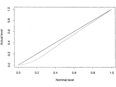
Silverman’s (1981, 1983) critical bandwidth test is the most popular nonpara­

metric technique for testing for multimodality but it is well known that the test is very conservative, in the sense that its actual level tends to be much less than its

nominal one. In Chapter 2 we propose a means of calibrating the test to improve its level accuracy and increase its power. We also address the problem of testing for the number of modes of a density in a compact interval. In the past only the

develop theory that shows that our calibration method produces a test that has asymptotically correct level.

Chapter 3 focuses on numerical aspects of the test. We quantify the conservatism of Silverman’s test and we calculate the corrections that are required calibrate the test. Through an extensive simulation study we aim to obtain a greater understand­

ing of the test and to assess the performance of our methods. We also examine the improvement in the power of the test that our calibration methods deliver.

The test is applied to a number of real data sets in Chapter 4 in order to illustrate the effectiveness of our methods for data analysis.

In Chapter 5 we consider the closely related problem of estimating the compo­ nents in a mixture of two smooth regression curves. We develop an algorithm for estimating smooth curves from mixture data and propose a technique for determin­

ing the presence of a mixture for regression data.

1.2

B u m p h u n tin g

Testing for the existence of modes can be thought of as a subproblem in a wider area of interest, that of bump hunting. In one dimension we shall define a mode of a density / to be a point where f ' ( x ) = 0 and f " ( x ) < 0. A bump will be an interval over which f " ( x ) < 0. Hence a bump does not necessarily contain a mode but a mode is always located on a bump. Cox (1966) proposed a method for testing the existence of bumps on a histogram and Good and Gaskins (1980) developed

a procedure for testing for the existence of a bump using smooth nonparametric density estimates.

Good and Gaskins’ procedure is based on estimating the density, then locally smoothing away each bump, one at a time, in order to assess the significance of each bump. Good and Gaskins (1980) used the method of maximum penalised likelihood (Good and Gaskins, 1971) to estimate the density. For an independent and identically distributed sample A b ,... , X ni the maximum penalised likelihood estimator f is the function / that maximises the penalised likelihood, defined by

n

L ( f ) = Y [ f ( X i ) e - * U \

i- 1

CHAPTER 1. INTRODUCTION 4 or equivalently, maximises the penalised log-likelihood,

n

= <-(/) = L ( f)- * ( /) = E loS / ( ^ ) - * ( /) . (1-2) z= 1

where L denotes the log-likelihood and <$(/) is a roughness penalty. The first term, L, is a measure of the goodness-of-fit to the data and the penalty measures the

smoothness of / . Without the roughness penalty the maximiser / would be a col­ lection of spikes at each of the data points. The roughness penalty imposes a degree of smoothness on the density estimate. Hence, maximising penalised likelihood is

a trade-off between smoothness and goodness-of-fit. For more details on maximum penalised likelihood as a technique for probability density estimation, see Chapter 4 of Tapia and Thompson (1978) and Section 5.4 of Silverman (1986).

Good and Gaskins (1980) use the roughness penalty

$ ( /) = ß J {7"(x)}2dx,

where 7(2;) = { /(x )} 1/2 and ß is a positive smoothing parameter that needs to be determined. Large values of ß will result in a density estimate with increased smoothness at the expense of goodness-of-fit to the data and smaller values of ß will yield bumpier estimates that provide a closer fit to the data.

The roughness penalty has a simple Bayesian interpretation which is useful for assessing the significance of a bump. We can regard jn equation (1.1) as being proportional to an improper prior density over the space of smooth functions

/ , so the smoothing parameter ß is a hyperparameter, a parameter of the prior. The penalised log-likelihood L can then be shown to correspond, up to a constant, to the logarithm of the posterior density. Thus the maximised penalised likelihood estimator / is the mode of the posterior density over the space of smooth functions

(Silverman, 1986, p. 119).

Good and Gaskins (1971, 1980) employ orthogonal series to estimate y(x). This method makes use of the expansion

r —1

7(z) =

X]

m—0

r. In theory r is infinite but in practice it needs to be terminated in the inter­ ests of computational efficiency. The series is not being terminated to control the

smoothness of / , this is entirely the work of the smoothing parameter, ß.

To implement this method it is necessary to select the value of the smoothing parameter ß. This could be done using cross-validation but Good and Gaskins opt for a technique based on goodness-of-fit statistics, in particular the x2 and the Kolmogorov-Smirnov statistics. Let S be a goodness-of-fit statistic and let P5 be the probability, conditional on / being the true density, that S is less than the observed value. If ß is taken too large, the density / will be oversmooth and P? will be close to 1 since there will be a poor goodness-of-fit, that is S will be large. For too small a value of ß the estimate will resemble the observations too much and P5 will be close to zero. Good and Gaskins argue that the optimal value of P5 is 1/2 as it treats smoothness and goodness-of-fit symmetrically.

Since x2 statistics can be quite sensitive to the choice of class boundaries on which they are based, it is recommended to compute several x2 statistics based on different, co-prime numbers of class intervals. Good and Gaskins (1980) suggest a way of combining the probabilities corresponding to the Kolmogorov-Smirnov and

X2 statistics to obtain a single probability.

Once the smoothing parameter is determined the maximum penalised likelihood estimate / of the density can be constructed and the bumps that appear in the density can be evaluated. Good and Gaskins (1980) give a Bayesian technique for

evaluating each bump one at a time. They compare a hypothesis fi(x) that shows the bump with a similar hypothesis /2(:r) but with just that bump removed. If there exists theory for predicting the existence of a bump in a specific location then it would be reasonable to use

L(fi) - L (/2)

as the weight of evidence in favour of f\ against / 2. If there is no theoretical reason for believing there is a bump in a specific location then it is more appropriate to use

^(/l) - ^(/2),

the difference in the penalised log-likelihoods for the two hypotheses. The result will

then be the final posterior log-odds in favour of the existence of the bump because the scores incorporate the prior that we have selected by fixing the hyperparameter

CHAPTER 1. INTRODUCTION 6 The density / 2, which is exactly the same as the density f\ but with the bump removed, is calculated objectively using an iterative procedure. Since all smoothed density estimates are biased downwards at bumps the bump can be removed by repeated smoothing. This is done by adjusting the observations in the vicinity of the bump to make the observed data agree with the density estimate and then renormalising the estimate. Then another smoothed density is fitted to the adjusted data and the data are adjusted again. This smoothing process is repeated until

convergence is achieved. Good and Gaskins report that convergence normally occurs in fewer than a dozen iterations, except in the case of extremely large bumps that

are obviously true features of the underlying population.

The strength of Good and Gaskin’s approach to bump hunting is the ease with which the significance of each bump can be computed, once the density estimate has been constructed. By making use of the Bayesian interpretation of maximum penalised likelihood, the log-odds in favour of a bump are readily calculated. The other techniques that we consider in this chapter require the use of computationally intensive resampling methods, which can be very conservative, or even more con­ servative methods that rely on the use of a reference null distribution to assess the significance of bumps and modes.

However the weakness of this approach to bump hunting is the number of choices that need to be made by the user. There is the choice of an orthogonal series and a truncation point r to be made in (1.3) and, most importantly, the value of the smoothing parameter ß needs to be determined. While Good and Gaskins (1980) report that for their examples the odds in favour of a bump did not change much within a narrow range of choices of ß, it is not clear how sensitive the odds are for less precise choices of ß. We see in the next section that the modality of a kernel density estimator is entirely dependent on choice of the smoothing parameter, and maximum penalised likelihood estimators would be expected to behave similarly. Silverman

(1981) exploits this dependence of the modality of a kernel density estimator on its bandwidth to develop a test for the number of modes in a population. This approach

leads to a natural and automatic choice for the smoothing parameter.

1.3

S ilv e r m a n ’s c r itic a l b a n d w id th t e s t

Silverman (1981, 1983) developed a method for investigating the number of modes

in a population. Like the bump hunting technique of Good and Gaskins (1980) it is based on density estimates but it differs in that this test is based on the kernel density estimator and the amount of smoothing is chosen automatically in a natural

way. This makes the test both easy to implement and intuitively appealing. These two factors have combined to contribute to the popularity of this test.

Given an independent sample X = {W i,... , V n} from a distribution with un­ known density / , we wish to test the null hypothesis Hqthat / has precisely j modes against the alternative H\ that / has more than j modes. We begin by constructing the kernel density estimator

where h is a bandwidth and K is a kernel function. Throughout this thesis we shall take K to be the standard Normal density function. This choice has strong theoretical advantages as well as being computationally attractive; see Silverman

(1982).

The bandwidth hcontrols the amount the data are smoothed to obtain the kernel density estimator. For example, for data from a distribution whose density has more than j modes a large value of h will be required to yield a density estimate with j

modes. This suggests using the smallest bandwidth that yields a density estimate with j modes as the test statistic for Hq. Define the critical bandwidth to be

Large values of the critical bandwidth will reject the null hypothesis.

Silverman (1981) showed that when the Gaussian kernel is used the number of modes of a kernel density estimate is a non-increasing function of the bandwidth

h. This result simplifies the evaluation of hcritJ and adds to the intuitive appeal of using hcrity as a test statistic. This result does not hold for general kernels, even unimodal ones; see for example Hart (1984). In fact, this property is unique to the Normal kernel among all commonly considered kernels, including the Uniform, Epanechnikov, Biweight and Triweight kernels. See Marron and Nolan (1989) for a description of these kernels. Silverman’s proof relies on two special properties of the

CHAPTER 1. INTRODUCTION 8 Gaussian kernel. These are the total positivity (see Karlin, 1968) of the Gaussian density and the fact that the convolution of a Normal kernel density estimator and a Normal kernel produces another Normal kernel density estimator.

Silverman (1983) and Mammen, Marron and Fisher (1992) have extensively stud­

ied the theoretical properties of hcr;tj. Their theoretical results show that under Üq,

hCTitj tends to zero and under H i, hcr;t)J is bounded away from zero. Hence, using hcritj as a test statistic, where large values of hcrjtj lead to H0 being rejected, will produce a consistent test. Stating these results more precisely, Mammen, Marron and Fisher (1992) showed that if H0 is true, and under appropriate conditions on / (see the statement of Theorem 2.2 of this thesis for the precise conditions),

c,

1

a

p T n~l/s

c2n-'r°)

Silverman (1983) proved that if Hi is true then there exists a constant c > 0, depending on / and j, such that

liminf P (hcriti> c) = 1.

n —> oo

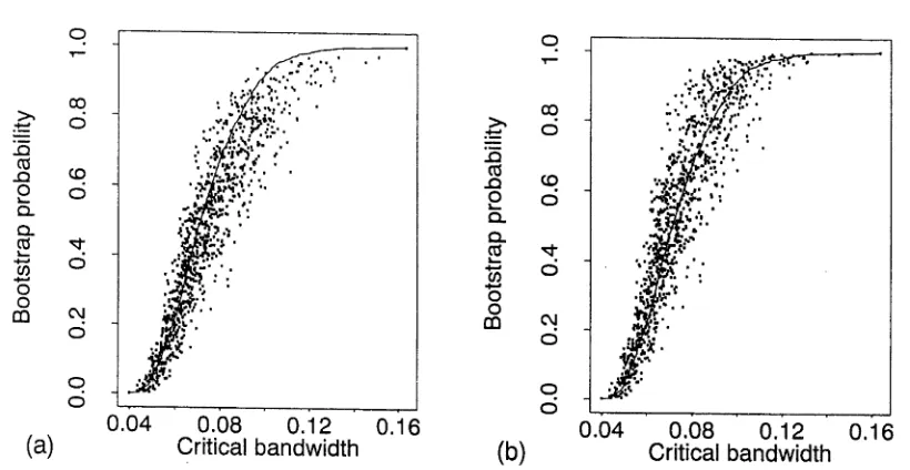
To implement the test we need to have a method of determining when hCT\tj is too large to be consistent with the null hypothesis. Silverman (1981) suggested the use of a smoothed bootstrap technique for assessing significance. Let f cr-lt denote the version of fh obtained by putting h = hcritJ. Conditional on X, let X J , ... , X *

be a resample drawn from the distribution with density / cr,t , and put

f *{x) = {n h ) - ' ± K ( ^ X ' } .

Let h*critj denote the version of hcr\tj in this setting, that is, the infimum of all bandwidths such that /*rit has at most j modes. Silverman (1981) used the bootstrap distribution function

P( h Uj < h ^ d \ x )

to estimate the distribution of hcrity, and one minus the probability (1.4) was used as a p-value.

Hq) that is closest to the data. By closest we mean that it uses the least amount of smoothing among all estimates that satisfy HQ. Since a kernel density estimate is a convolution of the empirical distribution function with the kernel function we can generate independent realisations X* from f CT\t by

X^ = A / ( i ) “I“ h-crit,j^i ? ( B 5 )

where X j ^ are sampled uniformly, with replacement, from X, and e* are independent standard Normal random variates.

Silverman (1986, Section 6.4.1) recommends that rather than resampling from

/ c r i t we should resample from a. rescaled version of it that has the same first two moments as the original data X . It can easily be seen that resamples generated

using the scheme (1.5) will have a variance of a2 + h2v{i^ where a2 is the variance of the original data. It is recommended to use the refinement, suggested by Efron

(1979),

X* = X + ( X / ( j ) - X + h c r i t j f z ) / (1 + ^ c r i t , j / ^ “ ) 1/2 5 ( 1 - 6 )

where X and a 2are the sample mean and variance of X. It will be seen in Chapter 3 that this correction greatly improves performance of the test for finite sized samples.

Silverman (1983) observed that by resampling from / crjt , a density on the bound­ ary of H0 and Hi, the bootstrap probability (1.4) will provide a conservative assess­ ment of the significance of H\. In fact this method is extremely conservative. The simulations of Mammen, Marron and Fisher (1992) and Fisher, Mammen and Mar­ ron (1994) provide numerical evidence of this and Mammen et al. present a very convincing heuristic argument, along with theoretical results on h*crit •, to explain this conservatism. Chapters 2 and 3 of this thesis examine the extent of this con­ servatism and suggest ways of improving the accuracy of the test.

Alternatives to the bootstrap for assessing the significance of the test, for the case of j = 1, are assessing hCTjtJ against a standard family of unimodal distributions (Silverman, 1986, p. 140) or approximations based on the asymptotic distribution of

hcr\i j (Hall and Wood, 1996). Hall and Wood (1996) develop conservative Normal approximations to the asymptotic distribution of hCTjty and argue that these methods are more accurate than the bootstrap method described above since this simple

CHAPTER 1. INTRODUCTION 10 also investigate the related problems of testing for the number of shoulder points of

a density (points where f ( x ) = f i x ) = 0) and the number of points of inflexion (points where f"(x) = 0).

Over the past fifteen years the critical bandwidth test has become the most pop­ ular method for determining the number of modes in a population. In many ways this popularity is due to the test being based on the kernel density estimator. Since the kernel density estimator is the most widely used and understood nonparamet- ric density estimator, after the histogram, the ideas on which the test is based are generally well understood and hence the test is an intuitively appealing one. In ad­

dition, the most important and often most troublesome feature of kernel estimation is the choice of the bandwidth and this problem has been widely studied without an entirely satisfactory solution being found. Jones, Marron and Sheather (1996)

provide a recent survey of bandwidth selection techniques for density estimation. However for the bandwidth test the bandwidth is chosen automatically in a very natural manner, and this makes the test extremely easy to implement.

However, a test that depends on a density estimator will inherit any undesirable properties that estimator might have. In the context of mode testing, the most serious of these properties of a kernel density estimator with a global bandwidth is that these estimators will often have spurious modes in their tails, caused by the sparsity of data towards the edge of the sample. This can result in the test falsely detecting non-existent modes in the tails of a distribution. Another problem is that the test has troubles with densities that are difficult to estimate using a

kernel estimator with a global bandwidth. For example, if a density has a number of modes of widely varying shapes then the test has difficulties detecting the correct

number of modes (Minnotte, 1997).

In Chapter 2 we address the situation of testing for the number of modes over a compact interval, instead of the usual practice of testing for modes over the whole real line. This approach allows us to avoid the problem of detecting spurious modes in the tail of a distribution and it can alleviate other weaknesses of using a global

1.4

T h e D I P t e s t

Hartigan and Hartigan (1985) proposed the DIP statistic as a measure of the multi­ modality of a sample. It is the maximum difference between the empirical distribu­ tion function and the unimodal density that minimises that distance. This statistic has the advantage of being based on the empirical distribution function and does not require the explicit estimation of a density, unlike the procedures of Good and

Gaskins (1980) and Silverman (1981). The DIP is defined by

D(F) = min max \F(x) — G(rc)|,

GCzU x

where U is the class of unimodal functions. The DIP can be used to measure departures from unimodality since D(F) = 0 for F C U and D(F) > 0 for F (fc U.

The DIP test of unimodality of a sample of size n is based on calculating the DIP for the empirical distribution function Fn. Define

p(Fn, F) = max |Fn(z) - F(x)\

X

and observe that the following two inequalities

D(Fn) < D(F) + p{Fn, F)

and

D(F) < D(Fn) +

hold. The Glivenko-Cantelli theorem states that p(Fn, F) —> 0 almost surely, which implies that D(Fn) —> D(F) almost surely. Asymptotically D(Fn) will be zero for samples generated from unimodal distributions and will be positive otherwise.

Therefore a test based on the DIP will asymptotically distinguish any unimodal F

from any multimodal F.

CHAPTER 1. INTRODUCTION 12 In testing the null hypothesis that a distribution is unimodal versus the alter­

native that it is multimodal a method is needed to calculate the significance of the computed DIP. Hartigan and Hartigan (1985) suggest that this could be done by following Silverman (1981) and resampling from the unimodal distribution that is closest to the data; in this case closest means the distribution that minimises the DIP. However they recommend the simpler, but more conservative, option of using

the Uniform distribution as a unimodal, null distribution.

The Uniform is chosen as the reference distribution since Hartigan and Hartigan

conjecture that the DIP statistic D(Fn) is asymptotically largest for the Uniform distribution amongst all unimodal distributions. Using the “least-favourable” uni­ modal distribution to assess significance will result in a conservative test. Unfor­ tunately the DIP is not stochastically larger for the Uniform than for any other unimodal distribution, for all sample sizes n, but they prove two asymptotic results that convincingly support their conjecture.

The first is that, for a sample from the Uniform on (0,1), y/nD(Fn) -> D(B)

in distribution as n —» oo, where B is a standard Brownian bridge. The second is that, for unimodal distributions whose densities decrease exponentially away from the mode, aJ n D ( F n) —» 0 in probability. These results support the conjecture

since they show that \JnD(Fn) is asymptotically positive for the Uniform but is asymptotically zero for a wide class of unimodal distributions.

Hartigan and Hartigan (1985) give the commonly used percentage points of the DIP statistics for samples of a range of sizes, drawn from the Uniform distribution. They also perform some power calculations. Sommer and McNamara (1987) examine the power of the test when the underlying distribution is a known mixture of two Normal distributions.

1.5

Excess mass estim ates and tests

Müller and Sawitzki (1991) propose excess mass estimates as a method for analysing the modality of a distribution. They prefer to think of modes in the statistical terms of being a region where an excess of probability mass is concentrated rather than in the analytical terms of being a local maximum of the density. Their approach is based directly on the empirical distribution function which means that it does not

of modes to be separated from questions concerning their location.

For a distribution with density / the excess mass functional is

E (A) = t [ / ( * ) - A ] + <J*,

which is the amount of probability mass concentrated above a certain level A > 0.

It can be considered to be a measure of the “distinctiveness” of a mode.

E (A) is a sum of contributions Ec(X) = f c [f(x) — A\dx, coming from the connected sets C, where C C {x : f (x) > A}. The connected components of

{x : f ( x) > A} are known as A-clusters and as A increases the A-clusters concentrate on modes. For any A, a distribution with m modes has at most m A-clusters. The excess mass Em(A) for m modes is defined as

m „

Em{A) = sup V / [f(x) - A] d x, (1.7) C l , . . . , C m j — \ 'I Cj (A)

where the supremum is taken over all sequences { C i,... , Cm} of disjoint connected intervals. Equation (1.7) can be written as

m

Em(A )= sup £ {F(C J) - A ||C ,||} , (1.8) C1 ,.•• iCm j — \

where F(C) is the F-measure of C and ||C|| is the length of the interval C.

Given a sample X — { X i,... , X n} drawn from the distribution F we substitute the empirical distribution function Fn for F in (1.8) to obtain the estimator

m

Enm(a) = sup

yy

To test the null hypothesis that / has m — 1 modes against the alternative that it has m modes Müller and Sawitzki (1991) suggest that a large difference

Dnrn{A) Enm(X) l (A),

for some A indicates a violation of the null hypothesis. Hence they recommend the use of

Xnm sup DnmiKA) A > 0

CHAPTER 1. INTRODUCTION 14 Müller and Sawitzki (1991) present an algorithm for finding the components C3

that minimise the sum in equation (1.9), which they call the empirical A-clusters.

The algorithm also computes the excess mass estimate E nm(A). In the absence of flat parts of / the empirical A-clusters consistently estimate the real A-clusters. The empirical A-clusters show the location of mass concentration and plotting them against A can be used as a data analysis tool. This idea is similar to mode tree of

Minnotte and Scott (1993); see Section 1.6.

It is interesting to observe that in the case of testing for two modes versus one mode the excess mass test is identical to Hartigan and Hartigan’s (1985) DIP test.

The excess mass statistic An 2 is equal to twice the DIP statistic. Hence the following discussion of ways of developing a method for accurately assessing the significance of the excess mass statistic obviously also applies to the DIP statistic.

In the previous section we saw that the significance of a calculated DIP statis­ tic is usually determined by reference to the distribution of the DIP calculated for

samples drawn from a Uniform distribution. This choice of the Uniform as a ref­ erence distribution was justified by theoretical results which showed that the DIP was asymptotically larger for the Uniform samples than for samples drawn from unimodal distributions whose densities decrease exponentially away from the mode.

Similarly for the excess mass test, Müller and Sawitzki have shown that for sam­ ples drawn from a Uniform distribution Anm is of exact order Op(n~1/2), and Cheng and Hall (1998) have shown that Anm is of exact order Op(n_3//5) for distributions without any flat parts (see Cheng and Hall (1998) for the precise regularity condi­ tions). Therefore the use of the Uniform as a reference distribution will produce an asymptotically conservative test. In fact, it will be extremely conservative. Since Anm is of a larger exact asymptotic order for the Uniform than for distributions without any flat parts, the use of the Uniform as a reference distribution will result in a test with an asymptotic level of zero for each non-zero value of the nominal level

(Cheng and Hall, 1998). The conservatism of the test results in it having rather low power.

Cheng and Hall (1997, 1998) develop two forms of the test both of which produce

a test that is asymptotically accurate. They concentrate on the case of testing the null hypothesis of unimodality versus the alternative of multimodality. Their approaches exploit the fact that the limiting distribution of Anm, under the null

may be estimated. They prove that n3|/o An2 converges in distribution to cZ as n —» oo, where c = {/(^o)3/ | / //(^o)|}1,/5) is the location of the unique mode of / and Z is a random variable whose distribution does not depend on / .

Their first method requires resampling from a distribution F°, for which the

properties of An2 are similar to those under F if the null hypothesis is true. Since the limiting distribution of An2 depends only on / through the constant c, the only requirement on F° is that it has a unimodal density /° with the same value of c

as / . In their implementation Cheng and Hall use kernel methods to estimate / and /" . Notice that the estimates / and f " require different amounts of smoothing. They use the respective asymptotically optimal global bandwidths for a Normal

N (0, s2) distribution, where s2 is the sample variance. Once c has been estimated by c = { f ( xo) / f " ( x 0)}]/5, where xq is the location of the largest mode of / , they

choose f ° to be a density from a family of Beta, Normal and Student-t densities with a value of c equal to c.

The procedure is to draw a resample X* = {A *,... , X*} from the distribution F° and compute A*2, the version of An2 for the resampled data X*. To construct a test at level a, use Monte Carlo methods to compute the critical point za defined by

Pf o(A ;2 > zQ I X) = a,

and reject the null hypothesis that / is unimodal if An2 > za. Under mild regularity conditions, including that c is a consistent estimate of c under the null hypothesis, the test has asymptotically correct level (Cheng and Hall, 1998).

Cheng and Hall also show how their method can be applied to the more general problem of testing the null hypothesis that / has m modes against the alternative that / has m -f 1 modes, for m > 2. They conduct a simulation study that demon­ strates that their test has very good level accuracy and greatly improved power. They compare their method with Silverman’s (1981) critical bandwidth test and find that their method generally has better level accuracy under the null hypothesis

and greater power under the alternative. It also avoids the problems of finding spu­ rious modes in the tails of a distribution that the bandwidth test often encounters.

Cheng and Hall (1997) consider a second method of calibrating the test. Rather

CHAPTER 1. INTRODUCTION 16 of testing the null hypothesis that / has two or more modes. Cheng and Hall’s

(1997) simulation study also suggests that the method that involves explicitly esti­ mating c generally outperforms this double bootstrap technique. The method that we develop in Chapter 2 for calibrating Silverman’s bandwidth test is closely related to this double bootstrap procedure for the excess mass test.

The most attractive feature of DIP and excess mass tests is that they are based directly on the empirical distribution function and do not require a density estimate to be calculated. A test that relies on a density estimate can be no more effective than the estimate on which it depends, since the test will inherit any undesirable

properties that the estimator might have. We saw in Section 1.3 that the critical bandwidth test has problems with falsely detecting modes in the tails of a distri­ bution and encounters difficulties with multimodal distributions whose modes are of widely varying shapes and sizes. These problems arise because the bandwidth test is based on a kernel density estimator with a global bandwidth, and a band­ width that produces a good estimate in one region does not necessarily produce a good estimate in other regions. Another advantage to directly using the empirical

distribution function to assess modality is that it does not require the specification of a bin width (e.g. Cox, 1966) or a smoothing parameter (e.g. Good and Gaskins,

1980).

However, the properties of the excess mass test that protect it from falsely iden­ tifying spurious modes in the tails can also make it insensitive to the presence of

minor modes. The test is based on the amount of probability mass above a level A. If the height of a minor mode is below the height of the trough between two major modes then A will be chosen to be above the height of the minor mode and it will

make no contribution to the excess mass statistic. Consequently the test will not be able to detect the presence of this smaller mode.

in spite of the difficulties associated with tests that rely on density estimation, the critical bandwidth test has proved to be more popular with practitioners than

excess mass tests. This is partly due to the intuitive appeal of a method that depends on a simple density estimate, that can be plotted and examined, rather than a test

1.6

T h e m ode tre e an d m o d e ex isten ce te s t

Silverman’s technique tests for the unimodality, bimodality or multimodality of a data set as a whole and is based on a kernel density estimate with a global bandwidth. Minnotte and Scott (1993) and Minnotte (1997) suggest a mode existence technique which tests the significance of each mode individually, using a different bandwidth for each potential mode. This approach can be advantageous since we are often interested in knowing whether the appearance of a concentration of data points in a sample represents a true mode of an underlying population, rather than knowing

precisely how many modes there are in a population. Using different bandwidths for each potential mode allows a degree of local adaptivity which can be quite important, especially when modes occur on peaks of varying sizes.

The mode existence test relies on an exploratory, graphical tool developed by Minnotte and Scott (1993) which they called the mode tree. The mode tree is a graph which plots the mode locations for a kernel density estimate against the bandwidth at which the density estimate with those modes is calculated. It provides a simple yet informative format for displaying how modes split and new modes appear, as

the bandwidth decreases and for which bandwidths these splits occur. Minnotte and Scott (1993) recommended the use of the Normal kernel because the monotonicity of the number of modes, as a function of the bandwidth, ensures that all modes found at a given level of h remain as h decreases.

Other features of density estimates besides the location of the modes can be added to the mode tree. These include the location of antimodes and points of

inflection, and intervals which contain bumps could be shaded. An interval whose length is proportional to the size of the mode could also be shaded. Minnotte and Scott define the size of mode j, for a bandwidth h, as

where a3 and b3 are the locations of the left and right antimodes surrounding mode

j. The quantity Mj is the probability mass of the mode above the higher of the two surrounding antimodes. In a sense Mj is the single mode equivalent to Müller and Sawitzki’s (1991) excess mode functional, evaluated at the height of the the higher

CHAPTER 1. INTRODUCTION 18 function.

Minnotte and Scott (1993) and Minnotte (1997) propose using Mj as a test statistic to test the null hypothesis that mode j is an artefact of the sample against the alternative that mode j is a true feature of the population. Minnotte (1997) investigated the theoretical properties of Mj. He showed that Mj converges in probability to zero when the null hypothesis is true. When the alternative is true it converges to its true population value

where a and b are the locations of the left and right antimodes surrounding the mode. See the original paper for the exact rates of convergence and other technical details. These results show that the use of M0 as a test statistic produces a consistent test.

In implementing the test it is necessary to choose a bandwidth at which to compute Mj(h). Minnotte (1997) shows that Mj{h) is a non-increasing function of h and suggests choosing h such that Mj(h) is as large as possible, in order to produce a test with maximum power. This is achieved by choosing h as small as possible without the mode splitting into two new modes.

Following Silverman (1981), Minnotte and Scott (1993) suggest a resampling ap­ proach to assess the significance of Mj. They resample from f-h but with the mode that is being tested and at least one of the adjacent antimodes being replaced with a flat section. This approach can be viewed as being a single mode version of Har- tigan and Hartigan (1985) and Müller and Sawitzki’s (1991) approach to assessing the significance of their statistics based on comparison of properties with samples of Uniform random variables; see Section 1.5 for a discussion of these methods. These techniques are known to be even more conservative than Silverman’s (1981)

bootstrap technique. The p-values and power results reported in Minnotte’s (1997) simulation study support this view.

The simulation study and Minnotte and Scott’s (1993) application of the test to the stamp data (from Izenman and Sommer, 1988) show that when the modes

occur on peaks of varying sizes the local, adaptive approach of their test has distinct advantages over the global approach of Silverman’s test. In Section 2.4 and Chapter 4 we show that some of the problems associated with the non-adaptivity of using a global bandwidth can be alleviated by testing for the number of modes over a compact interval, which is a subset of the support of the density, rather than over

the whole real line.

1.7

M o d e te s tin g in h ig h er d im en sio n s

In the earlier sections of this chapter we have considered methods for assessing the

modality of univariate populations. In this section we shall conduct a brief survey of methods that have been developed for investigating the modality of multivariate

populations. Some of these methods are generalisations of univariate approaches, such as the work of Hartigan (1987) and Polonik (1995a) on multivariate excess mass estimates and Hartigan’s (1988) adaption of his univariate DIP statistic into the multivariate SPAN statistic. Others, such as Hartigan and Mohanty’s (1992) RUNT test and Rozäl and Hartigan’s (1994) MAP test, are novel approaches that can be applied to data of all dimensions but are designed particularly with higher dimensional data in mind.

Hartigan (1987) developed an excess mass approach for a density in two dimen­ sions, independently of Müller and Sawitzki’s (1987) work in one dimension. He

examined the problem of estimating a convex density contour using excess mass to estimate the amount of probability mass above a given contour level. Hartigan used his method to develop a test for bimodality, with the test statistic being an estimate of the excess probability located in a secondary mode.

Polonik (1995a) examined estimating excess mass over a class of subsets of

d-dimensional Euclidean space, and used this estimate to develop a generalisation of the excess mass statistic for multimodality (Müller and Sawitzki, 1991), for

d-dimensional populations. Polonik (1995b) looked at the closely related problem of estimating a d-dimensional density under shape restrictions on the density contour clusters. By choosing these shape restrictions appropriately it is possible to model various features of the data, including multimodality.

Hartigan (1988) developed the SPAN test as a multidimensional generalisation of the DIP test. The SPAN test uses distribution functions defined on rooted min­ imal spanning trees instead of the usual multivariate distributions. The minimum

CHAPTER 1. INTRODUCTION 20 the maximum difference between the EDF and it closest unimodal approximant.

Given a sample X \ , ... , An, the empirical distribution Pn gives probability 1/n to each sample point. The SPAN for this distribution is defined to be

SPAN(Pn) = min SPAN(Fnr) ,

r

that is, the minimum distance between the EDF and its closest unimodal approxi­

mant, minimised over all choices of the root node. The computation of the SPAN statistic is quite involved and the algorithm takes between n2 and n3 steps.

Hartigan conjectures that if the sample is from a continuous unimodal density / then SPAN(Pn) —> 0, as n —> oo, and that when / is not unimodal, SPAN(Pn)

converges in distribution to a positive random variable. These results have been

proven for the one-dimensional DIP statistic. The paper gives the 95% point of the SPAN distribution for up to 5 dimensions, based on samples drawn from a Uniform distribution on the sphere.

Hartigan and Mohanty (1992) propose the RUNT statistic as a more simply computed alternative to the SPAN statistic. It uses single linkage clustering for detecting the presence of multimodality in populations. Single linkage clusters on a set of points are the maximal connected sets in a graph constructed by linking all points within a given threshold distance of each other. The complete set of single linkage clusters is obtained from all graphs constructed using different threshold distances. As the threshold distance is decreased each cluster divides into two or

more subclusters until each cluster consists of a single point. For each single linkage cluster the runt size is the number of points in its smallest subcluster. The RUNT statistic is the maximum runt size over all threshold distances. Large values of the RUNT suggest multimodality.

Justification of the test is based on the asymptotics of single linkage clusters; see Hartigan (1981). It there are at least two modes in the population density, then asymptotically, just one of the single linkage clusters will split into two clusters of points, one about each of the modes. The smaller of these two clusters will be the runt. If there is a single mode, then asymptotically, each cluster will divide into two clusters, the smaller of which will contain very few points. Therefore we would expect

a larger number of points in the runt when the distribution is multimodal and thus a large value of the RUNT statistic should indicate the presence of multimodality.

simulations show that the test has highest power for 3, 4 and 5 dimensions.

Rozäl and Hartigan (1994) introduced a test based on minimal constrained span­ ning trees. They define a Minimal Ascending Path Spanning Tree (MAPST) which is the minimal spanning tree whose link lengths are non-increasing on the path to the root node, starting from any link. MAPSTs with more than one root are also defined to accommodate the possibility of multimodality. A multiple root MAPST is a minimal spanning tree constrained so that starting from any link there is a path

to one of the root nodes satisfying the ascending path property. Rozäl and Hartigan present algorithms for finding MAPSTs.

Nearest neighbour density estimates are used to develop a test statistic. Let

X i , ... , X n £ IZd be a sample from a density / with an unknown number of modes. Let rk(x) be the Euclidean distance from x to the k-th nearest point. If cd is the volume of the unit sphere in lZd, then Vk(x) = is the d-dimensional volume of the d-dimensional sphere Sk(x) of radius rk(x) centred at x. Of the n

sample points, it is expected that about nf ( x) Vk(x) fall inside Sk(x). Equating this expected number with the number k actually observed gives the nearest neighbour estimate of / at x,

The d-th root of the density estimate is inversely proportional to the distance of the k-th nearest point from x. Thus the density is highest where the points are closest together, indicating existence and location of modes. Taking logarithms of

both sides of (1.10) gives

For each point in the sample , X n let Tu(X{) (U for unimodal) be a MAPST with a single root at Xi. Let TB{Xil, X l2) (B for bimodal) be a MAPST with roots at X lx and X l2. Let px,(Xj) be the length of the link from X 3 to the next mode vxi(Xj) in the direction towards the root in TB{Xi). Define the functions

Lu{Xi) and L B( Xll, X l2), which are the sum of the logarithms of the lengths of the links in Tu(Xi) and TB(Xtl, X i2) respectively, by

f (Xs) —--- =

---nVk{x) ncdrk(x)d ' (1.10)

(1.11)

indicating that log f (x) is linear in the minus log distance to the /c-th nearest point.

CHAPTER 1. INTRODUCTION 22 and

L B( Xil, X i2) = lo g\ l™lni2 Pxi(X i ) \ + l o g D { X il, X i2),

j ^ i \ , 12 ^ 1 2

where D ( X l}, X l2) is the distance between the subclusters belonging to the roots

X h and X i2 in TB( Xh , X i2).

Equation (1.11) suggests that — log p x ^ X j ) is roughly proportional to the log density at X r Thus, when / is unimodal —Lu(Xi) should be roughly proportional to the log-likelihood log f ( Xj ) . When / is bimodal some of the distances

PXi{Xj) will be substantially larger than the nearest neighbour distances. Then

Lu(Xi) should be larger than minus the log-likelihood. However, under bimodality

— LB(Xil i Xi 2) will be close to the log-likelihood. The MAP statistic for bimodality is defined by

MAP = min Lu(Xi) - min L B{Xn , X l2). i hyi2

The quantities Ly and Lb are minimised when the roots are chosen to be close

to the modes of / . Under unimodality, except for small links near the roots, the unimodal and bimodal trees will be nearly identical and the value of the MAP will be near zero. If / is bimodal the root of the minimal unimodal tree Tu will be near one of the modes and the links of Tu that connect points belonging to the other mode will be considerably longer than those links in the minimal bimodal tree TB

that, connect those points into TB. There will be a considerable difference between the minima of Lu and of LB\ the MAP will be bounded away from zero.

The MAP test can be extended to testing the null hypothesis that / has two or more modes. The significance of the test can be determined by comparing values from samples taken from a reference distribution or by using a resampling method proposed by Rozal and Hartigan (1994).

1.8

F in ite m ix tu re d is trib u tio n s

In the introduction to this chapter we argued that if the density connected with

Finite mixture densities have the form

k

f ( x) = E K jfii* \0j) . (1-12)

3=1

-_

where 7Tj > 0 for j = 1 ,... , fc, 71 j = 1 and /1, • • • , /jt are probability density functions. The parameters 7^ , . . . , 7rfc are usually known as the mixing proportions and /1, . . . , /fc are known as the component densities.

While the presence of multimodality is indicative of a mixture distribution not all mixtures are multimodal. For example, an equal mixture of two Normal distributions

with a common variance will only be bimodal if the distance between the means of the two Normals is greater than twice the standard deviation of the component

densities. When the components of a mixture are sufficiently well separated the mixture density will be multimodal. Heavily overlapping mixture components will tend to induce inflection points and skewness in the mixture densities, rather than multimodality.

Hence knowing the number of modes in a density will provide a lower bound on the number of components in a mixture. We shall see later in this section that determining the number of components in a mixture can be very awkward. In addition to this awkwardness, the use of mixtures generally requires the assumption of a parametric model for each of the components. The assessment of the number of components in a mixture can be heavily influenced by the validity of the particular parametric model. For example, if it is assumed that the components of a mixture are Normal but they are actually skewed then each component might require a

mixture of two or more Normals to adequately describe it. This would result in the assessment of the number of components, based on the parametric model, to overestimate the number of homogeneous subpopulations contained in a population.

Finite mixture distributions have a wide variety of applications and have been extensively studied. Three monographs on the topic are Everitt and Hand (1981),

Titterington, Smith and Makov (1985) and McLachlan and Basford (1988).

CHAPTER 1. INTRODUCTION 24 as

x — [1j

(1.13)

where 4> is the standard Normal density function and fij and oy are the mean and standard deviation of the jth component, respectively.

The class of mixture distributions is an extremely rich one and if k and are unrestricted then any continuous density can be arbitrarily closely approximated by

a Normal mixture. In fact, the Normal kernel density estimator (see Section 1.3) is a Normal mixture. This can be seen by setting k = n, 7iy = 1/n, fij = X 3 and oy = h

in equation (1.13). In practice there need to be some restrictions introduced in order for models of form (1.13) to be able to usefully estimate densities. For example, for kernel density estimates the bandwidth h is the only arbitrary parameter.

If we wish to estimate a density using a Normal mixture, based on a sample

X i , . . . , X n, there are two problems that need to be considered. Firstly, we need to determine k, the number of components in the mixture, and secondly, given k,

we need to estimate the parameters 7iy, and oy associated with each component. Neither of these two problems is as straightforward as it first appears. We shall consider the second problem first. The most common method for determining the parameters for a parametric model is maximum likelihood. For a Normal mixture the likelihood is

The maximum likelihood estimates 7iy, py and by of the parameters are those values that maximise (1.14). However the likelihood surface is littered with singularities.

To see this, put = X\, and note that L —> oo as o\ —» 0. In spite of these singularities, a strongly consistent maximum likelihood estimator can be obtained (Titterington et al, 1985, Section 4.3.3) as long as we keep away from singularities on the boundary of the parameter space.

Since the maximiser of (1.14) has no explicit solution, it is necessary to use iterative, numerical methods to obtain maximum likelihood estimates. The EM al­ gorithm (Dempster, Laird and Rubin, 1977) has become a popular method because

of its ease of implementation, low storage requirements and robustness against poor initial values; see McLachlan and Basford (1988, Section 1.6). Hathaway (1985,

1986) developed a constrained version of the EM algorithm that prevents conver­ gence to singularities. However in practice the likelihood surface can have many local maxima particularly when there is a large number of parameters to be fitted relative to the size of the data set. While Hathaway’s algorithm reduces the chance of convergence to a local maximum, rather than the global one, the number of local

maxima can make maximum likelihood estimation difficult. Other approaches used to avoid these problems include imposing the condition 0\ = <72 = • • • = Gk or using

minimum distance estimation based on distribution functions (Titterington et al., 1985, Section 4.5).

The other problem is determining k, the number of components in a mixture. This is a very difficult problem and no clear statistical procedure has been developed. The obvious generalised likelihood ratio test does not yield the usual asymptotic chi- squared distribution under the null. Consider testing the nested hypotheses

The usual asymptotics do not apply since the regularity conditions on which they rely (see Cox and Hinkley, 1974, p. 281) are violated by the parameters of the null hypothesis being located on the boundary of the parameter space of the alternative

hypothesis. In fact, rather than converging to a chi-squared distribution, Hartigan (1985) has shown that the likelihood ratio converges to infinity at a very slow rate.

McLachlan (1987) has used the bootstrap to estimate the null distribution of the likelihood ratio test but this test is very computationally demanding and, in practice,

lacks power because under the null the distribution of the test statistic has a long right tail (Roeder, 1994).

An alternative to formal testing procedures for determining the number of com­ ponents in a mixture is the use of diagnostic graphical tools. These include the use

CHAPTER 1. INTRODUCTION 26 developed a graphical tool and a formal testing procedure based on this result. Un­ der the null hypothesis that k = 1, the proposed diagnostic can be approximated by a stationary Gaussian process while, under the alternative hypothesis, the compo­ nents of the mixture will manifest themselves as modes in the diagnostic plot. The graphical tool involves examining a plot of the fluctuations in the process and com­

paring the amplitude of the fluctuations with asymptotic confidence bands derived under the null. The formal test borrows critical smoothing ideas from Silverman (1981) and is based on the amount of smoothing required to suppress the deviations from the stationary Gaussian process.

Roeder (1990) proposed a semiparametric density estimation technique that en­ tails choosing a Normal mixture that maximises a function based on sample spacings. The estimation technique relies on the selection of a smoothing parameter. Roeder suggested using cross-validation to choose the smoothing parameter to obtain a

point estimate of the density and provided a means of determining a confidence set of plausible densities. The confidence set consisted of the set of Normal mixtures fitted using a range of smoothing parameters. The boundaries of the smoothing parameter are determined by inverting a distribution-free goodness-of-fit statistic. By considering a range of values for the smoothing parameter and the accompanying confidence set of densities, ranging from smooth to rough, we can obtain a handle on the number of modes in the density.

C a lib ra tin g S ilv e rm a n ’s te s t

2.1

In tro d u ctio n

In this chapter we propose methods for overcoming some of the weaknesses of Sil­ verman’s (1981) critical bandwidth test for testing the null hypothesis that a dis­ tribution has j modes versus the alternative that it has j + 1 or more modes. In Section 1.3 we identified two main difficulties with Silverman’s test. The first of these problems was that the bootstrap part of the test does not consistently esti­ mate the distribution of the critical bandwidth hCTjt , the test statistic. This results in a very conservative test. We propose a version of the test, in the important case

j = 1 that produces a test with asymptotically correct level and which has greater power than the standard test. Bootstrap calibration techniques were first discussed by Hall (1986, 1987) and Loh (1987, 1991) in the context of improving the coverage

accuracy of bootstrap confidence intervals.

The second problem was that the testing problem is often made more difficult by spurious modes arising from outlying data values. We suggest conducting the test over a compact interval rather than over the whole line. We study this modified

version of the test and show that, asymptotically, this form of the test has correct level under quite general conditions.

The numerical results related to the work described in this chapter can be found

in Chapter 3. In Chapter 4 we apply the various forms of the test to real data sets.