Dimensionality Reduction Methods: The Comparison Of Speed And Accuracy

(1)

Dimensionality Reduction

Methods: The Comparison

of Speed and Accuracy

ITC 1/47

Journal of Information Technology and Control

Vol. 47 / No. 1 / 2018 pp. 151-160

DOI 10.5755/j01.itc.47.1.18813 © Kaunas University of Technology

Dimensionality Reduction Methods: The Comparison of Speed and Accuracy

Received 2017/08/11 Accepted after revision 2018/01/25

http://dx.doi.org/10.5755/j01.itc.47.1.18813

Jelena Zubova, Olga Kurasova

Vilnius University, Institute of Mathematics and Informatics, Akademijos str. 4, LT-08663 Vilnius, Lithuania, e-mails: [email protected], [email protected]

Marius Liutvinavičius

Vilnius University, Kaunas Faculty, Muitinės str. 8, LT-44280 Kaunas, e-mail: [email protected]

Corresponding author: [email protected]

This research focuses on big data visualization that is based on dimensionality reduction methods. We propose a multi-level method for data clustering and visualization. It divides the whole data mining process into sep-arate steps and applies particular dimensionality reduction method considering to analyzed data volume and type. The methods are selected according to their speed and accuracy. Therefore, we present a comparison of the selected methods according to these two criteria. Three groups of datasets containing different kind of data are used for methods evaluation. The factors that influence speed or accuracy are determined. The rank of in-vestigated methods based on research results is presented in this paper.

KEYWORDS:big data, dimensionality reduction, data visualization.

1. Introduction

Big data analytics is the process of investigating big data to uncover hidden and useful information for better decisions. It involves visual presentation of data that enables to see hidden relations between ob-jects which cannot be detected using conventional data analysis methods [14].

(2)

Information Technology and Control 2018/1/47 152

information as possible [6].

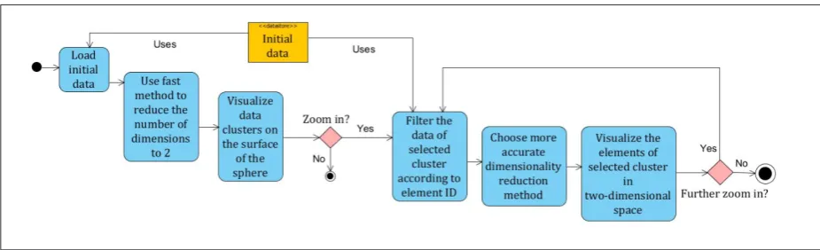
We propose a method which divides the data mining process into separate steps. At each stage, a particular dimensionality reduction and visualization method is applied considering to data volume and type. The methods are selected according to their speed and ac-curacy. Therefore, in the second section of this paper we present the comparison of selected dimensionali-ty reduction methods.

When data are clustered and visualized, there is a possibility to see the parameters of each data group. The further analysis is performed only for the select-ed data cluster.

At the initial stage, the accuracy of method is not so important, so the fastest visualization method can be used. For the following dimensionality reduction steps, the demand for accuracy gradually increases. This requires using more accurate, but possibly slow-er methods. During each step, the selected data clus-ter is divided into smaller sets. At the end, the most accurate method processes the data. It would require too much resources at the beginning of dimension-ality reduction, but at the end the data set is small enough to be processed in the most accurate way. Most often in scientific literature there are just qual-itative comparisons of different dimensionality re-duction methods [2], [12], [11]. In some papers [6], [5], we can also find speed or accuracy comparisons of selected methods. The review of such researches leads to insight that some methods are faster, but less accurate and that other ones have opposite character-istics. However, there is a lack of general quantitative

research of most popular methods that would com-pare both speed and accuracy.

Therefore, in this paper we investigate these well-known methods: Multidimensional Scaling (MDS), Principal Component Analysis (PCA), Independent Component Analysis (ICA), Principal Curves, Local-ly Linear Embedding (LLE), and Isometric Mapping (Isomap).

2. A Review of Dimensionality

Reduction Methods

A brief summary of the most popular dimensional-ity reduction methods is presented in this section. It is based on researches previously made by Fodor [2], Mizuta [7], Sorzano et. al. [12]. According to them, much of the data are highly redundant and can be ef-ficiently brought down to a much smaller number of variables without a significant loss of information. Multidimensional scaling (MDS)

Given n items in a d-dimensional space and an n x n matrix of proximity measures among the data items, MDS produces a k-dimensional, k ≤ d, representation of the items such that the distances among the points in the new space reflect the proximities in the data [2]. In this research, we use mds() function from R pack-age ‘smacof’ [11]. It solves the stress target function for symmetric dissimiliarities by means of the major-ization approach (SMACOF) and reports the Stress-1 value (normalized).

Figure 1

A Multi-level method for big data visualisation

2

method processes the data. It would require too much

resources at the beginning of dimensionality reduction, but at the end the data set is small enough to be processed in the most accurate way.

Figure 1. A Multi-level method for big data visualisation

Most often in scientific literature there are just qualitative comparisons of different dimensionality reduction methods Error! Reference source not found., Error! Reference source not found., Error! Reference source not found.. In some papers Error! Reference source not found., Error! Reference source not found., we can also find speed or accuracy comparisons of selected methods. The review of such researches leads to insight that some methods are faster, but less accurate and that other ones have opposite characteristics. However, there is a lack of general quantitative research of most popular methods that would compare both speed and accuracy.

Therefore, in this paper we investigate these well-known methods: Multidimensional Scaling (MDS), Principal Component Analysis (PCA), Independent Component Analysis (ICA), Principal Curves, Locally Linear Embedding (LLE), and Isometric Mapping (Isomap).

2. A Review of Dimensionality Reduction Methods

A brief summary of the most popular dimensionality reduction methods is presented in this section. It is based on researches previously made by Fodor [2], Mizuta [7], Sorzano et. al. [12]. According to them, much of the data are highly redundant and can be efficiently brought down to a much smaller number of variables without a significant loss of information. Multidimensional scaling (MDS)

Given n items in a d-dimensional space and an n x n matrix of proximity measures among the data items, MDS produces a k-dimensional, k ≤ d, representation of the items such that the distances among the points in the new space reflect the proximities in the data Error! Reference source not found..

In this research, we use mds() function from R package ‘smacof’ [11]. It solves the stress target function for symmetric dissimiliarities by means of

the majorization approach (SMACOF) and reports the Stress-1 value (normalized).

This function allows for fitting three basic types of MDS: ratio MDS (used in our case), interval MDS (polynomial transformation), ordinal MDS (also known as nonmetric MDS) Error! Reference source not found..

Principal components analysis (PCA)

PCA is by far one of the most popular algorithms for dimensionality reduction Error! Reference source not found.. It finds components that make projections uncorrelated by selecting the highest eigenvalues of the covariance matrix and maximizes retained variance Error! Reference source not found.. PCA finds the principal components of the data, which correspond to the components along which there is the most variation Error! Reference source not found.. Independent component analysis (ICA)

ICA is a higher-order method that seeks linear projections, not necessarily orthogonal to each other, that are as nearly statistically independent as possible. While PCA seeks uncorrelated variables, ICA seeks independent variables Error! Reference source not found.. It should be noted that statistical independence is a much stronger condition than uncorrelatedness.

Principal curves, surfaces and manifolds

(3)

This function allows for fitting three basic types of MDS: ratio MDS (used in our case), interval MDS (polynomial transformation), ordinal MDS (also known as nonmetric MDS) [10].

Principal components analysis (PCA)

PCA is by far one of the most popular algorithms for di-mensionality reduction [12]. It finds components that make projections uncorrelated by selecting the highest eigenvalues of the covariance matrix and maximizes retained variance [1]. PCA finds the principal compo-nents of the data, which correspond to the compocompo-nents along which there is the most variation [6].

Independent component analysis (ICA)

ICA is a higher-order method that seeks linear projec-tions, not necessarily orthogonal to each other, that are as nearly statistically independent as possible. While PCA seeks uncorrelated variables, ICA seeks independent variables [2]. It should be noted that sta-tistical independence is a much stronger condition than uncorrelatedness.

Principal curves, surfaces and manifolds

In situations where initial data have some curved structure methods like PCA do not work well. In such cases, approximating the curve by a straight line will not perform a good approximation of the original data. For such data type, the solution is to use principal curves, surfaces and manifolds [12]. Curve fitting to data is an important method for data analysis. When we obtain a fitting curve for data, the dimension of the data is nonlinearly reduced to one dimension [7]. Locally linear embedding (LLE)

LLE method is used to learn manifolds close to the data and project them onto them. For each item, it looks for the K‐nearest neighbours and produces a set of weights for its approximation. This optimization is performed simultaneously for all items. Once the weights have been determined, it looks for points of lower dimension. The new points are reconstructed from its neighbours in the same way (with the same weights) as the items they represent [2].

Isometric mapping (Isomap)

If the distances between objectsare measured as

geo-manifold is the one measured along the geo-manifold it-self; in practical terms, it is computed as the shortest path in a neighborhood graph connecting each obser-vation to its K‐nearest neighbors [2].

3. Research Methodology

The main goal of this research is to compare the speed and accuracy of the selected methods of visualization based on dimensionality reduction. R was chosen as a basis for analysis, because there are various open source packages that enable to execute and evaluate different dimensionality reduction methods. RStudio environment was used to perform the tasks.

3.1 Data

Three groups of different kinds of datasets were cre-ated for testing purposes.

Randomly generated nonclustered data

First of all, 50 different datasets containing randomly generated numbers were created with R function sam-ple(). The number of columns is from 10 to 50. The num-ber of items is from 1 000 to 10 000. Thus the smallest dataset is 1 000x10 and the largest one is 10 000x50. Randomly generated clustered data

The second group contains 25 datasets of clustered data. The function genRandomClust from R pack-age ‘clusterGeneration’was used to generate cluster datasets with specified degree of separation [8]. Each dataset has four clusters. The number of columns is from 10 to 50. The number of items is from 1 000 to 9 000. The smallest dataset is 1 000x10 and the largest one is 9 000x50.

Real financial data

The third group contains 20 datasets of real financial data – stock ratios from finviz.com [13]. In total, there is information about 7 000 companies. Each company is described by 50 parameters, which can be grouped into six categories: overview (price, volume, etc.), fi-nancial (ROI, ROA, etc.), valuation (EPS, P/E, etc.), performance (price changes, volatility, recommenda-tions), technical (Beta, SMA, etc.), ownership.

(4)

7 000x50. In all cases of our research, the initial num-ber of dimensions is reduced to two.

3.2 The Evaluation Criteria

We use two main criteria to compare different methods:

_ Speed. It is measured as execution time of

dimensionality reduction process.

_ Accuracy. We use three different measures to

evaluate the accuracy:

Stress – the measure got by solving the square loss function of MDS method. We used R function mds() from package ‘smacof’ to find the stress value. Spearman coefficient (The Spearman’s Rank Cor-relation Coefficient). It is a statistical measure used to discover the strength of a link between two sets of data [3].

This ratio uses the ranks of variables instead of their values. Possible values range from -1 (strong nega-tive relation) to 1 (strong posinega-tive relation). If ratio is equal to zero, this means there is no statistical link between datasets. To calculate this ratio, R function cor() with method “spearman” was used.

Shannon entropy. We used R function entropy from package ‘entropy’ that estimates the Shannon entro-py H of the random variable Y from the corresponding observed items [9], [4].

This estimator shows how accurate the projection got by using particular dimensionality reduction method retains the initial amount of information. A lesser val-ue of this measure means better accuracy.

4. Research Results

The results of speed and accuracy comparison for each group of data are presented in this section. At the end, the overall comparison is made.

4.1 Randomly Generated Nonclustered Data In the first case, randomly generated nonclustered datasets are used for investigation.

The speed of methods

As results show, MDS (smacof), Isomap and LLE methods have the same characteristics:

_ When the number of instances increases, the execution time also increases.

_ The initial amount of dimensions does not have

significant effect on the time of execution.

Fig. 2 shows the execution time of MDS (smacof) method for datasets that contain ten columns, but dif-fer in number of rows. The charts of execution time for the datasets having more columns look the same, because this factor has no influence. However, Iso-map is much slower (this can be seen in Fig. 6).

Figure 2

Execution time of MDS (smacof) method

4

because this factor has no influence. However, Isomap is much slower (this can be seen in Fig. 6).

Figure 2. Execution time of MDS (smacof) method For PCA, the execution time increases just slightly in both cases: when the number of rows increases and when the number of columns increases (Fig. 3):

Figure 3. Execution time of PCA

The execution time of ICA is similar to PCA. Only Principal curves distinguish by regular increase of execution time in both cases (when the number of dimensions and items increase) (Fig. 4).

In Fig. 6, the execution times of tested methods are compared. The number of items is from 1 000 to 10 000. The initial number of dimensions does not have significant influence for any method, so only one case with 40 dimensions is presented.

Figure 5. A Comparison of execution times The accuracy of methods

For all the investigated methods, we found that the same rules apply:

 When the number of items increases, the accuracy does not change.

 When the number of initial dimensions increases, it leads to worse accuracy.

This was confirmed by all measures. However, the level of accuracy reduction is not the same for different methods. Figures 7 and 8 compare the accuracy of all analysed methods. As the number of instances does not make significant influence, we show only the cases with 7 000 items.

In all cases with different number of initial dimensions, the results are similar. Therefore, we present only two of them: 20 dimensions and 40 dimensions.

Figure 6. A Comparison of execution times For PCA, the execution time increases just slightly in

both cases: when the number of rows increases and when the number of columns increases (Fig. 3).

Figure 3

Execution time of PCA

4 because this factor has no influence. However, Isomap is much slower (this can be seen in Fig. 6).

Figure 2. Execution time of MDS (smacof) method

For PCA, the execution time increases just slightly in both cases: when the number of rows increases and when the number of columns increases (Fig. 3):

Figure 5. A Comparison of execution times

The accuracy of methods

(5)

155 Information Technology and Control 2018/1/47

Figure 4

Execution time of Principal curves

4 is much slower (this can be seen in Fig. 6).

Figure 5

A Comparison of execution times

4 because this factor has no influence. However, Isomap is much slower (this can be seen in Fig. 6).

 When the number of items increases, the accuracy

does not change.

 When the number of initial dimensions increases,

it leads to worse accuracy.

It should be noted that LLE could not process the datasets with more than 9 000 rows, Isomap could not

process more than 8 000 rows and for MDS (smacof) the limit was 7 000 rows. This was due to the lack of RAM. In Fig. 5, the speed of methods is presented in a logarithmic scale. PCA and ICA are the fastest. Prin-cipal curves, MDS and LLE are much slower. Howev-er, Isomap is the slowest (its execution time is signifi-cantly longer than that of others).

4 Figure 3. Execution time of PCA

Figure 4. Execution time of Principal curves

It should be noted that LLE could not process the datasets with more than 9 000 rows, Isomap could not process more than 8 000 rows and for MDS (smacof) the limit was 7 000 rows. This was due to the lack of RAM. In Fig. 5, the speed of methods is presented in a logarithmic scale. PCA and ICA are the fastest. Principal curves, MDS and LLE are much slower. However, Isomap is the slowest (its execution time is significantly longer than that of others).

• When the number of items increases, the accuracy does not change.

• When the number of initial dimensions increases, it leads to worse accuracy.

Figure 7. A Comparison of the accuracy measures

Figure 6. A Comparison of execution times Figure 6

_ When the number of items increases, the accuracy

does not change.

_ When the number of initial dimensions increases,

This was confirmed by all measures. However, the level of accuracy reduction is not the same for differ-ent methods. Figures 7 and 8 compare the accuracy of all analysed methods. As the number of instances

Figure 7

(6)

Figure 9

A Comparison of methods by speed and accuracy

5 Figure 8. A Comparison of the accuracy measures

The results show that PCA and MDS were the most accurate with our datasets. LLE showed the worst accuracy.

The rank of methods

Fig. 9 summarizes the results of nonclustered data case. We ranked all investigated methods by their speed and accuracy (“6” means the highest score and “1” stands for the worst score).

Figure 9. A Comparison of methods by speed and accuracy

PCA and ICA are the fastest methods. MDS is the most accurate, but slower. Principal curves showed moderate results. The results of LLE and Isomap are the worst. Even though Isomap is significantly slower, its accuracy in some cases can be the best.

4.2 Randomly generated clustered data

In the second case, randomly generated clustered datasets are used for the investigation.

For MDS (smacof), Isomap and LLE, the same trends as with nonclustered data can be seen:

• When the number of items increases, the execution time also increases.

• The initial amount of dimensions does not have significant effect on the time of execution.

Fig. 10 shows the execution times of these methods for datasets from 1 000x10 to 7 000x10.

Fig. 10. Execution time of MDS (smacof), Isomap and LLE methods

For PCA, the execution time slightly increases (with some exceptions) when both the number of rows and the number of columns increases. In this case, the execution time of ICA is also similar to PCA. With clustered data, there is no such obvious regular increase of the execution time when using Principal curves method (Fig. 11), which can be seen in Fig. 4.

Figure 11. Execution time of Principle curves method

In Fig. 12, the execution times of different methods are compared. The number of items is 1 000, 3 000, 5 000, 7 000 and 9 000. In this case, the number of dimensions does not have significant influence for any method, so only one case with 40 dimensions is presented.

Figure 12. A Comparison of execution times (with 40 initial dimensions)

The results are similar to those that were obtained previously with nonclustered data (Fig. 5). However, in this case, LLE, MDS (smacof) and Isomap could not process the datasets with 9 000 rows.

The accuracy of methods In all cases with different number of initial

dimen-sions, the results are similar. Therefore, we present only two of them: 20 dimensions and 40 dimensions. The results show that PCA and MDS were the most accu-rate with our datasets. LLE showed the worst accuracy. The rank of methods

Figure 8

A Comparison of the accuracy measures

5

_ When the number of items increases, the execution

time also increases.

_ The initial amount of dimensions does not have

significant effect on the time of execution.

For PCA, the execution time slightly increases (with some exceptions) when both the number of rows and the number of columns increases. In this case, the ex-ecution time of ICA is also similar to PCA. With clus-tered data, there is no such obvious regular increase of the execution time when using Principal curves method (Fig. 11), which can be seen in Fig. 4.

Figure 10

Execution time of MDS (smacof), Isomap and LLE methods

5

(7)

Figure 11

Execution time of Principle curves method

5 Figure 8. A Comparison of the accuracy measures

The accuracy of methods Figure 12

A Comparison of execution times (with 40 initial dimensions)

5 The results show that PCA and MDS were the most accurate with our datasets. LLE showed the worst accuracy.

Figure 13

A Comparison of accuracy ratios (dataset 7 000x40)

6 For all methods, we found that the same rules apply as with nonclustered data:

• When the number of instances increases, the accuracy does not change.

Fig. 13 shows the accuracy values got with dataset that contains 7 000 rows and 40 columns. MDS (smacof) is the most accurate by two measures: Shannon entropy and Spearman coefficient. However, according to Stress, Isomap is more accurate than MDS (smacof). PCA and ICA showed the moderate results. The accuracy of LLE and Principle curves is the worst.

The results of speed and accuracy with clustered data are almost the same as with nonclustered data.

4.3 Real Financial Data

In the third case, the real stock data are used for comparison of dimensionality reduction methods.

Figure 13. A Comparison of accuracy ratios (dataset 7 000x40)

It may seem that MDS (smacof) has the same characteristics (when the number of instances increases the execution time also increases; the initial amount of dimensions does not have significant effect on the time of execution). However, in the case with real data, we found that execution time slightly increases when the number of initial dimensions increases (Fig. 14). This contrary relationship is unusual and needs further investigation.

For the remaining methods, the trends of speed are the same as in previous cases. However, it was impossible to process the real data with LLE method. It found data too much correlated.

With real data, we could not get the measures not only for LLE method, but also the Stress value of ICA. This confirms that all methods can cope with generated data, but real world situations may cause issues to them.

Fig. 16 shows the results in case with 7 000 items and 40 dimensions. MDS (smacof), PCA, ICA and Isomap show similar results with all datasets (accuracy depends on the initial amount of dimensions, but the trends remain the same).

Figure 16. A Comparison of accuracy (dataset 7 000x40)

However, with Principle curves we could not confirm one rule for all datasets. Fig. 17 shows that when the number of initial dimensions constantly increases, the The accuracy of methods

For all methods, we found that the same rules apply as with nonclustered data:

1 When the number of instances increases, the

accu-racy does not change.

2 When the number of initial dimensions increases,

Fig. 13 shows the accuracy values got with data-set that contains 7 000 rows and 40 columns. MDS (smacof) is the most accurate by two measures: Shannon entropy and Spearman coefficient. Howev-er, according to Stress, Isomap is more accurate than MDS (smacof). PCA and ICA showed the moderate results. The accuracy of LLE and Principle curves is the worst.

The results of speed and accuracy with clustered data are almost the same as with nonclustered data. 4.3 Real Financial Data

In the third case, the real stock data are used for com-parison of dimensionality reduction methods. The speed of methods

It may seem that MDS (smacof) has the same char-acteristics (when the number of instances increases the execution time also increases; the initial amount of dimensions does not have significant effect on the time of execution). However, in the case with real data, we found that execution time slightly increas-es when the number of initial dimensions increasincreas-es (Fig. 14). This contrary relationship is unusual and needs further investigation.

Figure 14

Execution time of MDS (smacof) method

(8)

With real data, we could not get the measures not only for LLE method, but also the Stress value of ICA. This confirms that all methods can cope with generated data, but real world situations may cause issues to them. Fig. 16 shows the results in case with 7 000 items and 40 dimensions. MDS (smacof), PCA, ICA and Iso-map show similar results with all datasets (accuracy depends on the initial amount of dimensions, but the trends remain the same).

However, with Principle curves we could not confirm one rule for all datasets. Fig. 17 shows that when the number of initial dimensions constantly increases, the values of Spearman coefficient and Shannon en-tropy fluctuates. This leads to suggestion that infor-mation, which can be extracted from data, has impact on the accuracy of dimensionality reduction.

This is why adding more columns of randomly generated data is not the same as adding more real data, which can add completely different aspects for analyzed subject. Fig. 18 shows that more items lead to better accuracy. This feature is seen only with real data.

Figure 16

A Comparison of accuracy (dataset 7 000x40)

6

Figure 13. A Comparison of accuracy ratios (dataset 7

000x40)

However, with Principle curves we could not confirm one rule for all datasets. Fig. 17 shows that when the number of initial dimensions constantly increases, the

Figure 17

The accuracy of Principal curves

7

values of Spearman coefficient and Shannon entropy fluctuates. This leads to suggestion that information, which can be extracted from data, has impact on the accuracy of dimensionality reduction.

Figure 17. The accuracy of Principal curves

This is why adding more columns of randomly generated data is not the same as adding more real data, which can add completely different aspects for analyzed subject.

Fig. 18 shows that more items lead to better accuracy. This feature is seen only with real data.

Fig. 19 shows the rank of methods according to their speed and accuracy while processing the real data. The results show that MDS is the most accurate method. However, it is not as fast as PCA or ICA. The latter two are the fastest methods, but they showed moderate accuracy values. The speed of ICA is the same as PCA, but it is not so accurate.

Figure 19. A Comparison of speed and accuracy

4.4. The Overall Comparison

In this section, we present how the speed and accuracy of dimensionality reduction methods depend on the kind of data. Fig. 20 shows that the kind of data is not important for the speed of methods. It does not affect the time of execution.

Figure 20. Execution times for different kind of data

However, it has infuence on the accuracy. Clustered data have better Stress values than nonclustered data. Moreover, PCA, MDS (smacof) and Isomap showed best accuracy exactly with real stock data (Fig. 21).

Figure 21. A Comparison of accuracy (Stress)

According to Spearman coefficient (Fig. 22), the best accuracy is also achieved when processing the real data. Clustered data also have higher accuracy values than nonclustered data.

Figure 22.Accuracy measures: Spearman coefficient

Figure 18

The accuracy of Principal curves

7

Figure 15

6

• When the number of instances increases, the

accuracy does not change.

• When the number of initial dimensions increases,

However, with Principle curves we could not confirm one rule for all datasets. Fig. 17 shows that when the number of initial dimensions constantly increases, the

Fig. 19 shows the rank of methods according to their speed and accuracy while processing the real data.

Figure 19

A Comparison of speed and accuracy

7

(9)

Figure 20

Execution times for different kind of data values of Spearman coefficient and Shannon entropy

fluctuates. This leads to suggestion that information, which can be extracted from data, has impact on the accuracy of dimensionality reduction.

The results show that MDS is the most accurate method. However, it is not as fast as PCA or ICA. The latter two are the fastest methods, but they showed moderate accuracy values. The speed of ICA is the same as PCA, but it is not so accurate.

In this section, we present how the speed and accur-acy of dimensionality reduction methods depend on the kind of data. Fig. 20 shows that the kind of data is not important for the speed of methods. It does not af-fect the time of execution.

However, it has infuence on the accuracy. Clustered data have better Stress values than nonclustered data. Moreover, PCA, MDS (smacof) and Isomap showed best accuracy exactly with real stock data (Fig. 21). According to Spearman coefficient (Fig. 22), the best accuracy is also achieved when processing the real

Figure 22

Accuracy measures:Spearman coefficient

7

accuracy of dimensionality reduction.

Figure 23

Accuracy measures:Shannon entropy

Figure 23.Accuracy measures: Shannon entropy

According to Shannon entropy (Fig. 23), there is no significant difference of accuracy between clustered and nonclustered data. However, again, the accuracy is much better in case with the real data (except Principal curves method).

5. Conclusions

In this paper, we presented the methodology that divides data visualisation process into separate steps. For each step, individual dimensionality reduction and visualization method is applied considering to data volume and type. The particular methods are selected according to their speed and accuracy. Therefore, we presented the comparison of dimensionality reduction methods according to these two criteria. Three different measures were used to evaluate the accuracy: Stress, Spearman coefficient and Shannon entropy. All methods were tested with three groups of different kind of data: nonclustered randomly generated data, clustered randomly generated data and real financial data.

Several rules were confirmed for randomly generated data (both clustered and nonclustered). When the number of items increases, the execution time also increases. However, the initial amount of dimensions does not have a significant effect on the time of execution. For accuracy, the situation is the opposite. When the number of items increases, the accuracy does not change, but when the number of initial dimensions increases, it leads to worse accuracy. Meanwhile, in the case with real data, we found that execution time can slightly increase when the number of initial dimensions increases. It was also impossible to process the real data with LLE method and get Stress values of ICA. This shows that real world situations may cause issues to particular methods. The results also show that more instances of real data lead to better accuracy. They also show that the kind of data is not important for the speed of methods, but it has influence on the accuracy. Clustered data have better values of accuracy metrics than nonclustered data. The best accuracy is achieved when processing the real data.

The results show that MDS is the most accurate method, but not as fast as PCA or ICA. These are the fastest methods, but they showed moderate accuracy values. Principal curves and LLE showed the worst results. Isomap was significantly slower, but its accuracy in some cases can be the best.

References

[1] Domeniconi, C. Comparison of Principal Component Analysis and Random Projection in Text Mining. INFS, 2004, 795.

[2] Fodor, I. K. A Survey of Dimension Reduction Techniques. Center for Applied Scientific Computing, Lawrence Livermore National Laboratory, 2002. [3] Hauke, J., Kossowski, J. Comparison of Values of

Pearson’s and Spearman’s Correlation Coefficients on the Same Sets of Data. Quaestiones Geographicae, 2011, 30(2), 87-93.

[4] Hausser, J., Strimmer, K. Entropy Inference and the James-Stein Estimator, with Application to Nonlinear Gene Association Networks. Journal of Machine Learning Research, 2009, 10, 1469-1484.

[5] Kim, H., Howland, P., Park, H. Dimension Reduction in Text Classification with Support Vector Machines. Journal of Machine Learning Research, 2005, 6, 37-53. [6] Menon, A. K. Random Projections and Applications to

Dimensionality Reduction. School of Information Technologies, The University of Sydney. http://citeseerx.ist.psu.edu/viewdoc/download?doi=10.1.

1.164.640&rep=rep1&type=pdf (last accessed 2

November 2017).

[7] Mizuta, M. Dimension Reduction Methods. Humboldt-Universität Berlin, Center for Applied Statistics and Economics (CASE), 2007, 15.

[8] R Package ‘clusterGeneration’ – Random Cluster Generation (with Specified Degree of Separation), 2015. https://cran.r-project.org/web/packages/

clusterGeneration/clusterGeneration.pdf (last accessed 2 November 2017).

[9] R Package ‘entropy’ - Estimation of Entropy, Mutual Information and Related Quantities. https://cran.r-project.org/web/packages/entropy/

entropy.pdf (last accessed 2 November 2017).

[10] R Package ‘smacof’ – Multidimensional Scaling,

2017. https://cran.r-project.org/web/packages/smacof/ smacof.pdf (last accessed 2 November 2017).

[11] Rosaria, R. S., Adae, I., Hart, A., Berthold, M.

Seven Techniques for Dimensionality Reduction.

Knime, 2014.

https://www.knime.com/blog/seven-techniques-for-data-dimensionality-reduction (last

accessed 2 November 2017).

[12] Sorzano, C. O. S., Vargas, J., Montano, A. P. A

Survey of Dimensionality Reduction Techniques. 2014.

https://arxiv.org/abs/1403.2877 (last accessed 2

November 2017).

[13] Stock Ratios. http://finviz.com/ (last accessed 2

November 2017)

[14] Zubova, J., Kurasova, O., Liutvinavicius, M. Parallel

Computing for Dimensionality Reduction. Information and Software Technologies, Springer-Verlag, 230-241, 2016. ISBN 978-3-319-46254-7.

Figure 21

A Comparison of accuracy (Stress)

7

data. Clustered data also have higher accuracy values than nonclustered data.

According to Shannon entropy (Fig. 23), there is no significant difference of accuracy between clustered and nonclustered data. However, again, the accuracy is much better in case with the real data (except Prin-cipal curves method).

5. Conclusions

(10)

Stress, Spearman coefficient and Shannon entropy. All methods were tested with three groups of different kind of data: nonclustered randomly generated data, clus-tered randomly generated data and real financial data. Several rules were confirmed for randomly generat-ed data (both clustergenerat-ed and nonclustergenerat-ed). When the number of items increases, the execution time also increases. However, the initial amount of dimensions does not have a significant effect on the time of execu-tion. For accuracy, the situation is the opposite. When the number of items increases, the accuracy does not change, but when the number of initial dimensions increases, it leads to worse accuracy.

Meanwhile, in the case with real data, we found that execution time can slightly increase when the num-ber of initial dimensions increases. It was also

impos-sible to process the real data with LLE method and get Stress values of ICA. This shows that real world situations may cause issues to particular methods. The results also show that more instances of real data lead to better accuracy. They also show that the kind of data is not important for the speed of methods, but it has influence on the accuracy. Clustered data have better values of accuracy metrics than nonclustered data. The best accuracy is achieved when processing the real data.

The results show that MDS is the most accurate method, but not as fast as PCA or ICA. These are the fastest methods, but they showed moderate accuracy values. Principal curves and LLE showed the worst results. Isomap was significantly slower, but its accu-racy in some cases can be the best.

References

1. Domeniconi, C. Comparison of Principal Component Analysis and Random Projection in Text Mining. INFS, 2004, 795.

2. Fodor, I. K. A Survey of Dimension Reduction Tech-niques. Center for Applied Scientific Computing, Law-rence Livermore National Laboratory, 2002.

3. Hauke, J., Kossowski, J. Comparison of Values of Pear-son’s and Spearman’s Correlation Coefficients on the Same Sets of Data. Quaestiones Geographicae, 2011, 30(2), 87-93.

4. Hausser, J., Strimmer, K. Entropy Inference and the James-Stein Estimator, with Application to Non-linear Gene Association Networks. Journal of Machine Learning Research, 2009, 10, 1469-1484.

5. Kim, H., Howland, P., Park, H. Dimension Reduction in Text Classification with Support Vector Machines. Journal of Machine Learning Research, 2005, 6, 37-53. 6. Menon, A. K. Random Projections and

Appli-cations to Dimensionality Reduction. School of Information Technologies, The University of Sydney. http://citeseerx.ist.psu.edu/viewdoc/down-load?doi=10.1.1.164.640&rep=rep1&type=pdf (last ac-cessed 2 November 2017).

7. Mizuta, M. Dimension Reduction Methods. Hum-boldt-Universität Berlin, Center for Applied Statistics and Economics (CASE), 2007, 15.

8. R Package ‘clusterGeneration’ – Random Cluster Gen-eration (with Specified Degree of Separation), 2015. https://cran.r-project.org/web/packages/clusterGen-eration/clusterGeneration.pdf (last accessed 2 Novem-ber 2017).

9. R Package ‘entropy’ - Estimation of Entropy, Mutual In-formation and Related Quantities. https://cran.r-proj-ect.org/web/packages/entropy/entropy.pdf (last ac-cessed 2 November 2017).

10. R Package ‘smacof’ – Multidimensional Scaling, 2017. https://cran.r-project.org/web/packages/smacof/sma-cof.pdf (last accessed 2 November 2017).

11. Rosaria, R. S., Adae, I., Hart, A., Berthold, M. Seven Tech-niques for Dimensionality Reduction. Knime, 2014. https:// www.knime.com/blog/seven-techniques-for-data-dimen-sionality-reduction (last accessed 2 November 2017). 12. Sorzano, C. O. S., Vargas, J., Montano, A. P. A Survey of

Dimensionality Reduction Techniques. 2014. https:// arxiv.org/abs/1403.2877 (last accessed 2 November 2017).

13. Stock Ratios. http://finviz.com/ (last accessed 2 Nov-ember 2017)