Predicting eucalypt distributions
in Tasmania
An application of generalised linear modelling
Volume One
Kristen
J.
Williams B.Sc.(Hons)
Submitted in fulfilment of the requirements
for the degree of
Doctor of Philosophy
~)J..
~a\~
University of Tasmania
Probability
of
.
occurrmg
Volume One of Two
Environmental gradient
Declaration
This thesis contains no material which has been accepted for a degree or diploma by
the University or any other institution, except by way of background information and
duly acknowledged in the thesis, and to the best of my knowledge and belief no
material published or written by another person except where due acknowledgment is
made in the text of the thesis.
Access authority
This thesis may be made available for loan and limited copying in accordance with
the
Copyright Act 1968.
Kristen J Williams
10 November 1997
Nomenclature
Vascular plant species nomenclature used in this thesis follows:
Buchanan, A. M. (1995).
A census of the vascular plants of Tasmania and
index to
Abstract
This thesis develops a systematic approach to the routine prediction of Eucalyptus species'
distributions in Tasmania from compiled ecological data comprising over 15 500 observations.
The method of logistic regression, being an application of generalised linear modelling, was used
to correlate species' occurrence with environment. Preliminary analyses tested sampling
adequacy in terms of ecological variability and species' ranges, and derived environmental
indices that could be directly related to plant physiological processes. Subsequent realised mche
models were derived for the distribution of E. globulus in eastern regions of Tasmania
considering biotic and abiotic attributes as predictors and relative dominance as a response in
addition to occurrence. Different aspects of the ecology of this species were explored by
considering response variables defined by vegetation class or pure and mixed stand occurrences
of E. globulus and related species from the series Viminales. The results of these predictive
models were displayed as nested, univariate responses along environmental gradients,
representing a direct gradient analysis that facilitated their interpretation in terms of ecologtcal
Thesis summary
The objective of this thesis was to develop methods for the routine prediction of Eucalyptus
species' distribution from an ad hoe set of compiled ecological data for presence/absence
responses and environmental correlates. These data comprise over 15 500 observations and are
typical of that available to land management agencies. The method oflogistic regression, being
an application of generalised linear modelling, was used to develop predictive models. A
systematic approach to analysis was designed to take into account both statistical assumptions
and ecological theory.
Preliminary analyses defined sampling requirements in terms of ecological variability and
species' ranges, and derived environmental indices that could be directly related to plant
physiological processes. Subsequent realised niche models were derived for the distribution of E.
globulus in eastern regions of Tasmania considering biotic and abiotic attributes as predictors and relative dominance as a response in addition to occurrence. Different aspects of the ecology of
this species were explored by considering response variables defined by vegetation class or pure
and mixed stand occurrences of E. globulus and related species from the series Viminales. The
results of these predictive models were displayed as nested, univariate responses along
environmental gradients, representing a direct gradient analysis that facilitated their interpretation
in terms of ecological theory and plant physiological processes.
A novel approach was taken to assessing the representation of forest habitats in the compiled set
of ecological data using a simple method of landscape stratification based on environmental
factors thought to be correlated with plant ecological responses. A randomised resampling
technique was used with the species-area type relationship to estimate the potential number of
combinations of environment in a given area for each biogeographic region in Tasmania. This
allowed the estimation'of a minimum representative sample for different types of forest habitat in
each region. Subsequent assessment of sampling adequacy indicated that the ecological data
would reasonably represent the ecological relationships for Eucalyptus species in mid- to
lowland habitats of eastern regions of Tasmania, and that predictions within these regions might
be applicable with a reasonable degree of accuracy at broad spatial scales (i.e. a mapping
resolution of about 1 :500 OOO scale).
Predictive models of individual species also require that the sampling domain for the set of
absence records that are included with the presence records be defined. There also existed the
possibility that species' ecological response functions might be distorted by absence records
beyond the environmental range of its presences. Since the distribution of Tasmanian eucalypts
had not been previously mapped in a systematic manner, an atlas of the 29 Eucalyptus species,
comprising over sixty thousand records, was compiled. The range of each species determined
with this atlas provided a systematic and objective means of defining the appropriate set of
presence and absence records for prediction. The atlas records also provided a context for
assessing the geographic and environmental representation of each Eucalyptus_ species in the
ecological dataset. Close to half of the 29 species were reasonably represented across two-thirds
prediction. These included both the major ecological keystone species (e.g. E. amygdalina, E. viminalis) and those species of economic significance (e.g. E. obliqua, E. globulus ).
The thesis subsequently explored the suitability of a range of environmental measures for
species' distribution prediction using the criteria of predictive power and interpretability of the
final model. Three broad classes of environmental variables were tested. The first group were
unmodified climate variables such as mean annual precipitation and minimum monthly
temperature. The second were environmental indices which were redefined by known physical
processes to more closely reflect gradients of resource supply that directly influence plant
performance. A soil water balance model was used as an example of this class. The third were
physiological productivity indices and canopy carbon-uptake indices that were determined from
genetic parameters of plant response to variation in environmental conditions of light and
temperature.
It was found that where high quality soils information was available, the use of a soil water,
balance model provided a better estimate of species' performance and presence or absence than
did the use of monthly rainfall and evaporation estimates alone. This water balance model used
information about the water retention characteristics of the soil environment to distinguish site
differences by the potential water supply. This estimation method was evaluated by comparison
with physiological approaches to water balance modelling based on species' genotype responses
and measurements of leaf area index. It was found to give comparable results and represents a
simplification of the specification of water balance for the purpose of species' distribution
modelling. However, in many cases the necessary soils information may not be available.
Nevertheless, it was found that climatic based estimates of water balance that assumed all sites to
have similar soil depths, and for which estimates of texture differences could be approximated
from parent rock types were useful for some applications. Thls was highlighted using a case
study in which the simple soil water balance model was used to explore the coexistence of two
species of eucalypts, E. obliqua and E. tenuiramis. A water supply gradient allowed the
comparison of data collected at different scales of study. However, for the purpose of derivmg
realised niche models, the use of these water-balance indices did not improve predictive
performance, indicating that regression analyses of species' distribution will be limited by the
quality of soil information typically available with compiled ecological data.
An average of the known physiological performances of eucalypts was used to develop
productivity indices related to canopy carbon uptake from the environmental data available in the
compiled dataset. These indices were generally poor predictors of species' occurrence. It was
concluded that light and temperature, which these indices were designed to supplement, were
themselves direct environmental factors and that little information gain was likely. In addition,
their combination into productivity indices only introduced the potential for inappropriate
assumptions that acted to mask species' differences. However, it was found that these
productivity gradients could be used to address comparative questions related to individual
species' realised and fundamental niche responses, and possibly the niche relationships between
species. This was performed by considering the position of their ecological optima defined from
The methodological aspects of developing realised niche models were further considered for the
distribution of E. globulus in eastern regions of Tasmania. An hierarchical approach to analysis
was taken, considering the extensive literature for the ecology, genetics, silviculture and
physiology of this species. The ecological analysis considered pattens of co-occurrence between
E. globulus and other species within its geographic and environmental range. Initially univariate
responses of the dominance and occurrence were derived followed by multivariate regression
analyses of up to 39 candidate biotic and abiotic environmental gradients, and with up to their
fourth order polynomial functions. With this number of starting variables, forward selection
methods were unrewarding and a backward elimination procedure was quickly adopted. It soon
became apparent that the closely constrained sampling domain did not allow for adequate
definition of the absence response. The sampling domain was therefore extended fo include all
occurrences within the envelope of the geographic range defined by the atlas of distributions plus
a 10 km range extension without any altitude restrictions. Model performance improved
dramatically, as did the fits to the univariate responses.
It was concluded that the need to constrain a sample to avoid the problem of 'naughty-noughts'
was not warranted in multivariate models that explain a substantial proportion of the species'
response. Rather, prediction errors in interpolation or extrapolation of a species' response, apart
from the problems inherent to the use of polynomials, were considered to be a problem of
sampling bias and/or the exclusion/inclusion of inappropriate predictors.
Subsequent direct gradient analyses of the realised niche models revealed that the ecological
optima and range of environmental gradient responses could be related to key physiological
processes observed in field experiments of plantation grown E. globulus. The models also
explored the possibility that the ecological response of E. globulus in wet or dry forest stands
might be indicative of two genetically divergent ecotypes identified by racial classifications.
To explore the question of competition with a sympatric species, different models were defined
for the response of E. g/obulus or species of the white gum complex (E. viminalis,
E. dalrympleana, E. rubida) based on their respective pure stand or mixed stand occurrences.
The ecological ranges or optima derived by direct gradient analyses of the realised niche models
indicated that the mixed species stands did not necessarily occupy intermediate environments
when considered as responses arranged along one or two gradients. Rather, mixed stands
dominated by either species appeared to occupy distinct types of environments from each other
and from those in which the respective pure stands occurrences were found, although these were
ecologically closer to the respective pure stand response.
These patterns indic~ted that complex ecological relationships existed between species because
of a probable hierarchy of interactions between a large number of potentially coexisting species
and their patterns of response to each other and environment. Possibilities for considering the
structures of these hierarchies could be explored using approaches similar to the predictive
modelling and gradient displays developed in this thesis and demonstrated for some aspects of
Acknowledgments
The work presented in this thesis initially arose as a continuation of a project for predicting rare
vascular plant species' distributions in Tasmania's production forests. This project was instigated
by Mick Brown, leading to the project work by Fred Duncan in 1988 (see Duncan 1988), and
myself in 1990 as an honours student in the Department of Plant Science, University of Tasmania
(see Williams 1990).
This thesis was jointly supervised by Prof. J.B. Reid (Department of Plant Science, University of
Tasmania), Dr. M. J. Brown (Forestry Tasmania) and Dr. M. P. Austin {CSIRO Wildlife and
Ecology, Canberra). Much of the data used in the development of predictive models in this thesis
were made available for analysis by Forestry Tasmania (see Table 2.1). This work was supported
by an Australian Commonwealth Department of Primary Industries & Energy Forestry
Postgraduate Scholarship and equipment grant.
Two publications arising from work undertaken toward this thesis are attached, and
acknowledgments of persons and institutions involved in those projects were given there
(Battaglia & Williams 1996; Williams & Potts 1996). The first publication is also presented in
Chapter 5 and arose from a collaboration with Mike Battaglia during his ARC research in the
similar field of eucalypt ecology and species' coexistences. The second publication refers to the
eucalypt atlas which was compiled with the close collaboration of Brad Potts.
The final editing and production of this thesis was made possible by the efforts and commitment
of Dave Heatley, Sue Rundle, Jon Marsden-Smedley, Stephen Mattingley and Jayne Balmer.
Their enduring support and encouragement is greatly appreciated.
Many thanks also to Mike Battaglia, Mick Brown, Brad Potts, Jim Reid and Tim Rudman who
assisted with their comments on manuscripts at various stages of the final drafting of this thesis.
Statistical advice was sought from a broad range of people as the need arose. Initial approaches
to the application of generalised linear modelling to predict species' distributions within the
context of ecological theory were guided by Mike Austin. I am very grateful for his time in
teaching me about these statistical applications and for the many publications that document his
work that were made available while some were in early stages of drafting and development.
Mike Austin also suggested using
w
A TBAL for modelling site water balance.The undergraduate courses in applied statistics and the concurrent training in the use of SAS by
Glen McPherson were important prerequisites for undertaking these analyses. Thanks to Glen for
his continuing encouragement, advice and interest in this project. More recently, I would like to
express my gratitude to David Ratkowsky for many interesting and challenging discussions on
different aspects of statistics, especially logistic regression, generalised linear and non-linear
modelling, and some obscure methods that I managed to dig out of the literature and apply with
his assistance.
Thanks also to Mike Battaglia, Brad Potts, Greg Jordan, Nuno Borralho, Wendy Catchpole and
Steve Candy who were also approached at various stages of development of ideas for
summarising, analysing, modelling or presenting the results of predictions based on ecological
data. In particular, thanks to Mike Battaglia who always made time to listen to my ideas and offer
alternative suggestions or patiently explained why it wouldn't work or helped out with
mathematical approaches and SAS programming to build the idea into something bigger. Thanks
again to Mike Battaglia for bequeathing his slightly faster 486 with much more disk space,
without which this work could not have been completed. Subsequently, I am indebted to Brad
Potts and Greg Dutkowski who made available an extra gigabyte on a partitioned NT drive, and
saved me from much time-consuming desktop management. However, the final niche models
could not have been run without the support of Greg Dutkowski who made his very, very much
faster computer available to me while on leave for the month of September 1997.
This work has also touched many others. In particular I would like to thank Andrew McDonald
for his friendly computing support, and the University of Tasmania IT staff who were always
prepared to deal with problems as promptly as possible. Many thanks too, to the anonymous SAS
technical support staff, just a phone call or an email message away.
The ecological data and c.limate estimates used in this thesis were originally supplied through
staff at Forestry Tasmania. Thanks to Simon Orr, Bruce Haywood, Kevin Hortle and Sonja
James for their assistance in the provision of these data. More recent estimates for raindays and
corrected estimates for solar radiation were kindly provided by Darryl Mummery (CSIRO
Forestry, Hobart). In particular, I am indebted to Darryl Mummery for promptly summarising
and supplying the Tasmanian-wide estimates for climate in 1 km2 grid cells, without which the
direct gradient analysis displays and predicted distributjons would not have been worth
presenting. Thanks also to Greg Dutkowski and Mike Battaglia for facilitating the transfer of this
data and making it available to me for use in this thesis.
Finally, I would like to thank my many friends and colleagues, too many to name individually,
who have watched me grow with this thesis, offering much encouragement and support and
many lasting happy moments. But especially I would like to thank Jon Marsden-Smedley who
Table Of Contents
1. Predicting plant distribution patterns: a literature review ... 1
1.1 Introduction ... 1
1.2 The biological foundation of vegetation-environment correlation ... 2
1.2.1 Vegetation pattems ... 2
1.2.2 Species' distributions ... , .... 2
1.2.3 Operational environment ... 4
1.3 Physiological responses ... 5
1. 3 .1 Relationship between species' distributions and population performance ... 6
1.3.2 The concept of environmental gradients ... 7
1.4 Response to stress ... 10
1.4.1 Ecological significance of stress ... 11
1.5 Concepts of fundamental and realised niches ... , ... 13
1.5.1 Fundamental niche responses ... 13
1.5.2 Realised niche responses ... ; ... 14
1.5.2.1 Competition and predation ... 15
1.5.2.2 Ecological consequences of biotic interactions ... 16
1.5.2.3 Niche differentiation ... 17
-~ 1.5.3 Integrating experimental results and theoretical concepts ... 18
1.6 The continuum concept of plant niche ... 19
1.6.1 The continuum concept and choice of environmental gradients ... 21
1.6.1.1 Indirect versus direct environmental gradients ... 21
1.6.1.2 Disturbance gradients ... 21
1.6.1.3 Stress and productivity gradients ... 22
1.6.1.4 Collective vegetation properties as environmental gradients ... 23
1.6.1.5 Which environmental gradients? ... 24
1. 7 A framework for interpreting species' distribution patterns ... 26
1.8 Empirical methods for predicting species' distributions ... 31
1.8.1 Statistical correlation of species' distributions and environment ... 32
1.8.1.1 Analyses based on presence-only data ... 33
1.8.1.2 Analyses based on presence and absence data ... 34
1.8.1.3 Minimum common information from plant inventory data ... 35
1.8.2 Statistical assumptions ofregression methods ... 35
1.8.2.1 Sampling considerations ... 36
1.8.2.2 Spatial autocorrelation in plant.distribution data ... 37
1.8.2.3 Testing the choice oflink function and regression diagnostics ... 39
1.8.2.4 Prediction error evaluation ... 39
1.8.2.5 Transformation of explanatory variables and polynomial terms ... .40
1.8.2.6 Specifying interaction terms ... 42
1.8.2.7 Multicollinearity between explanatory variables ... .43
1.8.2.8 Statistical model building ... 44
1.8.2.9 GLMs versus GAMs ... 45
1.9 Presenting the modelling results ... 47
1.9 .2 Mapping predictions ... 49
1.10 Interpreting species' responses ... 49
1.10.1 Explicitly accounting for competition between species ... 50
1.10.2 Considering differences in scale between response and explanatory variables . 51 1.10. 3 Some ecological considerations for the interpretation ofresponse shapes ... 5 3 1.10.4 Inferring site abundance from predicted logistic performance ... 54
1.11 Conclusions ... 55
1.12 Thesis outline: A systematic approach to predicting plant distributions ... 56
2. Sampling adequacy of compiled ecological data: regional representation of eucalypt forest habitats ... ~ ... 60
2.1 Introduction ... 60
2.2 Methods ... 65
2.2.1 Description of study area ... 65
2.2.2 Compiled ecological data - a biophysical sample of eucalypt occurrence ... 66
2.2.3 Information sources for ecological land classification ... 68
2.2.3.1 Land systems ... 68
2.2.3 .2 Eucalypt forest habitat areas ... 68
2.2.3.3 Local-scale variation in eucalypt habitats ... 69
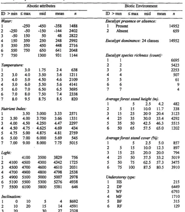
2.2.4 Quantifying ecological variability ... 71
2.2.4. l Regional to local scale environmental heterogeneity ... 71
2.2.4.2 Local scale biotic and abiotic heterogeneity ... 74
2.2.5 Assessing sampling adequacy in eucalypt-forest habitat units ... 75
2.3 Results ... 76
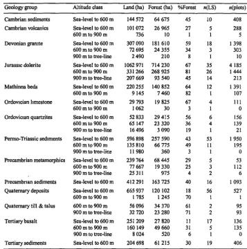
2.3.1 Land systems and eucalypt forest habitat units ... 76
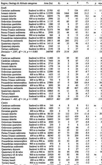
2.3.2 Characterising regional environmental heterogeneity ... 78
2.3.3 Characterising local scale environmental heterogeneity ... 79
2.3.4 Assessing sampling adequacy in eucalypt forest habitat units ... 81
2.3.4.1 Expected sampling frequency: interpolating regional environmental heterogeneity ... 81
2.3.4.2 Expected sampling frequency: extrapolating local environmental heterogeneity ... 87
2.4 Discussion ... 89
2.5 Conclusions ... 93
3. Sampling adequacy of compiled ecological data for representing Eucalyptus species' geographic and environmental ranges ... 96
3. 1 Introduction ... 96
3.2 Methods ... 98
3.2.l Atlas of Tasmanian Eucalyptus species' distributions ... 98
3 .2 .2 Assessing representativeness of Eucalyptus forest community variability ... 99
3.2.3 Assessing sampling adequacy of species' geographic and altitudinal ranges .. 100
3 .2.4 Assessing the samplmg independence of altitude ranges ... 102
3 .2.5 Assessing the complementarity of absence data ... 102
3.2.6 Estimating minimum sampling requirements ... 104
3.3 Results ... 105
3 .3 .2 Assessing sampling adequacy of species' geographic and altitude ranges ... 109
3.3.3 Assessing the sampling independence of altitude ranges ... 119
3 .3 .4 Assessing the complementarity of absence data ... 121
3.3.5 Estimating minimum sampling requirements ... 130
3.4 Discussion ... 137
3.5 Conclusions ... 143
4. Soil water supply: how well does a resource gradient estimated from limited site information predict species' distributions? ... 144
4.1 Introduction ... 144
4.2 Methods ... 148
4.2.l Ecological dataset ... 148
4.2.2 Developing a model of site water balance ... 149
4.2.3 Testing and validating the water balance model ... 152
4.2.4 Water balance variation in Tasmanian eucalypt forests ... 154
4.2.4.1 Modelling performance of individual Eucalyptus species from native forest stands ... 154
4.3 Results ... 155
4.3.1 Testing and validating a water balance model ... 155
4.3.1.1 Western Australian soil moisture data ... 155
4.3.1.2 Eucalyptus globulus plantation sites in Northern Tasmania ... 157
4.3 .1.3 Water balance variation in Tasmanian eucalypt forests ... 162
4.3.2 Modelling performance of individual Eucalyptus species ... 164
4.4 Discussion ... 168
4.5 Conclusions ... 171
5. A case study: mixed-species stands of eucalypts as ecotones on a water supply gradient ... 172
5 .1 Introduction ... 172
5 .2 Method ... 173
5.2.1 Da~base analysis of co-occurrence ... , ... 173
5.2.2 Distribution of mature trees within mixed-species stands ... 175
5.2.3 Stand development ... 176
5.2.4 Species' performance on an artificial soil moisture gradient ... 177
5.3 Results ... 178
5.3. l Database analysis of co-occurrence ... 178
5.3.2 Distribution of mature trees within mixed-species stands ... 180
5.3.3 Stand development ... 181
5.3.4 Physiological responses on an artificial water supply gradient ... 183
5.4 Discussion ... 188
5.5 Conclusions ... 191
6. Productivity gradients: can physiological processes be used as a bioassay of plant responses for predicting species' distributions? ... 193
6.1 Introduction ... 193
6.2 Method ... 195
6.2.1 Ecological dataset ... 195
6.2.3 Eucalypt canopy productivity ... 200
6.2.4 Modelling performance of individual Eucalyptus species from native forest stands ... 203
6.3 Results ... 204
6.3.1 Environmental gradients in temperature ... 204
6.3.2 Eucalypt canopy productivity ... 206
6.3.3 Correlation between environmental variables and productivity indices ... 208
6.3.4 Modelling performance of individual Eucalyptus species ... 209
6.4 Discussion ... 221
7. Modelling the realised niche of Eucalyptus globulus ... 225
7 .1 Introduction ... 225
7.2 Methods ... 230
7 .2.1 Database for occurrences of Eucalyptus globulus ... 230
7 .2.2 Rank order dominance and the calculation ofrelative dominance ... 231
7 .2.2.1 Rank-order dominance ... 232
7.2.2.2 Relative dominance ... 232
7.2.2.3 Calculating relative dominance ... 233
7 .2.3 Patterns of co-occurrence & dominance between E. globulus and other eucalypts ... 234
7.2.3.1 One or two-way patterns of association within the sampling domain for E. globulus ... 235
7.2.3.2 Multiple patterns of association between E. globulus and other eucalypts ... 236
7 .2.4 Biotic explanatory variables ... 23 7 7 .2.4.1 Disturbance processes and structural dynamics of the eucalypt forest ... 23 7 7.2.4.2 Structural attributes of the eucalypt forest stand as an indicator of disturbance cycles ... 238
7.2.4.3 Eucalyptus species richness as an indicator of micro-habitat heterogeneity ... 239
7 .2.4.4 Stand biomass index as an indicator of overall site fertility ... 240
7 .2 .5 A biotic explanatory variables ... 241
7.2.5.1 Climatic water gradients ... 242
7.2.5.2 Climatic temperature gradients ... 243
7 .2.5 .3 Climatic light gradients ... 249
7 .2.5.4 Nutrient indices and E. globulus response ... 250
7.2.5.5 Spatial co-variates ... , ... 251
7 .2.6 Univariate ecological responses ... 253
7 .2. 7 Multivariate ecological responses ... 253
7 .2. 7 .1 Regression modelling methods ... 254
7.2.7.2 Model validation methods ... 256
7.2.7.3 Defining biotic and abiotic attributes for the interpolation grids - data regularisation ... 259
7.2.7.4 Graphic display methods of direct gradient analysis ... 261
7 .2.8 Exploring different aspects of the distribution of E. globulus ... 264
7.2.8.2 Clarifying responses - models of E. globulus dominance and fits with
biotic predictors ... 265
7.2.8.3 Forest type as an indicator of E. globulus ecotypes ... 266
7.2.8.4 Competition with closely related species - E. globulus and the white gum complex ... 267
7.3 Results and discussion ... 268
7 .3 .1 Patterns of co-occurrence & dominance between E. globulus and other eucalypts ... 268
7 .3 .1.1 One or two-way patterns of association within the sampling domain for E. globulus ... 268
7 .3 .1.2 Multiple patterns of association between E. globu/us and other eucalypts 277 7.3.1.3 Hypotheses of association between E. globulus and other eucalypts ... 280
7 .3 .2 Univariate ecological responses of E. g/obulus ... 282
7 .3.2.1 Biotic explanatory variables ... 282
7 .3 .2.2 Abiotic explanatory variables ... 284
7.3.3 Exploring different aspects of the distribution of E. globulus ... 288
7 .3.3.1 Testing the suitability of sample size and representativeness for robust modelling ... 288
7.3.3.2 Modelling the realised niche of E. globu/us in eastern regions ofTasmania ... 294
7.3.3.3 Clarifying responses - comparative performance ofrealised niche models ... 306
7.3.3.4 Forest type as an indicator of E. globulus ecotypes ... 314
7.3.3.5 Competition with closely related species ... 326
7 .4 General Discussion ... 34 7 7.4.1 Methodological considerations ... 347
7.4.1.1 Defining sampling domains ... 347
7.4.1.2 Selecting biotic and abiotic predictors ... 348
7.4.1.3 Defining response shapes by polynomials ... 350
7.4.1.4 Predicting and interpreting probabilities from binary responses ... 350
7.4.1.5 Displaying and interpreting response shapes ... : ... 351
7.4.1.6 Future directions in the development ofrealised niche models ... 351
7.4.2 The realised niche of E. globulus ... 351
7.4.2.1 Ecological responses and physiological processes of E. globulus ... 352
7 .4.2.2 Biotic predictors ... 353
7.4.2.3 Response shapes ...•... 354
7.4.2.4 Ecotypes and competition with the white gums ... 354
8. Linking pattern and process: regression models of plant distribution patterns .... 358
8.1 Introduction ... 358
8.2 Methods and procedures ... 358
8.2.1 What constitutes representative sampling? ... 358
8.2.2 Which environmental gradients are suited to ecological modelling? ... 359
8.2.3 Constrained sampling domains and 'naughty-noughts' ... 361
8.2.4 How should regression analysis be applied to predict species' distributions?. 361 8.2.5 What constitutes a valid prediction? ... 362
8.3.1 Modelling the realised niche of E. globulus ... 362
8.3.2 Interpreting the predictions - direct gradient analysis and distribution mapping ... 3 63 8.3.3 Implications of physiological insight to ecology and land management ... 364
8.4 A systematic approach to correlative modelling of species' distributions ... 365
8.4.1 Future prospects for modelling species' distributions ... 366
8.4.1.1 What improvements are possible in environmental gradient definition? ... 366
8.4.1.2 How can we better define the shapes of species' responses? ... 367
8.4.1.3 How can we improve the modelling methods? ... 367
8.4.1.4 Application of predictive modelling to other biological systems ... 368
8.5 Conclusions ... 368
Figures
Figure 1.1 Generalised system of plant response to an environmental gradient ... 6
Figure 1.2 Plant-stress and plant-productivity functions of an environmental gradient defined relative to the generalised physiological response of a species ... 9
Figure 1.3 The nested arrangement between physiological and ecological responses ... 20
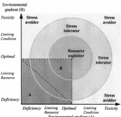
Figure 1.4 Arbitrary classification of plant strategies representing fundamental niche responses .... 29
Figure 1.5 Gradient interpretation of adaptive plant traits from ecological responses ... 29
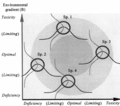
Figure 1.6 Demonstrating a continuum in adaptive plant traits relatJ.ve to two environmental gradients ... 30
Figure 1.7 An imagined distribution ofa species in three landscape categories for an imagined mountain profile ... 34
Figure 2.1 Sampling rules devised by Neldner et al... ... 63
Figure 2.2 Example of observed data spread for 100 randomised resamplings of regional land system heterogeneity in the North-East ... 72
Figure 2.3 Size range of eucalypt forest habitat units in Tasmania ... 77
Figure 2.4 Average replication rate within the sample of observations ... 84
Figure 2.5 The natural log relationship between observed and expected sampling frequency ... 84
Figure 3.1 Range size distributions for the presence of Tasmanian Eucalyptus species in 100 ktn2 cells . . . . .. . ... . . ... . .. . . .. . . . .. . .. . . .. . . ... . . .. . . .. . . .. . . .. . . .. . . 109
Figure 3.2 Tasmanian Eucalyptus species' range-size distribution for log10 transformed geographic range sizes . . . . ... . . .. . . . .. . .. . . .. .. . . .. . . .. . . .. . . 110
Figure 3 .3 Frequency of presence for each Eucalyptus species by taxonomic series in the ecological dataset. . . .. . .. . .. .. . . . .. .. . . ... . . ... .. . . .. . . .. . .. . . .. . .. . .. . . .. . .. . . .. . . 111
Figure 3.4 Distribution records ... 114
Figure 3.5 The relative contribution of altitude information from the ecological dataset. ... 117
Figure 3.6 Comparison of analyses based on presence-only data or presence/absence data ... 123
Figure 3.7a The relative contributions of altitude, latitude and longitude ... 124
Figure 3.7b The relative contributions oflatitude and longitude ... 125
Figure 3.8 Example of climatic envelope for Eucalyptus species' occurrences ... :. 126
Figure 3.9 Box-plots for the univariate distribution of the net water balance variable ... 127
Figure 3.10 Relative substrate fidelity between Eucalyptus pulchella and E. tenuiramis ... 130
Figure 4.1 The continuous relationship between the actual evapotranspiration coefficient and the relative available soil water content ... 151
Figure 4.2 Comparison between observed and predicted soil water contents for Mumbalup and Manjimup ... 156
Figure 4.3 Seasonality and monthly range of actual evapotranspiration, soil water potential and an index of surplus water ... 159
Figure 4.4 Comparison of the degree to which growth of E. globulus at a site is limited by water stress... 160
Figure 4.5 Seasonality and monthly range of soil water potential and soil water runoff for a range of forest habitats ... 163
Figure 4.6 The relationship between two indices for water balance, mean annual soil water potential and total annual soil water runoff ... 163
Figure 5.1 Set diagram indicating the proportion of the data in mixed-species and pure stands .... 174
Figure 5.3. Diagrammatic representation of the transect through a mature mixed-species forest.... 180
Figure 5.4 Predicted abundance of E. obliqua and E. tenuiramis and the
estimated annual mean soil water potential... 181
Figure 5.5 The soil depth and location and height of all trees, and the dominant trees only,
on one of the 400 rn2 lopg-terrn growth plots ... 183
Figure 5.6 Growth and biomass relationships of seedlings from the artificial soil water
supply gradient ... 184
Figure 5. 7 Predawn leaf water potentials of seedlings of both species growing at
different locations on an artificial soil water supply gradient. ... 185
Figure 5.8 Net photosynthesis of E. obliqua and E. tenuiramis growing at different locations on an artificial soil water supply gradient. ... 186
Figure 5.9 Stomata! conductance and instantaneous water use efficiency of E. obliqua and
E. tenuiramis growing at different locations ... 187 Figure 5. I 0 Estimated total canopy carbon fixation per plant of E. obliqua and E. tenuiramis
growing at different locations ... 188
Figure 6.1 Examples of seasonal variation in diurnal temperature defined by an asymmetric
sine interpolation of maximum and minimum monthly mean daily temperatures ... 198
Figure 6.2 Examples of seasonal variation in the diurnal trace of the light-saturated rate of
photosynthesis ... 202
Figure 6.3 Seasonality and monthly range of mean daily temperatures for forest habitats
dominated by Eucalyptus species in Tasmania ... 205
Figure 6.4 Seasonality and monthly range of vapour pressure for a sample of forest habitats
dominated by Eucalyptus species in Tasmania ... 205
Figure 6.5 Seasonality and monthly range of the thermal indices for forest habitats
dominated by Eucalyptus species in Tasmania ... 206
Figure 6.6 Seasonality and monthly range of the average daily rate oflight-saturated
photosynthesis for a standard crop of eucalypts ... 207
Figure 6. 7 Seasonality and monthly range of an indices for canopy productivity in
forest habitats dominated by Eucalyptus species in Tasmania ... 207
Figure 6.8 Examples of the two dimensions of temperature derived from annual and seasonal sets of conditions ... 209
Figure 6.9 Univariate responses to indicative temperature and productivity variables ... 211
Figure 6.10 Bivariate responses to temperature ... 214
Figure 6.11 Gradient comparisons between ecological and physiological responses with
variation in temperature ... 219
Figure 6.12 Outer envelope of predicted ecological responses of four Eucalyptus species
by mean annual carbon gain ... 221
Figure 7. I Putative occurrence of pure and mixed-species stands of two closely related species .. 229
Figure 7 .2 Univariate logistic regression responses for the estimated probability of E. globulus occurrence ... 276
Figure 7 .3 Venn diagram illustrating subgeneric patterns of association between
Monocalyptus and Symphyomyrtus species ... 277 Figure 7.4 Venn diagram illustrating the series patterns of association with E. globulus ... 278
Figure 7.5 Venn diagram illustrating subgeneric patterns of association between E. globulus
and clinal white gum species ... 279
Figure 7.6 A response sequence in stand type between E. globulus or the white gums
in the presence of subgenus Monocalyptus species ... 279
Figure 7. 7 Univariate ecological responses for the estimated probability of E. globulus
Figure 7.8 Selected univariate ecological responses for the estimated probability of
E. globulus occurrence ... 286
Figure 7 .9 Univariate ecological responses for the estimated probability of E. globulus
occurrence ... 287
Figure 7 .10 Discrimination performance of the model for E. globulus occurrence ... 289
Figure 7 .11 Discrimination performance of the model for E. globulus occurrence
relative to abiotic environmental gradients ... 291
Figure 7.12 Discrimination performance of the models for E. globulus occurrence or dominance relative to abiotic or to biotic and abiotic environmental gradients ... 295
Figure 7.13 A direct gradient comparison of the ecological response to annual rainfall ... 301
Figure 7 .14 A direct gradient comparison of the ecological response to minimum
temperature of the coldest month ... 302
Figure 7 .15 A direct gradient comparison of the ecological response to mean annual index of terrain-modified to flat-surface solar radiation ... 303
Figure 7.16 A direct gradient comparison of the ecological response to biotic attributes for
Eucalyptus species' richness and stand biomass index ... 304
Figure 7 .17 Discrimination performance of the models of putative E. globulus ecotypes in mesic and drought-prone habitats relative to abiotic environmental gradients ... 315
Figure 7.18 A direct gradient comparison of the ecological response to annual rainfall and
maximum vapour pressure deficit ... 321
Figure 7 .19 A direct gradient comparison of the ecological response to the index of
terrain-modified to flat-surface solar radiation and nutrient status ... 322
Figure 7.20 Discrimination performance of the models of pure and mixed-stand occurrences of
E. globulus and the white gum complex relative to abiotic environmental gradients .... 327 Figure 7 .21 A direct gradient comparison of the ecological response to the rainfall of the
driest month ... 333
Figure 7.22 A direct gradient comparison of the ecological response to the minimum temperature of the coldest month ... 334
Figure 7.23 A direct gradient comparison of the ecological response to the mean annual index of terrain-modified to flat-surface solar radiation ... 335
Figure 7.24 A direct gradient comparison of the ecological response to substrate nutrient index .... 336
Figure 7.25 A gradient in stand composition between E. globulus and the white gums arrayed along gradients in water and temperature ... 345
Figure 8.1 A flow chart demonstrating a systematic approach to ecological modelling and
Tables
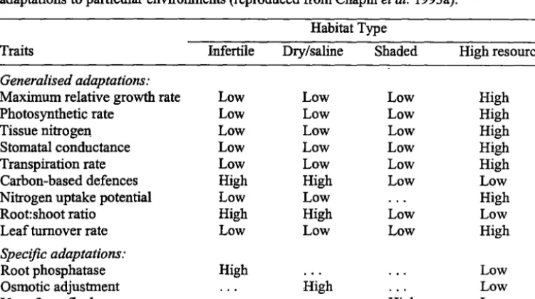
Table 1.1 Generalised suite of traits found in most low- and high-resource environments and specific adaptations to particular environments ... 11
Table 2.1 Ecosystems classification scales and nomenclature ... 62
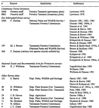
Table 2.2 Sources of collated information, the number of observations in each case, and some associated publications ... 67
Table 2.3 Classification of ecoseries from the biotic and abiotic attributes recorded
in plot samples of eucalypt forest occurrence ... 70
Table 2.4 Spatial stratification rules for undefined levels of spatio-temporal heterogeneity within eucalypt-forest habitat units ... 73
Table 2.5 The number of different environments resulting from a local scale classification of abiotic and biotic attributes ... 75
Table 2.6 Summary ofland systems by regions in Tasmania ... 76
Table 2. 7 Matching between land system and eucalypt forest classifications for areas
representing ecoregions ... 78
Table 2.8 Regional models of environmental heterogeneity defined from the land systems ... 79
Table 2.9 Ecoseries models of biotic and abiotic environmental heterogeneity defined from the biophysical samples in four eucalypt-forest habitat units ... 80
Table 2.10 Relationships between biotic and abiotic environmental heterogeneity in each of four eucalypt-forest habitat units ... 80
Table 2.11 Sampling adequacy of 110 eucalypt forest habitat units across eight regions
in Tasmania ... 82
Table 2.12 Summary of regional sampling adequacy of environmental heterogeneity within eucalypt forest habitat units at the ecosection to ecodistrict scale of ecosystem classific~tion ... 85 Table 2.13 Unrepresented and poorly represented habitat units in the ecological dataset for the
occurrence of eucalypt forest in Tasmania ... 87
Table 2.14 Representation of local scale biotic and abiotic asymptotic heterogeneity within four habitat units ... 88
Table 2.15 Scenarios for the expected number of random samples that would capture
75%, 95% or 99% of the abiotic or biotic heterogeneity ... 88
Table 2.16 Local scale sampling adequacy for representation of75% of asymptotic local scale biotic and abiotic heterogeneity within four habitat units ... 89
Table 3.1 Altitude ranges used in defining species' sampling domains ... 101
Table 3 .2 Representation of eucalypt community variability in the ecological dataset ... 106
Table 3.3 Sampling and replication adequacy for representation of eucalypt community
variability in the ecological dataset... 108
Table 3 .4 Representation of presence and absence, or both response types for each Eucalyptus species in the ecological dataset.. ... 112
Table 3.5 Frequency of presence and absence records, or both response types, for each
Eucalyptus species in the ecological dataset. ... 113 Table 3.6 Relative levels ofrepresentation across each species' known geographic range ... 116
Table 3.7 Representation of altitude ranges for Eucalyptus species in the ecological dataset.. ... 118
Table 3.8 Representation of presences for each Eucalyptus species within 100 m altitude classes for the ecological dataset. ... 119
Table 3.9 Sampling independence of the altitude range for Eucalyptus species ... 120
Table 3.10 Relative contribution of absence information to the altitude response of Eucalyptus species represented in the ecological dataset ... 122
Table 3.12 Biotic environmental heterogeneity of Eucalyptus species' occurrences in the
ecological dataset ... 131
Table 3 .13 Abiotic environmental heterogeneity of Eucalyptus species' occurrences in the ecological dataset ... 132
Table 3.14 Representation in the sampled data domain ... 133
Table 3.15 Representation in the unsampled data domain ... 134
Table 3 .16 Relative representativeness of environmental heterogeneity in the existing sample for each species ... 135
Table 3 .17 Relative habitat differences between Eucalyptus species estimated from the ratio of biotic to abiotic heterogeneity ... 136
Table 4.1 Mean available water retained between -0.01 and-1.5 MPa ... 151
Table 4.2 Average environmental conditions at Mumbalup and Manjimup Eucalyptus globulus plantation sites in Western Australia ... 153
Table 4.3 Range in site information across 19 Eucalyptus globulus plantations in northern Tasmania ... 153
Table 4.4 Annual mean, median and standard errors for the observed and predicted estimates of soil water content over the measurement period ... 15 6 Table 4.5 Evaluating the performance of the water balance model ... 157
Table 4.6 Range in annual site conditions (mean, maximum, minimum) predicted across 19 Eucalyptus globulus plantations in Northern Tasmania ... 158
Table 4. 7 Comparison of estimates of water supply based on the soil water retention function ... 161
Table 4.8 Pearson correlation coefficients between indicative variables from the water balanc~ model ... 162
Table 4.9 Correlations between water balance estimates and climatic variables for a range of forest habitats dominated by Eucalyptus species in Tasmania ... 164
Table 4.10 Univariate ecological responses to water ... 165
Table 4.11 Multivariate ecological responses to water and temp~rature ... 167
Table 4.12 Multivariate ecological responses to water and temperature ... 168
Table 5.1 Tests for significant differences in the soil depth and the annual mean soil water potential associated with dominant individuals ... 182
Table 6.1 Physiological parameters for a standard crop of eucalypts averaged from the published responses of Eucalyptus pauciflora . ... 201
Table 6.2 Pearson correlation coefficients (percentages) for mean annual statistics of the monthly thermal variables for a sample of eucalypt forest habitat in Tasmania ... 208
Table 6.3 Change in deviance (logistic regression) for variables defining thermal conditions of the environment. ... 210
Table 6.4 Bivariate responses to temperature ... 213
Table 6.5 Multivariate responses ... 215
Table 7.1 Biotic and abiotic environmental gradients ... 242
Table 7.2 Seasonal rates of change in environmental temperature ... 247
Table 7 .3 Frequency of presence of each Eucalyptus species in classes ofrelative dominance .... 269
Table 7.4 Paired comparisons for the patterns of E. globulus presence, occurrence or dominance with other Eucalyptus species ... 271
Table 7.5 Spearman rank order correlation coefficients ... 273
Table 7 .6 Patterns of E. globulus presence, occurrence or dominance with respect to a biotic gradient in Eucalyptus species richness ... 284
Table 7.8 The maximum likelihood estimates of the logistic regression parameters for the
realised niche models of E. globulus ... 298
Table 7.9 Fits of realised niche models for E. globulus occurrence or dominance with abiotic
and/or biotic environmental gradients ... 299
Table 7 .10 A direct gradient analysis of the interpolated predictions from the realised
niche models ... 300
Table 7 .11 Spearman rank correlation coefficients between observed probability of
E. globulus occurrence or dominance ... 307
Table 7 .12 Summary of Eucalyptus globulus occurrence by different forest types for the sample
within the geographic and altitude range of E. globulus in eastern regions ... 314
Table 7.13 Maximum likelihood estimates of the logistic regression parameters for models of putative E. globulus ecotypes in mesic and drought-prone habitats ... 319
Table 7 .14 Fits of the logistic regression models for putative E. globulus ecotypes in mesic and
drought-prone habitats ... 320
Table 7 .15 A direct gradient analysis of the interpolated predictions from the models of putative
E. globulus ecotypes in mesic and drought-prone habitats ... 320
Table 7 .16 The maximum likelihood estimates of the logistic regression parameters for the models of pure and mixed-stand occurrences of E. globulus and the white gum complex ... 330
Table 7 .17 Fits of the logistic regression models for pure and mixed-stand occurrences of
E.globulus and the white gum complex ... 331
Table 7 .18 A direct gradient analysis of the interpolated predictions for pure and mixed-stand
Boxes
Box 1.1
Box 2.1
Box 3.1
Box3.2
Box 3.3
Box4.l
Box 6.1
Box 6.2
Box 7.1
Box 7.2
occurrences of E. globulus and the white gum complex ... 332
A systematic approach to the analysis and interpretation of species' distribution·
patterns ... : ... 59
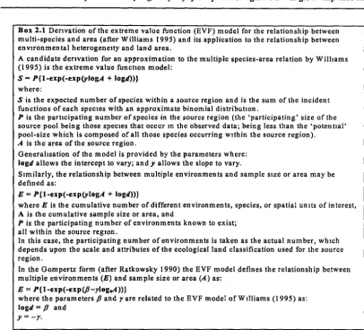
Derivations of the extreme value function (EVF) model for the relationship between multi-species and area ... 73
Empirical calculations developed for the extrapolation of information from the sampled domains of each Eucalyptus species ... 104
Relative suitability of Eucalyptus species for predictive modelling ... 140
Summary of general ecological and taxonomic relations between Eucalyptus species
which may influence exploratory analyses ... 142
Calculation steps in WA TBAL, a simple tipping-bucket water balance model ... 149 Calculation of thermal gradients from the long term estimates for monthly mean daily maximum and minimum temperatures ... 197
Calculating mean daily maximum diurnal vapour pressure deficits from maximum and minimum daily temperatures ... 199
Measuring model calibration and refinement ... 257
Comparing the performance of two or more models where the receiver operator
Maps
Map 7.1 The interpolated distribution of E. globulus occurrence in 100 km2 grid cells in
Tasmania, predicted with average climates in 1 km2 grid-cells ... 293
Map 7 .2A Model A, mean predicted values. The distribution of E. globulus occurrence
predicted with abiotic environmental gradients ... 308
Map 7 .2B Model A, upper 95% confidence intervals. The distribution of E. globulus occurrence predicted with abiotic environmental gradients ... 309
Map 7.2C Model A, lower 95% confidence intervals. The distribution of E. globulus occurrence predicted with a biotic environmental gradients ... 310
Map 7.3 Model B. The interpolated distribution of E. globulus dominance, predicted with
abiotic environmental gradients ... 311
Map 7.4 Model C. The interpolated distribution of E. globulus occurrence predicted with
biotic and abiotic environmental gradients ... 312
Map 7.5 Model D. The interpolated distribution of E. globulus dominance, predicted with
biotic and abiotic environmental gradients ... 313
Map 7.6 Model Wet. The interpolated distribution of E. globulus occurrence in
wet forest stands, predicted with abiotic environmental gradients ... 324
Map 7.7 Model Dry. The interpolated distribution of E. globulus occurrence in dry forest
stands, predicted with abiotic environmental gradients ... 325
Map 7.8 Model A, E. globulus pure stands. The interpolated distribution of E. globulus occurrence in pure stands (in the absence of a white gum species),
predicted with abiotic environmental gradients ... 339
Map 7 .9 Model B, white gum pure stands. The interpolated distribution of white gum species' occurrence in pure stands (in the absence of E. globulus), predicted with abiotic
environmental gradients ... 340
Map 7.10 Model C, Mixed species stands. The interpolated distribution of mixed-species stands comprising both E. globulus and one or more white gum species, predicted with
abiotic environmental gradients ... 341
Map 7 .11 Model D, Mixed species stands dominated by E. globulus. The interpolated distribution of mixed-species stands where E. globulus dominates the white gums, predicted with abiotic environmental gradients ... 342
1.
Predicting plant distribution patterns: a literature review
This chapter reviews links between recent physiological research and ecological theory as a
guide to the development of a systematic approach to the correlative analysis of plant
distributions.
1.1 Introduction
Land managers often exploit site variability as a means of optimising productivity. They may use
models of plant-environment relationships to match species to the sites on which they grow best,
or to predict the effect of changing a particular land management regime. Detailed experimental
work in plant ecology and ecophysiology has provided the theoretical basis for developing robust
and precise models for growing individual species under specific conditions or estimating
probabilities of occurrence. Unfortunately, it is logistically not possible to study intensively all
species in a timely and cost-effective manner. An interim strategy for evaluating plant
performance is therefore needed (e.g. see Norton & Williams 1992; Ehrlich 1996).
With inventories of species' distributions and associated environmental data, predictive models
of plant performance can be developed rapidly using correlative statistical techniques. To be
useful, these models need to be based on sound ecological theory, and be consistent with the
statistical assumptions of the analysis (Austin et al. 1990; Austin & Meyers 1996). Predictive
modelling therefore provides the link between inventory data and questions of land use planning
and management (e.g. Norton & Williams 1992; Prance 1994; Stork 1994), as well as
opportunities to explore hypotheses about the association of plant species and ecosystem
processes (e.g. Austin & Smith 1989; Austin 1991b; Neilson et al. 1992; Austin & Gaywood
1994). The predictions can subsequently be used to guide and focus detailed observational
studies of population dynamics and/or experimental designs (e.g. Carey et al. 1995b).
Some recent developments in ecological theory have implications for the way in which a
correlative analysis of species' distributions may be undertaken (e.g. Austin & Smith 1989).
These developments have arisen largely from physiological research on individual species and
foreshadow new directions for ecological study (e.g. Chapin et al. 1996b; Steffen et al. 1996b).
Previous ecological theory arose from an holistic study of patterns of species' occurrence within
plant coJ:Jllllunities (e.g. Clements 1936; Watt 1947). A more recent reductionist approach, based
on an understanding of physiological and population processes, is increasingly being applied to
the prediction of plant distribution patterns (e.g. Smith & Huston 1989; Bugmann 1996b).
Correlative analyses of species' distributions provide an interim strategy for understanding
Chapter One· Predicting Plant Distribution Patterns
reductionist approach is used to guide the choice of response and explanatory variables in the
model, then there is a greater potential for extrapolating the predictions.
1.2 The biological foundation of vegetation-environment correlation
1.2.1 Vegetation patterns
Vegetation patterns are highly correlated with environment, but different processes dominate at
different scales. For example, Coughenour and Elis (1993) found that ecosystem structure in dry
tropical environments was hierarchically constrained by physical factors: (i) by climate at
regional to continental scales; (ii) by topographic effects on rainfall and landscape water
redistribution, and geomorphic effects on soil and plant available water at the laµdscape to
regional scales; and (iii) by water redistribution and disturbance at local and patch scales. Neilson
et al. (1992) suggested that such vegetation-environment relationships are more than simply
correlations, but are mechanistically founded in the water balance and thermal regimes of a
region.
At continental and global scales, climatic extremes of temperature and moisture are important
determinants of the distribution of major physiognomic types (Woodward 1987). Each
physiognomic type is characterised by a different physiological response, according to its
mechanisms of tolerance and sensitivity to chilling, freezing or desiccation (e.g. Sakai & Weiser
1973). Therefore, each physiognomic type has a competitive edge for a specific combination of
climatic conditions (Woodward 1987; Woodward & Williams 1987).
At regional and local scales, the obvious correlation between assemblages of species and the
environment led to the belief that plant communities are the fundamental unit of organisation in
vegetation (e.g. Clements 1936). However, dynamic and transient associations of individual
species also contribute to plant community diversity (Gleason 1939, Whittaker 1975). The
individual plant response to the environment determines whether it may occupy a particular
micro-habitat (e.g. Menges & Kimmich 1996; Rusch & Fernandez-Palacios 1995). Competition
with neighbouring plants of different species will also influence the presence of individual plants,
and ultimately, therefore, the population density of species (e.g. Burton & Bazzaz 1995; Hara et
al. 1995). Changes in climate or the micro-habitat will lead to further changes in the way species
interact, altering the structure and/or composition of the community (e.g. Aguilera & Lauenroth
1995; Bazzaz et al. 1995). The plant community is therefore a phenomenon of a particular time
and location, at a particular scale of observation. It is therefore a convenient unit for summarising
and communicating complex interactions (Gleason 1939; Austin & Smith 1989).
1.2.2 Species' distributions
Species' distribution patterns reflect the physiological response of individual plants to the
Chapter One: Predicting Plant Distribution Patterns
several generalisations are necessary to successfully predict species' occurrence and apply it to
future scenarios of environmental type (Chapin et al. l 993b ).
Firstly, each species shows a unique response to climate. Therefore, climatic change can cause
species to migrate and/or form new associations (e.g. Nowak et al. 1994; Starfield & Chapin
1996; Watts et al. 1996). However, the individualistic response of species and their interactions
with other species make it difficult to decide which aspects of climate are critical determinants of
distribution. This makes prediction of of future distribution patterns difficult, especially when
relationships are based on the correlation between species' occurrence and environment.
Secondly, changes in the distribution of a species may lag significantly behind climatic changes
where there are limits to the rate of species migration (e.g. Prentice et al. 1991 ). Thus, prediction
of the future response to climate requires some understanding of factors governing the
regeneration phase (e.g. Battaglia 1997; Russell-Smith 1996).
Thirdly, plant response depends on interactions with other species in the community and on
environmental factors other than climate. For example, individual plants are sensitive to the
availability of soil resources and the combination of competitive or facilitative interactions with
other organisms in acquiring limiting nutrients (e.g. Chapin et al. 1986; Turkington et al. 1993;
Turkington 1996). Plant distribution is also related to barriers to dispersal and the distribution of
predators and pathogens (e.g. Loehle & le Blanc 1996), as well as disturbance regimes, such as
fire (e.g. Barton 1993). Therefore, knowledge of climate alone is not enough to project speci~s·
responses into the future or onto different sites. Furthermore, complex and diverse communities,
such as dry or wet tropical forests, have so many key stone species that it is unlikely climate
could be used as the primary mechanism for predicting future vegetation change (Chapin et al.
1993b).
To overcome the inherent difficulties in predicting species' distributions, many workers have
turned to functional groupings of species as a means of reducing the inherent complexity that
needs to be considered when defining scenarios of future response (e.g. Smith et al. 1993;
Steffen 1996; Woodward & Cramer 1996). For example, functional type classifications have
been used to predict vegetation patterns by simulating responses to the environment (e.g. Chapin
et al. 1996a; Steffen et al. 1996a), and for interpreting a functional basis for species' responses
from the correlation of their distribution patterns with environment (e.g. Rutherford et al. 1995).
While simulation studies provide a means of testing the practical and theoretical application of a
functional type classification, the lack of experimental data for individual species, but extensive
floristic inventories, makes the interpretation of species' responses from correlative analyses an
Chapter One: Predicting Plant Distribution Patterns
1.2.3 Operational environment
The prediction of plant species' distributions requires an operational definition of environment
(e.g. Mason & Langenheim 1957; Waring & Major 1964; Emmingham 1978; Mooney & Chapin
1994 ). The environment of a plant is a reflection of a complex history of interactions between
climate, substrate, disturbance, vegetation, fauna and other life forms (e.g. Major 1951). For
practical reasons the description of environmental variation often requires the use of scalars,
indices and surrogates (e.g. Loucks 1962; Austin et al. 1984, 1990; Nemani et al. 1993; Sullivan
& Chesson 1993; Ferrier & Watson 1996; Faith & Walker 1996). The operational definition of
environment and choice of explanatory variables associated with a response therefore depends
upon the scale and purpose of the study.
For the purpose of modelling plant distributions, the choice of sample size depends upon the
environmental space that is utilised by an individual of the target species and the neighbouring
plants that may directly or indirectly influence it (e.g. see discussion by Kenkel et al. 1989;
Tothmeresz 1995). For example, the appropriate scale for sampling the community and
environmental context for a population of mature forest trees might be in the range 0.1 to 0.3 ha.
This reflects the scale of experience of the environment by generations of interacting tree species
at a site. In the case of floristic inventories, the performance of a population at a site may be
simply interpreted as either the presence or absence of the target species. Many such observations
at different sites represent a sample of the species' geographic distribution.
Samples of a species' distribution based on spatial observations of occurrence or relative
performance are relatively simple to collect and large data sets can be efficiently accumulated
from a range of sources (Austin 1991 b ). Despite their obvious value, fewer samples of
within-site monitoring of the cyclical changes of species' response with season or disturbance exist
because of the increased expense involved in establishing permanent plots, and the extra time
required for data collection before analysis (e.g. Fahrig et al. 1994; Herben 1996; Debussche et
al. 1996; Condit et al. 1995, 1996a). Therefore, descriptions of the environment are usually
limited to spatial properties. However, temporal heterogeneity in environment caused by
disturbances, such as fire, flood and landslide are known to influence the developmental stage of
the vegetation (e.g. Barton 1993; Iwasa & Kubo 1995; Barnette & Amoros 1996). As a result,
correlations of species' distributions with their current environment will have residual
unexplained variation.
The biotic habitat associated with a species may be viewed as an emergent property of the
vegetation (sensu Austin & Smith 1989; Austin & Gaywood 1994) reflecting the combined
effects of spatial and temporal heterogeneity in the environment (Stevenson 1997). Factors of
plant community structure and composition reflect these accumulated differences in environment
between sites. For predictive purposes, biological attributes may be suitable surrogates for
unexplained variation in habitat heterogeneity due to temporal effects, when used in combination
Chapter One: Predicting Plant Distribution Patterns
characteristics). In addition, because of the inherent variability in the position of a site within its
cycle of disturbance and succession (e.g. trajectory models by Noble & Slatyer 1980, 1981;
Moore & Noble 1993; Noble & Gitay 1996), replicate samples of similar types of habitat may be
needed when using biological surrogates as explanatory variables in models of plant response.
The interpretation of successional patterns from plant distribution patterns may be possible across
habitats that appear similar except for variation in the developmental stage of the vegetation. This
corollary ofrelating species' distributions observed across many places at one point in time to
indicate trends in successional processes and responses at one place has been a long-held premise
of plant ecologists (e.g. Gleason 1939; Watt 1947; Whittaker 1967). This is much the same as
using the spatially-correlated patterns of species' response to predict scenarios of changing
vegetation and species' distributions with shifts in climate, disturbance or land use (e.g. Huntley
et al. 1995). However, other studies suggest that the interpolation of temporal processes from
spatial observations may not be appropriate, because the properties of species that determine
their long-term spatial dynamics are not the same as those which determine behaviour during
succession (e.g. Prentice et al. 1991; de Swart et al. 1994; Sykes & Prentice 1995, 1996).
In undertaking correlative analyses, the use of attributes for vegetation structure and composition
as surrogates for the influence of temporal processes on the outcome of plant responses does not
necessarily resolve the question of which attributes of climate, substrate or disturbance have been
omitted in a spatial study of plant distribution patterns. However, deduction from a knowledge of
which factors are important to plant distributions and which have already been included in an
analysis may help resolve these issues. The following sections therefore review the physiological
basis of plant response in more detail.
1.3 Physiological responses
The accumulation of physiological responses by many genotypes to their environment gives rise
to species' distribution patterns. The physiological response curve of a plant reflects the diffenng
environmental conditions in which survival, growth and reproduction are possible (Fig. 1.1 ). The
form of the plant response to increasing levels of a factor (termed environmental gradient) is
characterised by an optimum region, either side of which performance (e.g. abundance, growth,
rate of photosynthesis) declines (e.g. Tenhunen & Westrin 1979; Wilson & Keddy 1985; Austin
& Smith 1989; Austin 1992; Sultan & Bazzaz 1993a-c; Sands 1996).
The optimum response of a species to increasing levels of an environmental factor reflects the
range of conditions in which plants grow and reproduce best and leave the most successful
descendants (e.g. Jaindl et al. 1995; Barton & Gleeson 1996; Hansen et al. 1996). However,
plants may also survive over a wider range of conditions than those in which they can grow (e.g.
Dias-Filho & Dawson 1995) or may grow over a wider range of conditions than those in which