heavenly bodies, both fixed stars and planets, with incredible delight; and, when I saw the very great number, I began to consider about a method by which I might be able to measure their distances apart, and at length I found one. And here it is fitting that all who intend to turn their attention to observations of this kind should receive certain cautions. For, in the first place, it is absolutely necessary for them to prepare a most perfect telescope, one which will show very bright objects distinct and free from mistiness, and will magnify them at least 400 times, for then it will show them as if only one-twentieth of their distance off. For unless the instrument be of such power, it will be in vain to attempt to view all the things which have been seen by me in the heavens, or which will be enumerated hereafter.
HIGH-SPEED ASTRONOMICAL PHOTOMETER
by
K. M. Hill, B.Sc. (Hons.) University of Tasmania
A thesis submitted in fulfilment of the requirements for the degree of
Doctor of Philosophy at the
University of Tasmania
This thesis contains no material which has been accepted for the award of any other higher degree or graduate diploma in any tertiary institution, and to the best of my knowledge and belief this thesis contains no material previously published or written by any other person, except where due reference is made in the text of this thesis.
The research programs reported herein have benefited from the contributions, both large and small, of many co-workers, associates and friends.
I would like to express my sincere gratitude to Dr. R.D. Watson and Dr. M.D. Waterworth for their supervision and support. In particular Dr. Watson for his invaluable discussions relating to the observing programs and for his helpful criticisms of the thesis draft.
I also wish to thank Mr. C.M. Ashworth for his helpful discussions relating to electronic matters, the design and building of the counter boards and his help with some of the observations. As with all things mechanical, parts of a telescope system invariably fail or require design modifications to suit particular needs. For this work I would like to thank Mr. D. Phythian for his care and precision in performing such tasks.
I am also indebted to Dr. D.P. Sharma for extra data on EX Hya, brought by him from India, and his keen interest and help with observations in the latter stages of the EX Hya observing program. I must also thank Mr. S.W. Dieters for the help with the 1986 AAT spectroscopic observations, for interrupting his observing program to obtain the 1987 spectroscopic run on EX Hya, and finally for the many nights he assisted with the Mt Canopus observations. For providing a copy of the FIGARO data reduction software, used to process the EX Hya spectra, I would like to thank Dr. K. Shortridge of the AAO.
I thank Dr. A.B. Giles for the inspiration for the AUSSAT observations (Section 5.3), his assistance with the observations, and for the fruitful discussions we had concerning the results of my analysis of the AUSSAT data. More recently, I would like to thank Mr. P.M. Green for his assistance with the SN1987a observations.
I would also like to acknowledge the contribution of Profs. W.B Hubbard and D.M. Hunten, of the Lunar and Planetary Laboratories of the University of Arizona, for their development of a model of Pluto's atmosphere and its application to the Mt Canopus occultation light curve. I also appreciate the predictions of possible occultation events provided by Mr. M. George.
This dissertation describes the development and implimentation of a computer-based photometric data acquisition system for the Mt Canopus telescope. The high-speed photometric system allows continuous acquisition of data, for up to —69 min with a maximum sample rate of 9.8 kHz, while providing a real time display of the counts. The system was thoroughly tested with a pulsing LED source and with observations of the Crab pulsar. The results from several observational programs, suited to the system's capabilities, are also presented. The observational programs involved a study of the DQ Her type cataclysmic variable EX Hydrae, a fast photometric study of geostationary spin-stabilised satellites, a monitoring program on SN1987a, and an occultation program which culminated in a successful observation of a Pluto occultation and the detection of an atmosphere on this planet.
The Mark I version of the fast-photometer system was used for the photoelectric study program on the eclipsing cataclysmic variable EX Hya. This program demonstrated the continued secular decrease in the period of its 67 min modulation. The observed rate of change of the 67 min period implies a mass transfer rate of the order of —3x10-11 Mo yr-1 and a magnetic moment around 8x10 32 G cm3. Two variations in the eclipse timings are also identified. Firstly, one sees a long-term variation that has been fitted with an —20 yr period sinusoid. Secondly, one sees a short-term variation which is correlated with the phase of the 67 min cycle. This second variation has been interpreted in terms of the eclipse of an accretion column or arc in the region above the magnetic pole of the white dwarf.
CONTENTS
Title page
Declaration ii
Acknowledgements iii
Dedication iv
Abstract
Contents vii
Chapter 1: Introduction
1.1 Fast photometry in astronomy 1
1.2 Background to this thesis 2
1.3 Related Technical Work 4
1.4 List of publications 4
Chapter 2: Development of a Fast Photometer system for the MT Canopus 1 m Telescope
2.1 Introduction 6
2.2 Cassegrain design 8
2.3 The cassegrain TV guider/finder system 8 2.4 The photometer optical and mechanical design 11 2.5 Instrument control at cassegrain 13 2.6 The photometer data acquisition system 14
2.6.1 Mark I hardware 15
2.6.2 Mark I software 17
2.6.3 Mark II hardware 21
2.6.4 Mark II software 24
Chapter 3: The Cataclysmic Variables
3.1 Introduction 29
3.2 Observations and classification 30
3.2.1 Classical novae 30
3.2.2 Recurrent novae 31
3.2.3 Dwarf novae 32
3.2.4 Nova—like variables 35
3.3 The binary model 37
3.3.1 Mass transfer 38
3.3.2 The secondary star 40
3.3.3 The accretion disk 41
3.3.4 The hot spot 43
3.3.5 The boundary layer 45
3.3.6 Systems with magnetic primaries 46
3.3.6.1 AM Her systems 46
3.3.7 Outburst models 49 3.3.7.1 Classical and recurrent novae 50
3.3.7.2 Dwarf novae 51
3.4 Conclusion 53
Chapter 4: A Spectroscopic and Photometric Study of the Cataclysmic Variable EX Hydrae
4.1 Introduction 54
4.2 An overview of EX Hydrae 55
4.3 Mt Canopus photometry 56
4.3.1 Observations and data reduction 56 4.3.2 Properties and characteristics of the light curves 58 4.3.3 The orbital period and eclipse timing 70
4.3.4 The 67 minute period 72
4.3.5 Eclipse time residuals and the 67 min modulation 77 4.4 Anglo—Australian telescope spectroscopy 80 4.4.1 Observations and data reduction 80 4.4.2 General spectral characteristics 87
4.4.3 Spectra through eclipse 95
4.5 The accretion curtain model of EX Hydrae 99
4.6 Conclusion 105
Chapter 5 Ultra—high Speed Photometry with the Mark II System
5.1 Introduction 107
5.2 System testing and periodic signal analysis 108 5.3 Observations of geostationary spin—stabilised satellites 116
5.3.1 Observations 116
5.3.2 Period searches and data analysis of
specular reflection episodes 119
5.3.3 Satellite features detected 129
5.3.4 The reflection geometry 130
5.3.5 Satellite eclipse observations 133 5.4 Observations of the Crab pulsar 133 5.5 Ultra—high speed photometry of SN1987a 139
5.5.1 Observations 139
5.5.2 Results and discussion 141
5.6 Observation of a grazing stellar occultation by Pluto 150
5.6.1 Stellar occultations 150
5.6.2 Observations of the P8 event 152
5.6.3 Results and discussion 156
5.7 Conclusion 163
Chapter 6 Conclusions 164
Appendix 1 167
Chapter
1
INTRODUCTION
1.1 Fast Photometry in Astronomy
Astronomical photometry has evolved in step with advances in detector technology from early visual measurements, through photographic measurements, photo-electric measurements with photomultiplier tubes, and most recently to solid state detector measurements using such devices as silicon photodiodes, photodiode arrays, and two dimensional charge-coupled devices. Photographic plates permit integration of light from faint sources and are subject to a more reliable calibration process than are visual measurements. However, they have a limited dynamic range and a non-linear response. Photomultiplier tubes permit only the detection of a single source, but have a larger dynamic range and are linear devices. Also they have much higher quantum efficiencies than do photographic plates. Parallel with the advances in astronomical detector technology have been immense advances in data acquisition and handling techniques, through the development of high-speed digital computers, mass storage devices and data analysis software. They have permitted the full potential of the photomultiplier tube, as a detector in observational astronomy, to be realised. With suitable electronics it has become possible to detect the arrival of individual photons, and hence record the number of photons arriving in a very brief time interval, allowing the study of short-timescale phenomena in optical astronomy
Crab pulsar. Since that time a great variety of stellar phenomena have been examined by fast-photometric techniques, as outlined by Warner (1988). These include the study of stellar occultations by solar system objects, the rapid changes in brightness associated with flare stars, the highly variable light curves of cataclysmic variable stars, the short period and transient features in the light from the X-ray binaries and gamma-ray bursters, some radio pulsars at optical wavelengths, and pulsating stars such as the ZZ Ceti and rapidly varying Ap types.
1.2 Background to this Thesis
The University of Tasmania's lm telescope (the Mt Canopus telescope) is located close to the city of Hobart. The instrument was conceived in the 1970's and became operational in the early 1980's. It is fitted with a dual channel photometer at a folded Cassegrain focus. It has a TV guiding/finding system employing a 15 cm (f/15) finder telescope with a limiting magnitude of mv —12.5 to —13.5, depending on seeing conditions. A guiding/finding system mounted at Cassegrain focus was installed in 1986, thus increasing the limiting magnitude for acquisition and eliminating differential flexure problems between the finder telescope and the main telescope. A complete description of the original telescope system is given by Waterworth (1980). The frontispiece shows a photograph of the Mt Canopus telescope, obtained by taking a time exposure while rotating the dome with the slit open.
The aim of this thesis was to develop a computer-based photometric data acquisition system for the Mt Canopus telescope, in a form which would permit fast photometric observations to be undertaken, and then to use this system to tackle several observational programs which would be permitted by the system capabilities. The observational programs that were selected involved a study of the DQ Her type cataclysmic variable EX Hydrae, a fast photometric study of geostationary spin-stabilised satellites, a monitoring program on SN1987a, and an occultation program which culminated in a successful observation of a Pluto occultation and the detection of an atmosphere on this planet. The thesis work was undertaken on a half-time basis during the period 1982 to 1989.
in the development of this fast—photometry system necessarily fell within the overall financial constraints of a very small annual budget. This was combined with the limited manpower of one person for telescope and observatory maintenance, and another approximately half-time position for technical support. These restrictions have consequently resulted in the slow development of the system.
Following Chapter 2, the next two chapters of the thesis relate to the photometric program on EX Hya, which was supplemented by data from two short spectral runs on the Anglo-Australian telescope. The study of a cataclysmic variable was decided upon as being consistent with the moderate time resolution capability of the Mark I system, a fact which was dictated by limited computer resources. It was also consistent with the limited photometric quality of the observing site, where only 3 to 4 full nights of photometric quality occur per month. My observations during a 1982 pilot program on V1223 Sgr, to help document the period and phase of its then newly discovered 746 s periodicity, had affirmed the suitability of such a cataclysmic variable study. The choice of the particular object for study , EX Hya, was based on the fact that it was a DQ Her type system with a number of interesting, but not fully understood, observational properties. Further it was a relatively bright southern object, of about 13th magnitude. It could therefore be readily studied at the southerly latitude of Mt Canopus, and would also be visible on the original TV guider/finder telescope attached to the 1 m telescope. Chapter 3 of the thesis is intended to present only a brief review, of the observational aspects of, and binary model for, cataclysmic variables, preliminary to the present photometric study. The results of this photometric study are then set out in Chapter 4, and are discussed in relation to an accretion model for EX Hya.
1.3 Related Technical Work
The work presented in the thesis should be considered in the context of the large amount of instrumental development and equipment testing associated with producing the final working system. This more technical aspect of the work was necessary in light of the restrictions imposed by a very small annual budget and minimal manpower. Thus, in addition to developing the photometer system, and the large amount of related software required for such a system, a considerable amount of time and effort was also necessarily spent in the following general areas normally undertaken by technical staff at professional observatories:
—General telescope maintenance. This included removal and installation of the mirrors for re-aluminizing, implementing minor telescope modifications to improve the telescope's performance, and help with the repairs when equipment failed; —Input into the design and testing of the Cassegrain TV guider system discussed in
Chapter 2. This included modifications to the first version of this system, which resulted in an improved ability to focus objects for both the on-axis and offset guiding positions;
—Installation, repair, and maintenance of the computer system and i,ts associated equipment, such as magnetic tape drive, plotters, printers and terminals;
Initial testing and setup of the photomultiplier tubes, HV power supplies and pre-amps. The cold boxes for the PM tubes also required periodic maintenance to check for moisture and to ensure that the front window was clean and the heater element was functioning correctly;
—Help with the initial testing and calibration of shaft encoders, which were installed to improve telescope positioning;
The development of dry-ice making facilities for cooling the PM tubes; —Observational support for other observers.
Hence in addition to the observational results described directly in the thesis, I see my contribution as being important in having provided a new and useful instrument for general research at the observatory.
1.4 List of Publications
material in all of these papers, except the one on V1223 Sgr.
1. "Further Observations of EX Hydrae", K.M. Hill and R.D. Watson: (1984), Proceedings of the Astronomical Society of Australia, 5, 532.
2. "Polarimetry, Photometry and Spectroscopy of the Intermediate Polar V1223 Sgr", D.J. Watts, A.B. Giles, J.G. Greenhill, K.M. Hill, and J. Bailey: (1985), Monthly Notices of the Royal Astronomical Society, 215, 83. 3. "EX Hydrae Timing Data", K.M. Hill, D.P.Sharma and R.D. Watson:
(1986), Proceedings of the International Astronomical Union Symposium No. 118., ed J.B. Heanishaw and P.L. Cottrell, D. Reidel, Dordrecht, 289. 4. "Optical Observations of Geostationary Spin-Stabilised Satellites", A.B.
Giles and K.M. Hill: (1988), Astrophysics and Space Science, 147, 359. 5. "Occultation by Pluto", R.D. Watson, K.M. Hill, S.W. Dieters: (1988),
International Astronomical Union Circular, No. 4612.
6. "Occultation Evidence for an Atmosphere on Pluto", W.B. Hubbard, D.M. Hunten, S.W. Dieters., K.M. Hill and R.D. Watson: (1988), Nature, 336, 452.
7. "Fast Photometry of the Crab, SN1987a and AUSSAT", K.M. Hill, A.B. Giles and R.D. Watson: (1989), Proceedings of the Astronomical Society of Australia, 8, 75.
8. "Supernova 1987a in the Large Magellanic Cloud", S. Dieters, P. Green, K. Hill and R. Watson: (1989), International Astronomical Union Circular, No. 4773.
9. "The Eclipses of EX Hydrae", K.M. Hill and R.D. Watson: (1990), Astrophysics and Space Science, 163, 59.
DEVELOPMENT OF A FAST PHOTOMETER SYSTEM
FOR THE
MT. CANOPUS lm TELESCOPE.
2.1 Introduction
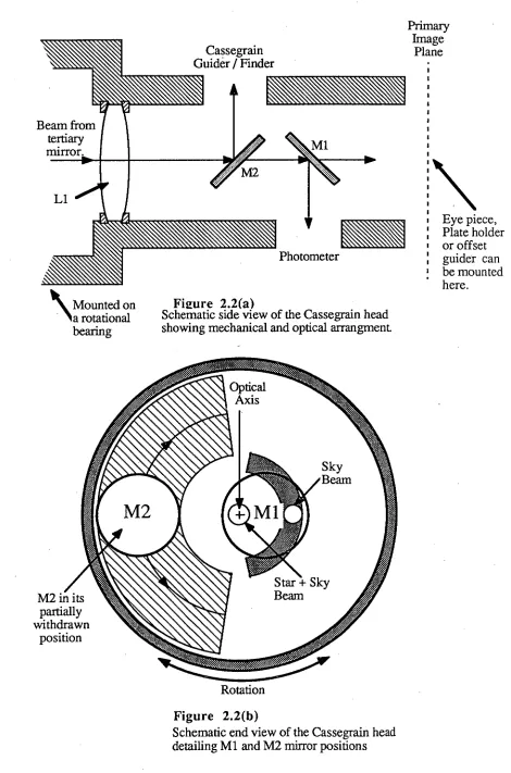
[image:16.557.69.519.82.423.2]The chapter will deal with background details of Cassegrain focus design (Section 2.2), and related details of the Cassegrain TV guider finder (Section 2.3). The design of the Cassegrain photometer is outlined in Section 2.4. Instrument control at Cassegrain is discussed in Section 2.5. The last part of the chapter, Section 2.6, details the hardware and software related to the photometer data collecting system. This was the area of the photometer system design which was implemented by the author while developing a system suitable for fast photometry. Appendix 1 details recent software and hardware developments that allow data to be acquired with a maximum sample rate of 9.8 kHz. Readers wishing only to find out about observational results may omit this chapter entirely and proceed directly to the following chapters.
...r&-we' • ii ( g )
(i)
(i)(h)
( d )
(a) (b) (c)
Guide Scope Image Intensifier Power Supply.
Photometer Cold-Boxes. Photometer Pre-amplifiers. Photometer H.T. Power Supply Cassegrain Instrument
Control Computer. N.D. Filter Drive.
[image:17.556.50.534.51.789.2]Aperture Wheel Controls.
Figure 2.1
Cassegrain TV Guider/Finder. Eye-piece offset Guider.
Cassegrain TV Guider/Finder Mirror Drive.
Guide Scope Image Intensifier and Camera Assembly.
Filter Wheel Drive and Sensor Electronics.
Photometer discriminators and Line Drivers.
2.2 Cassegrain Design
Possible light paths at the f/11.3 Cassegrain focus of the lm telescope are shown in Figures 2.2(a) and 2.2(b) . The main features to note are as follow.
The incoming light beam passes through an aspheric Gascoigne corrector lens (L1), which is used to reduce astigmatism in the primary image. The beam may then be intercepted by the mirror (M2) which is used to deflect a section of the primary image into the Cassegrain TV guider/finder system. This mirror is positioned using computer controlled stepping motors and limit switches. It can be located at any position from the optical axis out to the edge of the primary image plane or retracted altogether. If the on—axis beam is not intercepted by M2 it reaches another mirror (M1). This mirror is placed so as to select the on—axis section of the primary image and deflect it into the photometer. The mirror M1 is mounted on a lever arm so that it can be withdrawn to provide an unobstructed view of the primary image. The arm self—locates such that one side of the mirror is on the optical axis and supplies a beam to the star channel of the photometer and the other side of the mirror provides the beam for the sky channel. Finally, if unobstructed by either M1 or M2, the beam may reach the primary image plane. This section of Cassegrain focus is easily accessible and allows other equipment, such as an eyepiece, offset guider or photographic plate holder, to be attached here. Future equipment such as a low dispersion spectrograph, CCD camera or a third photometer channel for simultaneous comparison star measurements could also be attached at this point.
All of the equipment mounted at Cassegrain focus is fixed on a head which is attached to the telescope by a rotational bearing. This is shown schematically in Figure 2.2(b). The ability to rotate about the optical axis is provided for two reasons. Firstly, if a star happens to be in the sky channel of the photometer, then rotating the head moves the sky channel to another position on the sky. Secondly, if there isn't a star in the field of view of the Cassegrain TV guider/finder system for offset guiding purposes, then by rotating the head it is possible to scan a nearby region of the sky for a suitable guide star.
2.3 The Cassegrain TV Guider/Finder System
V
Li
Cassegrain Guider / Finder
Photometer Beam from
tertiary mirror.
fo.
M1
M2 in its partially withdrawn
position
Primary Image
Plane
Eye piece, Plate holder or offset guider can be mounted here.
\
Mounted on a rotational bearingFi2ure 2.2(a)
Schematic side view of the Cassegrain head showing mechanical and optical arrangment
Rotation
Figure 2.2(b)
[image:19.557.63.533.55.766.2]Low Light Level TV Camera.
Image Transfer Lenses
3 Stage Image Intensifier
Neutral Density Filters
[image:20.557.83.472.65.493.2]Fl F2
Figure 2.3
The Cassegrain TV Guider/Finder design
The operation of the Cassegrain TV guider/finder proceeds in the following way. The
original 15 cm finder telescope is used to locate the object field using bright stars. The
mirror M2 is then placed in its full—in position on the optical axis. In this position the
object field is imaged onto the image intensifier as shown in Figure 2.3 . The TV
image of the object of interest is then placed in the position corresponding to the
photometer aperture on a TV screen. The mirror M2 is partially withdrawn to allow the
light from the object to enter the photometer via mirror Ml. The new partially
withdrawn position of M2 is illustrated in Figure 2.2(b). In moving to this position the
mirror M2 is automatically tilted to image the offset field part of the primary image onto the image intensifier.
Once this has been done an offset guide star is chosen from the field, or, if necessary,
the Cassegrain head is rotated to change the field to search nearby fields for a suitable
guide star. Since the offset field is approximately 4 arc min in diameter there is usually
a suitable guide star available on the TV screen without rotating the head. Two neutral
density filters Fl and F2 are used for guiding on bright objects. Together they provide
either a 10, 100 or 1000 reduction in the light intensity.
The real time display of counts versus time from the photometer is used to define the
edges of the photometer aperture accurately on the TV screen. These aperture edges are
marked on the screen around the guide star. Once the setup procedure is completed for
the object star, and any comparison star needed for variable star photometry, the
observation can be commenced. When dealing with a previously unobserved faint
object and its comparison stars, the whole procedure takes from 30 to 60 minutes to
find and centre them. For bright or known stars the procedure takes 10 to 15 minutes.
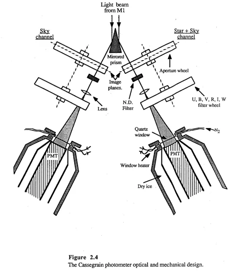
2.4 The Photometer Optical and Mechanical Design
The Cassegrain photometer shown in Figure 2.1 is a dual channel system designed to
make simultaneous 'sky' and 'star+sky' measurements. Figure 2.4 shows the layout
of the system. The photometer design has been described by Waterworth (1980), but a
brief description is included here for completeness.
As shown in Figure 2.4, the light is directed into the photometer using mirror M1 of
Figure 2.2(b). The beam is split with a mirrored prism to form two beams. An on—axis
beam is deflected to the right and an off—axis beam is deflected to the left. Aperture
wheels with six equally spaced holes (6.5, 10, 15, 20, 30, and 40 arc sec. diameter)
Aperture wheel
o/ kfi
Image planes.
N.D. Filter
U, B, V, R, I, W filter wheel
Quartz
window N2
Dry ice Window heater
Light beam from M1
Sky Star + Sky
[image:22.557.63.533.67.626.2]channel channel
Figure 2.4
manually operated from Cassegrain focus. Behind the aperture wheels, neutral density filters are mounted on retractable arms. The sky channel neutral—density filter arm is manually operated from Cassegrain while the star channel one is controlled by computer from the telescope control room.
Lenses (Fabray lens) are used to image the beams onto the photomultiplier tubes by way of filter wheels. Each lens is positioned so that it forms an image of the primary mirror on the photomultiplier tubes. This stationary image helps reduce noise resulting from seeing motion and any sensitivity variations across the surface of the tubes. The filter wheels are similar in construction to the aperture wheels. Five of the six positions available correspond to U, B, V, R and I filters and one is left vacant for white light observations. The filter wheels are operated by computer control from the telescope control room. A heater element surrounds the outer edge of the quartz window on each photomultiplier cold box and a small tube directs dry nitrogen onto the window to prevent fogging.
2.5 Instrument Control at Cassegrain
The Cassegrain photometer and TV guider/finder system have a number of mechanical parts that need to be positioned. In the original system each particular element was manually controlled from Cassegrain focus by the observer. Such a procedure was not satisfactory for two reasons. Firstly, it was time consuming to leave the control room and climb up to Cassegrain focus in semi—darkness, make the changes and return to the control room. Secondly, there are particular telescope positions where it is difficult, or impossible, to reach Cassegrain focus. In these positions it was necessary to move the telescope to make the changes and then move it back to the object.
2.6 The Data Acquisition System
In its original form the Cassegrain photometer data acquisition simply relied on the signals from the photomultipliers being fed directly into counters. These counters were started manually by the observer and remained enabled for a preset period of time. At the end of the preset period, the contents of the counters were displayed on a small thermal printer.
Since then the photometer data acquisition system has undergone two major stages of development. These stages were carried out by the author and other technical staff at the University of Tasmania. The essence of these two developmental stages is as follows:
(i) Mark I System
In the early 1980's, a Digital LSI-11/02 computer and Remex floppy disk drive were added to the system. A counter board was designed and built. The counters plugged directly into the LSI-11 Q—Bus and made it possible for the computer, under program control, to start, stop, read the counters, and store the results on floppy disk.
(ii) Mark II System
In 1987 the data acquisition computer was upgraded to a PDP-11/40, with hard disk drives and a magnetic tape unit. A bus interpreter was used to interface the existing Q-Bus peripherals to the PDP-11 Unibus, and new data acquisition software was implemented.
Both these Mark I and Mark II versions of the data acquisition system have been used to obtain the data presented in this thesis and will be described in more detail in the following subsections. All of the data acquisition software for these versions was written by the author.
2.6.1 Mark I Hardware
Figure 2.5 shows the major components of the Mark I version of the photometric data acquisition system. It was constructed around an LSI-11/02 computer with dual 8" Remex floppy disk drives, which were all available to the observatory.
The photometers are operated in pulse-counting mode. Their output goes directly to low noise pre-amplifiers mounted on the outside of their cold-boxes. The outputs from the pre-amplifiers are taken to noise discriminating, pulse shaping and line driving circuitry. This circuitry consists of low-gain amplifiers with hysteresis set to an optimum level for noise rejection, monostable multi-vibrators to produce a square wave, and line drivers. The pulse width from each monostable multi-vibrator is set at AT=350 ns. Given a true count rate RT counts s-1, the probability of coincident counts is given by -RTxAT. Thus one percent coincidence occurs at -28600 counts s-1. To decrease the effect of coincident counts at high count rates it would be necessary to improve the line driver circuitry. This would allow a smaller value of AT to be used. However, since the count rate in white light from a magnitude 12 star is of the order of 9,500 counts s-1, (depending on the condition of the mirrors), coincidence is not generally a major problem. For bright objects where coincidence is significant, neutral density filters are available. It is also possible, under most circumstances, to correct the data during data analysis.
EMI 9658A
P. M. Tubes Discriminators,
Low Noise Pulse shapers, Pre-Amps. ' and line drivers
( SKY
( STAR
DOME
2 x 50f2 Coaxial Cable. Digital LSI-11/02 (RT-11) Matrox Graphics V.D.U.
(Q-Bus
CONTROL:
"I.
ROOM
' II IIII II
:4
II I I
I
Dual counters ,
144 latches and control logic Parallel line Line printer Accurate frequency standard Sidereal/solar clock and frequency
dividers Clock reset
/Time signal
detector
[image:26.557.88.512.66.721.2]Dual 8" Remex floppy disk drives (2x240 Kbytes) Terminal Radio _-receiver 1==1 • • • • Figure 2.5
term spot measurements that were made to check the short-term stability.
When operating, the acquisition system proceeds in the following way. The computer program enables the counters and timing interrupts. Each sample timing pulse then disables the counters, latches the counters into a parallel set of registers, clears the counters and finally re—enables them. This sequence of events results in a 40 ns dead time, which is negligible. The timing pulse is also used to initiate a computer interrupt sequence to read the registers. The whole process continues until the computer program disables the counters and timing interrupts. The absolute start time is obtained by initially reading the solar clock each time there is an interrupt from the counters and delaying data collection until the seconds ticks over. At that point the start time is recorded and data collection is initiated. No other absolute timing information is stored along with the data. The computer stores the counts from both channels of the photometer on the 8 inch floppy disk drive, and uses a Matrox 512x256 pixel graphics board to produce a real time display of the incoming data.
2.6.2 Mark I Software
Two main functions are performed by the data acquisition software. Firstly, it stores the data from the counters, along with other observational information, on floppy disks. Secondly, it provides the observer with a real time display of the incoming data. The real time display of data is used to help define the position of the aperture on the TV guider screen and to monitor the incoming data stream. This monitoring facility provides a sensitive method of detecting guide errors, and cloud and dome obscuration problems.
the two versions of the Mark I programs operate identically. This major storage limitation imposed by the floppy disks was overcome in the Mark II version of the data acquisition system. The Mark II version is necessary if one wishes to acquire useful continuous data streams with sample times of less than 20 ms.
When controlling data acquisition with the Mark I software, commands of the form <esc>n are entered at the computer keyboard. Here n is a number between 1 and 9. The commands initiate the following actions:
(i) <esc>1
To close any existing output file and open a new output file. In doing this the operator is prompted for the following file—header information:
a) A data identification comment. b) The aperture size to be used.
c) The filter to be used (U,B,V,R,I or none). d) The sampling interrupt period to be used. e) An interrupt summing factor to be used.
This information is written to the output file along with the current computer date. The program uses the interrupt summing factor to integrate the data from several samples before writing it to the output file. This facility is useful when a.
particular interrupt sample time is not available. For example, since a 0.5 s interrupt sample time is not available, one would use an interrupt sample time of 0.1 s and a summing factor of 5 to give 0.5 s integrations.
Separate from the file header information, the program also requests a display summing factor to provide a quite distinct integration time for the real time display of data. For example, if data were being accumulated for 0.5 s intervals as above, then it would be possible to have a real time display resolution of 2.0 s by choosing a display summing factor of 20.
(ii) <esc>2
(iii) <esc>3
To disable data acquisition, ending the current run. (iv) <esc>4
To enable the real time display of incoming data. (v) <esc>5
To clear and reinitialise the graphics display. This option is necessary when moving from one source to another. With a display resolution of 1 s, the display buffer would take 512 s to re—cycle. Using this option clears the display buffer immediately.
(vi) <esc>6
To disable the counters and interrupts, write any buffered data to the output file, close the output file and return to the RT-11 operating system.
(vii) <esc>7
To disable real time graphics display. This option disables the display software, thus allowing smaller sample times to be used than those available with the real time display enabled.
(viii) <esc>8
To delete the last data run from the output file. (ix) <esc>9
To swap the real time display between channels. The options available are the star channel, the sky channel, and the difference between them. These options are presented cyclically.
File header Run header Data Run delimiter record Data identification
comment (24 C*1)
Aperture Size Filter Interrupt period (I*2) (C*1) (R*4) Interrupt summing
factor (I*2)
Month,day,year (3I*2) -2 -2 -2 -2
Run BD comment (8C*1)
Unused
(reserved for future use)
Hours, minutes, seconds (3I*2)
Ch A , Ch B
II II
„
(2I*4)
-2 -2 -2 -2
II II tt II II It II It
-1 - 1 - 1 - 1
More Runs
EOF delimiter Run delimiter 7 record
RUN 1-3 4 5 6 8 9-11 13-N N+1
12 I Start time Record
Number
I * 2 = 2 byte integer I * 4 = 4 byte integer C* 1= 1 byte ascii
R * 4= 4 byte floating point
Figure 2.6
time from the run header part of the file, it is then a simple operation to extract a particular section of the run. This second technique was found to be more useful when obtaining long sections of data on a single object inter—dispersed with infrequent, short, comparison star and sky background measurements. The file is written using the Fortran WRITE command and hence buffering of the data is left to Fortran I/0 system. The data are written in a binary format, this method being more efficient in terms of both space and time.
The data acquisition program is divided into two main parts. The first part consists of a controlling program. This part handles operator requests, the real time display of data, and the writing of data to floppy disk. This section of the program is written in Fortran and its structure is outlined in Figure 2.7. The second part consists of the interrupt initialisation and handling routines. These routines are written in the PDP-11 assembly language Macro-11. The structure of the routines in this part of the program is shown in Figure 2.8
The two parts of the program communicate by way of a common section of memory. This consisting of a large ring buffer, an input pointer which is incremented by the interrupt handling routines as new data arrive, an output pointer which is updated by the control program after it has displayed the data and written it to the disk file, and a buffer overflow error flag which is set by the interrupt processing routines and monitored by the control program. It should be noted that the real time display is never updated while there is unprocessed data in the ring buffer. That is, new data are written to the output file and is only buffered for display until the ring buffer is found to be empty. Only at that point is the real time display updated. This method effectively gives data collection a higher priority than data display. The later requires a few tenths of a second to rescale and update the whole screen.
2.6.3 Mark II Hardware
flag set from ew
data?
(i.e. inptr
utptr
Get data from ring buffer and accumulate
them. Any
keyboard commands
Update Ra Display
Print error
message nough
points accumulated
Write results to disk.
Update Display buffer
Move outptr to next ring buffer position.
One of the 9 command options
Figure 2.7
Read solar time (start time) Set ready flag Firsti Read solar time Set interrupt vector to Photon Set interrupt vector to Enable counters and interrupts Read initial solar time. Clear ready flay Return from
subroutine Disable counters and interrupts
Phoint
Move new data into ring buffer
at inptr
Update inptr to next ring buffer posn.
Call 14 and set buffer overflow error flag 23 Photof Return from subroutine Figure 2.8
The interrupt handling routines associated with the Mark I data acquisition
Device PDP-11 Processo
Device A
C14
(Cable) Bus Interpreter
24
Device A'
Device B'
Figure 2.9
The computer configuration used for the Mark H system
The reason for the hardware upgrade was twofold. Firstly, to do high speed photometry of supernova SN1987a a time resolution of less than 1 ms was desirable, and there was a need a need for more disk storage than was currently available on the LSI-11. Secondly, a power supply failure in the LSI-11 caused considerable damage to that computer, necessitating its repair.
Two options were therefore available to us. Either we could repair the LSI-11 and purchase a hard disk drive and controller, or we could use the other observatory computer, a PDP-11/40, previously used for data reduction, and interface the Q—bus peripherals to its Unibus with a bus interpreter. Fortunately an unused bus interpreter existed in the department at the time and was freely available to us. We therefore adopted the second option, because it required little expense, was quick to implement, and provided us with a faster computer which had a magnetic tape drive and hard disk drives attached. At the time of writing this thesis the solar clock has not yet been interfaced to the PDP-11/40; however, this should be accomplished in the near future.
2.6.4 Mark II Software
proposal was to implement a regular monitoring program for SN1987a, to search for evidence of a rapidly spinning neutron star. Since the spin period might be as small as 1 ms the software would be required to sample at a rate greater than 1 kHz. It was assumed that, at least initially, any modulation would be very weak and it would be necessary to collect as much continuous data as possible.
As already mentioned in Section 2.6.2, for high speed photometry the full 32 bit precision of the counters is unnecessary. Thus, as in the Mark I software, two data acquisition programs have been written. The first program is for two channel (16 bit) photometry. This program has been tested with sample rates up to 2.5 kHz. The second program is used for single channel (8 bit) photometry and will work with sample rates up to 7.5 kHz. For illustration, Table 2.1 shows the time taken to collect 20 Mbytes of data, filling a hard disk, for some sample rates, versus the number of channels and the number of bits per channel.
The Mark II software is capable of much higher data rates than the Mark I versions. There are two reasons for this. Firstly, the data are buffered much more efficiently for the disk and are written asynchronously under DMA control. This improved buffering is achieved by accumulating several disk blocks of data within the program, instead of leaving the buffering to the Fortran I/O system, which is not very efficient. System routines are used for initiating the asynchronous write and detecting its completion. Secondly, the real time display software has been improved. All scaling information is entered into the program by the observer as constants before data acquisition is commenced. In the Mark I software they had been calculated from the incoming data and updated in real time.
Table 2.1
The time in minutes to acquire 20 Mbytes of data for various sample rates as a function of number of channels and number of bits per channel.
2 channels
x 32 bits 2 channels x 16 bits 1 channel x 8 bits
Sample 1.0 43.7 87.3 349.5
rate 2.5 17.5 35.0 139.8
The single channel version of the program is a modified version of the dual channel program. The single channel version handles higher sample rates simply because it has only one quarter as many bytes of data to manipulate. Also the code for buffering the data has been improved slightly over the two channel version. It is envisaged that the two channel version will be eventually updated with the same upgraded buffering. This buffering has been optimised by using a single buffer for both input and output. The input routine places new data in a 16K byte ring buffer, and instead of having a separate output buffer, the output routine divides the ring buffer into eight 2K byte blocks. When a block fills up it is written to the output file under DMA control. After the write has been completed, the output pointer is then updated to the next 2K byte block boundary.
As in the Mark I case, the software can be again divided into two parts, consisting of the controlling program and the interrupt processing routines. The interrupt processing routines are virtually identical to the Mark I routines. The only difference is that the section of code dealing with the solar time has been removed. It will be re—inserted when the solar clock is interfaced to the PDP-11/40. The structure of the controlling program is shown in Figure 2.10. This program provides the observer with five options which are initiated by entering the appropriate character on the console keyboard. These options are:
B This causes the program to prompt for the number of samples that are to be accumulated per pixel for the real time (RT) display.
D This option allows the observer to set the displays vertical gain/reduction factor.
G This option causes the program to enable the counters and displays the incoming data on the RT display. It does not save the data on disk. (iv) S This option is used as a switch to start/stop saving data to the disk. It
can only be used while the program is displaying incoming data (i.e. after the G option).
(v) P This option disables the counters and closes the output file if data have
been saved to it.
Figure 2.10
The Mark II control program structure.
I
Updatr,buffer pointers
Add new point to display buffer Set save flag and reset' buffer pointers Update disk buffer pointer in ring buffer
Wait for previous Xfer to complete then initiate DMA write. Disable counters and interrupts Print command error message Disable counters, interrupts and close output file Finish accumulating data for pixel Scale point and update Real Time display
/ Get keyboard
/
commands Get number of points to be accumulated per pixel "BINS" Get the Gain! Reduction factor. Reset all buffer pointers and, enable counters and sampling interrupts Open output filedetermined by two parameters that are chosen before data collection is started. The first of these parameters, BINS, is the number of samples that are to be accumulated per pixel for the display. The second parameter, GR, is a display gain or reduction factor. A positive value of GR is interpreted as a reduction factor and a negative value as a gain. For example, GR = 2 reduces the scale by a factor of 2 and GR = -2 increases the scale by a factor of 2. This method has been used as an alternative to using a decimal value, which would be 0.5 and 2 for the above example, since the software avoids floating-point arithmetic where possible to increase program speed.
Chapter
3
THE CATACLYSMIC VARIABLES.
3.1 Introduction
This chapter is intended as a breif review of the cataclysmic variable (CV) stars, preliminary to the photometric and spectroscopic observations that are discussed in Chapter 4. The reader who is already familiar with the properties of these stars may wish to proceed directly to Chapter 4.
nature of these stars are discussed in Section 3.3.7.
3.2 Observations and Classification
3.2.1 Classical Novae
The classical novae (CN), by definition, have had only one observed outburst. The rise to maximum light is very rapid while the decline is much slower. The pre-novae stars are found from photographic plates to be blue objects that may show slight irregular changes in brightness. The spectra of the novae at minimum light are characterised by emission lines of H I, He I, He II, Ca II and the X4650 CIII/NUI blend. These are superimposed on a blue continuum. A catalogue of light curves of novae prior to outburst is given by Robinson(1975).
The eruptions of CN range in brightness from 7 to 20 mag. (mean -12 mag.) in the optical. They then fade by a similar amount, and are observed to cause shells of material to be ejected with velocities between 100 km s-1 for slow novae and 4000 km s-1 for fast novae. Mass estimates of the ejected material lie in the range 10-4 to 10-5
Mo. The optical rise to maximum is of the order of only a few days. The rise is generally very steep, being 7 to 10 mag in the first 24 hours, followed by a slow rise in the last 1 or 2 magnitudes before maximum. At the slow-down point some novae may stop, or even show a decline, before continuing on to maximum. The total energy output from an eruption is <1045 erg.
The decline rate defines the sub-class of the nova. The fast ones take 10 to 20 days to decline 2 mag from maximum, while the slow ones take the order of 100 days. The fast novae have brighter absolute magnitudes at maximum than slow novae, but may radiate less total energy. X-ray observations of CN in quiescence have shown that the fast novae seem to be more luminous than the slow ones (Becker and Marshall 1981). If this is the case, it enables the speed class of a nova to be determined well after it has erupted.
die away. In both cases, the transition to a slow decline occurs at —6 mag below maximum. The star then gradually approaches the quasi—stable post—nova state, which approximately corresponds to the pre—nova brightness, and often shows rapid low amplitude changes in brightness. The return to pre—nova brightness usually takes the order of a decade or two. Payne—Gaposchldn (1957) in her now famous book, "The Galactic Novae", presents an enormous amount of observational data (including light curves) for these objects.
The optical variability of CN, however, does not tell the whole story. Ultra—violet (UV) and infrared (IR) observations have shown that, while the visible light declines during the first weeks after the eruption, the UV luminosity rises in such a way that the combined optical plus UV power is approximately constant. The IR characteristics are quite different again, with the fast novae showing little or no black—body IR excess. However the slow novae begin to show an IR excess at about the time the UV luminosity commences to decrease. This excess continues to increase for —200 to 300 days after the optical maximum, reaching 5x10⁴ Le in the case of FU Ser (Geisel et al ,1970). Geisel et al attribute the IR excess to heating of dust grains formed in the ejected material. Two possible mechanisms have been suggested for this heating. It may be collisional warming of the ejected material by interstellar gas. Alternatively, it may be the redistribution of the UV into the IR. Observations made by Gallagher and Holm (1974) have discounted the latter possibility because it predicts a remnant temperature of —200 000 °K. This was not supported by UV observations they made of FU Ser with the 0A0-2 satellite. After reaching maximum, the ER decays with a time constant of the order of 100 — 150 days. Thus the total luminosity of the nova may remain high for much longer than is indicated by its optical—band characteristics. Gallagher and Starrfield (1978) and Starrfield and Sparks (1987) have presented excellent reviews of the CN systems.
3.2.2 Recurrent Novae
great as 4:1 . It is, however, quite possible that outbursts have occurred and been missed.
There is strong spectral evidence to suggest that many RN have a giant star for their secondaries. If this is the case, then at minimum light most of their luminosity could be attributed to the giant star. Hence their outburst amplitudes would be similar to those of the CN, for which absolute magnitudes at minimum are much fainter.
3.2.3 Dwarf Novae
Dwarf novae (DN) form the largest of the four sub—classes of CV's, with over 300 known members. They have a rapid nova—like rise to maximum light, but their increase in brightness is only 2 to 6 mag, and they fade back to pre—outburst brightness within 2 to 10 days. The energy liberated during an outburst is typically 1038 to 1039 ergs, compared with —1045 ergs for the CN and RN. The outbursts are repeated quasi—periodically for any particular star. The intervals between outburst range from as little as 10 days to as much as 600 days. Most lie in the range 20 to 50 days. For any particular star the outburst interval varies, but is usually sufficiently constant for a characteristic time—scale to be associated with each star. Unlike the CN and RN, the DN do not show an IR excess on the decline from maximum and there is no evidence for an ejected shell of matter. However, P—Cygni line profiles in the UV are evidence that there is a wind of material moving away from the system during some outbursts. Spectroscopically the DN differ from the CN and RN in that the latter have higher excitation lines and generally their emission lines are stronger. In particular, the A,4650 blend is present and stronger He II emission is seen. At minimum light the CN and RN tend to be brighter than the DN. The CN and RN have mean absolute magnitudes around Mv.---1-4.5 while the DN have My---+7.5. The DN have been grouped into sub—classes U Gem, SS Cyg, Z Cam, and SU UMa according to their outburst characteristics, which are shown in Figure 3.1 and which may be detailed as follows:
(i) The U Gem stars are characterised by two distinct forms of outburst which
depend on the time spent at maximum. These long and short outbursts and are collectively referred to as normal outbursts. The long and short eruptions have a tendency to alternate. The more energetic eruptions tend to be followed by longer intervals of quiescence.
The SS Cyg stars have, in addition to the normal eruptions, another type of
maximum light. They are referred to in the literature as anomalous eruptions. The Z Cam stars are similar to the U Gem stars in that they have normal eruptions. However, their distinguishing feature is that they can stay at an almost constant brightness for extended periods. These standstills almost always occur during the decline from an outburst and at the same point in the decline. They usually last only a few days, but have been known to last as long as several years on rare occasions. The mean energy output during standstill is approximately equal to the mean non—standstill energy output. Typically their outburst period is shorter than average for dwarf novae, being normally less than 50 days.
(iv) The SU UMa sub—class, recently defined by Vogt (1980), are also very similar
to the U Gem sub—class in that they possess the normal type of eruption as well. However, periodically they undergo an extended outburst, called a supermaximum. The supermaxima are 1 to 2 mag brighter than the normal eruptions and generally last longer than the normal outbursts. The super—outbursts have a tendency to be more predictable than the normal outbursts and occur at a rate of one super—outburst per 3 to 10 normal outbursts. The stars that belong to this group also belong to the ultra—short period group, all having orbital periods of less than two hours. DN with outburst periods less than —30 days fall into either this sub—class or the Z Cam sub—class. The two groups are mutually exclusive, with no SU UMa DN having standstills and no Z Cam stars having supermaxima. Glasby (1970) presents a comprehensive list of schematic DN outburst light curves.
The spectra of dwarf novae in their quiescent state are characterised by broad emission lines on a flat or blue optical continuum. The Balmer lines, He I, as well as He II and Ca II to a lesser degree, are present in the optical region. He H tends to be stronger in the CN and RN. The line width can be attributed to Doppler broadening. The Balmer lines and He I lines are double in systems that are highly inclined. Some DN show the absorption spectrum of G and K main sequence stars. However the secondary is not detected in those with an orbital period less than 6 hours. During a DN eruption the continuum becomes brighter and the lines become relatively fainter. At maximum the emission lines are generally replaced by absorption lines, sometimes with weak central emission on the decline from maximum.
, U
I I Gem
,
I I I I I
SS Cyg
I I I I Z Cam
I I I I
I
I
I I I SU UMa
I I I
Time
Figure 3.1
Schematic light curves for four sub—classes of dwarf nova. These light curves illustrate the different types of outbursts.
and 0.1. This can contribute up to 50 percent of the light from a system. One of the better known examples of this is the star U Gem itself. Typically flickering shows up as low amplitude (<1 mag) changes in brightness on a time scale that ranges from seconds to tens of minutes. Photometric studies have shown that the amplitude of the flickering is larger in the UV than at longer wavelengths. In systems with a hump, the flickering is generally larger during the hump and is seen to disappear entirely during an eclipse. Some systems, however, show flickering at all binary phases. Power spectra of the light curves reveal a continuous rise in power towards the lower frequencies, with power tending to rise linearly with f-1. Multi—colour observations of eclipsing systems show that the eclipse width is generally longest in the IR and shortest in the UV.
some DN show low amplitude quasi—periodic oscillations. These usually vary in period, sometimes with a steady drift. At other times the drift is more irregular and with perhaps many periods present at once. Their coherence varies from a few cycles to several hundred cycles. The more coherent cases tend to show an increase in period as the outburst declines. Oscillations are not observed in all DN and on occasions they have failed to be detected in DN that have shown them during previous eruptions. Typically the periods are in the range 10 to 40 s and the amplitudes range from 0.0009 to 0.01 magnitudes.
The hump that is seen at quiescence is only marginally affected by the outburst and its contribution to the total light from the system remains about the same during an outburst. This is evident in U Gem, where the eclipse of the hump—producing feature becomes very shallow during outburst. However, during supermaximum in the SU UMa type stars, the normal hump disappears on the rise to maximum and is gradually replaced with a similar feature that is much brighter than the normal hump (-40 times normal for VW Hydri). This superhump has a period that is 2 to 5 percent larger than the binary period and is even seen in systems with low inclination. On the decline from outburst the amplitude of the super—hump decays more rapidly than the brightness of the star, and eventually the normal hump returns.
Observations of DN with the Einstein X—ray observatory showed them to be low luminosity X—ray sources. In their quiescent state, the ratio of hard X—ray flux to visible flux is approximately unity. However, during outburst the ratio changes so that Lx/Lv 0.06 , indicating that the hard X—ray flux has changed little when compared with the change at optical and UV wavelengths. The soft X—ray luminosity (0.1-0.5 keV), on the other hand, is seen to increase by a factor of —100 for some DN at maximum. This component has an effective black body temperature of kT,-50 eV, implying that much of the emission during outburst is in the extreme ultra—violet (EUV) region of the spectrum. The flickering in simultaneous X—ray and optical light curves correlates well, suggesting that they may be related. In eclipsing systems the hard X—ray eclipse is seen to correspond with the optical one.
3.2.4 Nova—like variables
Nova—like variables (NL), unlike stars in the preceding groups, have not been
do not vary as dramatically as the other classes of CV, and are more difficult to recognise. It is not surprising then, that a relatively high proportion of the NL stars are eclipsing systems, since eclipsing systems are much more noticeable. I will also include three other types of CV under the heading of NL objects. Besides the UX UMa stars (that is classical NL variables), there are the magnetic variables, and the VY Sc! stars. The magnetic variables encompass the AM Her stars, or Polars, and the DQ Her stars, or the Intermediate Polars. The properties of these sub—classes are as follows:
(i) The UX UMa stars resemble DN near outburst or standstill. Typically they show weak He II and X4650 emission or absorption. They can have an orbital hump characteristic of the other CV classes, although it is smaller than those in DN with similar inclination. Their flickering characteristics are similar to the DN. Stars belonging to this class have orbital periods greater than 3 hours.
The AM Her stars are recognised primarily by variations, at the orbital period, in
their circular and linear polarised light. The fraction of polarisation ranges between 10 and 35 percent and is usually strongest at red and IR wavelengths with the exception Of systems with higher than usual magnetic fields (Section 3.3.6.1). These systems don't have eruptions as such, but have on and off states that may last from weeks to years. The on and off states differ in brightness by 3 to 5 magnitudes. The AM Her objects are the strongest X—ray emitters of all the CV's, with Lx/Lv.--10. They show broad Balmer, He I, He II and X4650 single peaked emission lines. When in their off state some of these stars show Zeeman splitting of the emission lines, implying magnetic fields of the order of a few times 107 G. In contrast to the DN, the AM Her stars show strong flickering in the red. This tends to be present throughout the whole orbital cycle. The X—ray spectrum of these stars is composed of two parts, a soft X—ray blackbody component and a hard X—ray bremsstrahlung component. Unlike other CV's the soft X—ray flux dominates their X—ray spectrum.
The DQ Her stars have as their defining characteristic, stable, short period,
coherent variations in their optical and/or X—ray flux. The period of these oscillations ranges from 33 seconds in the case of AE Aqr to 67 minutes for EX Hya. In some systems three separate periods are seen: a longer period associated with the binary orbit, Po; a short period variation in the X—ray and/or optical, P 1; and another short period modulation in the optical, P 2. The periods are related by:
1 1 1
Warner (1982) shows that this relationship is expected if the X-ray/optical periodicity (P1) is due to the rotation of the primary ( see Section 3.3.6.2.). This seems quite likely given the stability of these oscillations ( p/P = -2.7x10⁶ yr-1 for DQ Her itself). Some of these systems have circularly polarised light in the optical, modulated at period P1, (-0.6 percent for both DQ Her and AE Aqr). The polarisation is much weaker than that observed in AM Her systems. This indicates that the DQ Her systems have weaker magnetic fields than the AM Her types. It is believed that the primaries in the DQ Her systems possesses fields of <10 7 G. Finally, it is worth while noting that many DQ Her stars belong to other CV classes. For example, DQ Her itself is also classed as an ex-nova, EX Hya has dwarf nova outbursts and many are classed as nova-like. Similarly several CN exhibit DN outbursts (e.g. Q Cyg, GK Per). This would tend to support the argument that, for CV's in general, we are looking at similar systems, perhaps at different points in their evolution or with only subtle physical differences.
(iv) The VY Scl stars show high and low states. They stay in their high state most of the time and occasionally dim to a low state, similar to the AM Her stars. However, unlike the AM Her objects, their light is not polarised. In their high state they resemble the UX UMa stars. When they dim, they are more like the DN at quiescence. The low states can last from a few weeks up to many months and are 3 to 5 mag fainter than normal brightness. In their low state, their energy distribution is consistent with that of a hot white dwarf. VY Scl stars are sometimes referred to as anti-dwarf novae because, unlike the DN, they spend most of their time in the high state.
3.3 The Binary Model
The standard model for CV's envisages a binary system in which the primary star is a white dwarf and its companion is a near main sequence G, K, or M star, or in some cases a giant star. I will not include in this discussion the AM CVn stars, which have white dwarf secondaries, as they are fundamentally different. Since the majority of CV's are observed to have short orbital periods ranging from -82 min to -16.5 hours (excluding GK Per and T CrB), then by Kepler's third law the distance, a, between the components must be small. We may write this law as
a = 3.5x10 10 x P2/3 x (M1+M2) 113 cm, 3.2
stars in solar masses. If, for example, a system has a total mass of 1Mo and an orbital period of 100 min, then the components will be separated by -4.9x10 5 km, approximately the Earth-Moon separation.
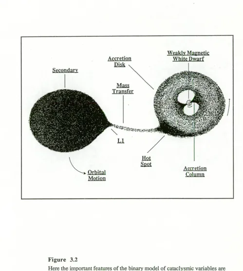
If the secondary fills its Roche lobe, then material will stream away from it through the inner Lagrangian point (L1). The material lost through Li will contain orbital angular momentum and, in the absence of a strong primary magnetic field, will form a disk within the Roche lobe of the primary. Viscosity in the disk will eventually cause the material to be accreted onto the white dwarf surface. The infalling stream from Li forms a hot spot at the impact point with the disk, which manifests itself as the prominent hump seen in the light curves of many CV's prior to eclipse.
If the the magnetic field of the white dwarf is strong enough, then an accretion disk will not form. Instead, the magnetic field will control the flow of matter leaving Li and form an accretion column. This funnels the material onto the surface of the white dwarf near a magnetic pole. The kinetic energy of the infalling material will be released in a standing shock region above the magnetic pole of the primary. It is also possible for intermediate cases to exist, where the magnetic field of the primary is not strong enough to stop the formation of a disk. However, it is strong enough in the inner parts of the disk to disrupt it and form accretion columns onto the poles of the white dwarf. The important features of the binary model are illustrated in Figure 3.2. We will now look at the main theoretical aspects of these systems: mass transfer, the secondary, the disk, the hot spot, the boundary layer between the disk and the white dwarf, the effect of a magnetic primary and outbursts.
3.3.1 Mass Transfer
Accretion Disk Secondary
Weakly Magnetic White Dwarf
il.9.1
Spot Orbital
Motion
Accretion Column
Mass
Transfer
[image:49.556.33.532.52.609.2]Ll
Figure 3.2
mass to spill through Ll. The first of these mechanisms is gravitational radiation. It could produce mass transfer rates of about 10-10 Mo yr-1 , which is of the right order of magnitude. The second mechanism is magnetic braking, caused by a magnetically coupled stellar wind emanating from the secondary. It should be noted, however, that recent IUE observations by Cannizzo and Pudritz (1988) are consistent with such a wind emanating from the disk instead of the secondary.
Spruit and Ritter (1983) and Rappaport et al. (1983) have used the two processes to provide a possible explanation for the gap between 2 and 3 hours in the orbital period distribution of CV's. Systems with orbital periods greater than three hours would be driven by magnetic braking. Mass transfer rates of the order of 10-9 Mo have been estimated for this process. This rate would bring the secondary out of thermal equilibrium, causing the radiative core of the secondary to disappear, and as a consequence, a decay in the magnetic activity. The secondary would shrink inside its Roche lobe and evolve towards thermal equilibrium again. At this point mass transfer would stop and the system would fade without the accretion luminosity. Only when the Roche lobe has decreased, due to gravitational radiation and a much reduced magnetic braking effect, would mass transfer resume and the system become visibly prominent again.
3.3.2 The Secondary Star
The secondary contributes to the luminosity of these systems in the red and IR. Typically it is a near main sequence G,M or K star with central hydrogen burning. However there are also some examples of low mass secondaries that are not hydrogen burning and other systems are known that have giant secondaries. The secondary star is distorted because of the strong gravitational effect of the close primary. This distortion is evident in the IR light curves of some CV's as their projected area varies with the orbital period, and hence causes a modulation of the light from the secondary. Berriman et al (1983), for example, showed evidence for this effect in U Gem.
Warner (1976) used the fact that the secondary must fill its Roche lobe, together with Kepler's law, to derive a relationship for the mean density of the secondary as a function of orbital period only. That is,
p= 1.43 x 10⁹ Pa gm cm-3. 3.3