An adapted version of the element-wise weighted total least squares method
for applications in chemometrics
M. Schuermans
⁎
, I. Markovsky, S. Van Huffel
KULeuven, ESAT-SCD, Kasteelpark Arenberg 10, B-3001 Leuven-Heverlee, Belgium
Received 26 January 2006; received in revised form 31 March 2006; accepted 6 April 2006 Available online 27 June 2006
Abstract
The Maximum Likelihood PCA (MLPCA) method has been devised in chemometrics as a generalization of the well-known PCA method in order to derive consistent estimators in the presence of errors with known error distribution. For similar reasons, the Total Least Squares (TLS) method has been generalized in the field of computational mathematics and engineering to maintain consistency of the parameter estimates in linear models with measurement errors of known distribution. In a previous paper [M. Schuermans, I. Markovsky, P.D. Wentzell, S. Van Huffel, On the equivalance between total least squares and maximum likelihood PCA, Anal. Chim. Acta, 544 (2005), 254–267], the tight equivalences between MLPCA and Element-wise Weighted TLS (EW-TLS) have been explored. The purpose of this paper is to adapt the EW-TLS method in order to make it useful for problems in chemometrics. We will present a computationally efficient algorithm and compare this algorithm with the standard EW-TLS algorithm and the MLPCA algorithm in computation time and convergence behaviour on chemical data.
© 2006 Elsevier B.V. All rights reserved.
Keywords:EW-TLS; MLPCA; Rank reduction; Measurement errors
1. Introduction
This paper is an extension of paper[1]. In Ref.[1], it was shown that the Maximum Likelihood PCA (MLPCA) [2,3]
method and the Element-wise Weighted Total Least Squares (EW-TLS) [4,5] method can be reduced to the same mathematical problem, i.e. finding the closest (in a certain sense) weighted low rank matrix approximation where the weight is derived from the distribution of the measurement errors in the given data. We will not repeat all the details here, but, in order to understand the rest of the paper, we will describe shortly this weighted low rank approximation problem to be solved. Mathematically, we will consider the following weighted low rank matrix approximation problem:
min
D̂ jj
D−D
̂
jjW s:t:rankðD̂
ÞVr; ð1Þwith Daℝmn, the noisy data matrix, rank(D) =k,r<k,DD
̂
¼ D−D̂
the estimated measurement noise,Wthe covariance matrix of vecðDD̂
Þwhere vecðDD̂
Þstands for the vectorized form ofDD̂
,i.e., a vector constructed by stacking the consecutive columns of DD
̂
in one vector and ||·||W= vec⊺ (·)W−1vec(·). When the measurement noise is independently and identically distributed (i.i.d.), W=I, where I is the identity matrix, and the optimal closeness norm is the Frobenius norm, ||·||F. This is used in the well-known TLS and PCA methods. Nevertheless, when the measurement errors are not i.i.d. the Frobenius norm is no longer optimal and a weighted norm is needed instead.In the MLPCA approach, the rank constraintrank(Dˆ)≤ris represented as
D
̂
¼TPh;withTaℝmr and Paℝnr. So, problem (1) can be rewritten as follows:
min
T ðminP;D̂ vec
hðD−D
̂
ÞW−1vecðD−D̂
Þ s:t:D̂
¼TPhÞ:In the standard EW-TLS approach, the rank constraint is forced by rewritingrank(Dˆ)≤ras
D
̂
B̂
−In−r
" #
¼0; ð3Þ
⁎ Corresponding author.
E-mail address:[email protected](M. Schuermans).
where B
̂
aℝrðn−rÞ. Moreover, the weighting matrix W is assumed to be block diagonalW ¼
W1
O Wm
2 4
3
5;
where each blockWiis the covariance matrix of the errors in the i-th row of the data matrixD. So, for the EW-TLS approach, problem (1) can be rewritten as
min
B̂
min
D̂
Xm
i¼1
ðdi−di
̂
ÞWi−1ðdi−dî
Þh s:t:D̂
B̂
−In−r" #
¼0
; ð4Þ
withdi;di
̂
aℝnthei-th row ofDandDˆ, respectively, andWithe i-th weighting matrix defined as the covariance matrix of the errors in di. Algorithms 3 and 5, described in Ref. [1], were designed to solve the standard EW-TLS problem (4) for the case when m≥n and when the measurement errors are only row-wise correlated. In chemometrics, however, the data matrix usually has sizem×n withm≤n, e.g., in problems of mixture analysis, curve resolution and data fusion. When the measure-ment errors are uncorrelated or column-wise correlated, the algorithms presented in Ref. [1], can still be applied to the transposed data matrix. For other cases of measurement error correlation, the algorithms need to be optimized by considering the left kernel ofDˆ, i.e., the following modification of Eq. (3) should be used:½B
̂
h
2−Im−rD
̂
¼0; ð5ÞwhereB
̂
2aℝrðm−rÞ. In Section 4 of the previous paper[1], wehave shown through simulations that the EW-TLS method certainly has potential for problems when the data matrix has size m×n with m≥n and only row-wise correlated measure-ment errors. In that section, we have also shown that the standard EW-TLS approach is not the right method of choice for the case when m≤n and only row-wise correlated measure-ments and we have pointed out that the EW-TLS approach needed to be adapted for handling this case of row-wise correlated measurement errors in data sets wherem≤n. In this paper, an algorithm will be derived to solve the following adapted version of the EW-TLS problem:
min
B̂2
min
D̂
Xm
i¼1
ðdi−di
̂
ÞWi−1ðdi−dî
Þh s:t:½B2̂
T−Im−rD
̂
¼0
; ð6Þ
withdi;di
̂
aℝnthei-th row ofDandDˆ, respectively, andWithe i-th weighting matrix defined as the covariance matrix of the errors in thei-th row of the data matrixDaℝmn, withm≤n and only row-wise correlated measurement errors. The measurement errors among the columns are uncorrelated.The paper is organized as follows. In Section 2, we will re-derive the standard EW-TLS problem in a different way than is usually done in the literature. In a symmetric way, a solution for the adapted EW-TLS problem, with modified constraint (5), will be derived. An algorithm to solve the adapted EW-TLS problem (6) will be presented in Section 3. In Section 4, we will compare the computation times of both EW-TLS algorithms,
the standard and the adapted one, and the MLPCA algorithm on simulated chemical data and discuss their convergence behaviour. Conclusions are made in Section 5.
2. Derivation of the adapted EW-TLS problem
2.1. The standard EW-TLS problem
For a given noisy data matrix Daℝmn, with m≥n, with only row-wise correlated measurement errors and given row error covariance matricesWiaℝnn, fori= 1,…,m, the standard
EW-TLS problem can be formulated as follows:
min
D̂aℝmnvec
hðDh−D
̂
hÞW−1vecðDh−D̂
hÞ s:t:D̂
B̂
−In−r
" #
¼0;
ð7Þ
where the weighting matrix Wis block diagonal, because the measurements are uncorrelated among the columns:
W ¼
W1
O Wm
2 4
3
5: ð8Þ
By defining R:¼ ½Bh
̂
−In−raℝðn−rÞn, the rank constraint D̂
B̂−In−r " #
¼0 in problem (7) can be written asDˆR⊺= 0 orRDˆ⊺= 0. So, problem (7) can be written as the following optimization problem:
min
B̂
min
D̂aℝmn
RD̂h¼0
vechðDh−D
̂
hÞW−1vecðDh−D̂
hÞ!
: ð9ÞSolving the inner minimization of problem (9) via Lagrange multipliers gives:
wðL;D
̂
Þ ¼vechðDh−D̂
hÞW−1vecðDh−D̂
hÞ−trðLhRD̂
hÞ¼vechðDh−D
̂
hÞW−1vecðDh−D̂
hÞ−vechðLÞvecðRD̂
hÞ¼vechðDh−D
̂
hÞW−1vecðDh−D̂
hÞ−vechðLÞðImRÞvecðDh
̂
Þ;where L is the Lagrange multiplier and we have used the following properties
trðAhCÞ ¼vechðAÞvecðCÞ
vecðACÞ ¼ ðChIqÞvecðAÞwith erowðAÞ ¼q
¼ ðIpAÞvecðCÞwithe colðCÞ ¼p;
wheredenotes the Kronecker product. For more information about manipulations involving Kronecker products and the vec operator, we refer the interesting reader to Ref.[6]. Setting the partial derivatives ofψ(L,Dˆ) equal to zero, gives:
Dw
DL¼0fðImRÞvecðD
̂
hÞ ¼0:Dw
In matrix form, this gives the following:
2W−1 −ðImRhÞ
ðImRÞ 0
vecðD
̂
hÞ vecðLÞ" #
¼ 2W−1vecðDhÞ 0
ð10Þ
Because of the specific form of the matrix in the left-hand side of Eq. (10), we can give a closed-form expression for the vectorized form of the minimizingDˆ:
vecðD
̂
hÞ ¼vecðDhÞ−WðImRhÞ½ðImRÞWðImRhÞ−1ðImRÞvecðDhÞ ð11Þ
By filling in this minimizing Dˆ in the cost function of problem (9), an expression for the cost function f(Bˆ) to be minimized can be written as follows:
fðB
̂
Þ ¼vechðDhÞðImRhÞ½ðImRÞWðImRhÞ−1ðImRÞvecðDhÞ; ð12Þ
withR¼ ½B
̂
h−In−raℝðn−rÞn.Problem (9) can now be written as the following non-convex unconstrained optimization problem:
min
B̂
fðB
̂
Þ: ð13Þ2.2. The adapted EW-TLS problem
For a given noisy data matrix Daℝmn, with m≤n, with only row-wise correlated measurement errors and given row error covariance matricesWiaℝnn, fori= 1,…,m, the adapted
EW-TLS problem can be formulated as follows:
min
D̂aℝmn
vechðDh−D
̂
hÞW−1vecðDh−D̂
hÞs:t:½B2̂h−Im−rD
̂
¼0; ð14Þwhere the weighting matrixW is block diagonal, because the measurements are uncorrelated among the columns:
W ¼
W1
O Wm
2 4
3
5: ð15Þ
The adapted EW-TLS problem formulation can be useful in chemometrics. In chemometrics, the data matrix usually has size m×n with m≤n. Moreover, it makes sense to study the case where correlations between the measurement errors exist only along the rows, because in calibration problems[2]for example, the rows of the data matrixDare formed by individual spectra. Note that the rank constraint rank(Dˆ)≤r is written differently in this subsection. By using the same equation as in the previous subsection,
D
̂
B̂−In−r
¼0; ð16Þ
we would overparameterize the constraint because of m≤n. By defining R:¼ ½B2̂h−Im−raℝðm−rÞm, the rank constraint
½B2̂h−Im−rD
̂
¼0 can now be written asRDˆ= 0 orDˆ⊺R⊺= 0. So,problem (14) can be written as the following optimization problem:
min
B̂
min
D̂aℝmn
RD̂h¼0
vechðDh−D
̂
hÞW−1vecðDh−D̂
hÞ!
: ð17ÞNote that the blocks Wi itself, for i= 1, …, m, have larger dimensions than the non-zero blocks of the matrix W in the previous subsection. Solving the inner minimization of problem (17) via Lagrange multipliers gives:
wðL;D
̂
Þ ¼vechðDh−D̂
hÞW−1vecðDh−D̂
hÞ−trðLhD̂
hRhÞ;where L is the Lagrange multiplier. Analogously as in the previous subsection, a closed-form expression for the vector-ized form of the minimizingDˆ is given by
vecðD
̂
hÞ ¼vecðDhÞ−WðRhInÞ½ðRInÞWðRhInÞ−1ðRInÞvecðDhÞ: ð18Þ
Now, an expression for the cost functiong(Bˆ2) of the inner minimization of (17) can be found and denoted as follows:
gðB2̂Þ ¼vechðDhÞðRhInÞ½ðRInÞWðRhInÞ−1
ðRInÞvecðDhÞ; ð19Þ
withR¼ ½B2̂h−Im−raℝðm−rÞm.
Problem (17) can now be written as the following non-convex unconstrained optimization problem:
min
B2̂
gðB2̂Þ: ð20Þ
Algorithm 1.Adapted EW-TLS algorithm.
1. Input: the data matrix Daℝmn, the covariance matrices Wi,i= 1, …,m, a rank specificationr, and a convergence toleranceε.
2. Initial approximation B2(0) : compute the TLS solution B2(0)=−U12U−221; where D=UΣV⊺ is the Singular Value Decomposition (SVD) ofDand the matrixUis partitioned as follows:
U ¼
r m−r
U11 U12
U21 U22
r m−r
:
4. Compute the vectorized form of the low rankr approxi-mation matrixDˆ by filling inBˆ2⁎in expression (18). 5. ReconstructDˆfrom vec(Dˆ).
6. Output:Dˆ.
3. An algorithm to solve the adapted EW-TLS problem
The cost functions in the optimization problems (13) and (20) are non-convex. Due to the non-convexity of these problems, we consider a standard method forlocal optimiza-tion: the Levenberg–Marquardt algorithm (Matlab's lsqnonlin), which is a nonlinear least squares optimization algorithm. By applying such an optimization method, the efficiency of the cost function evaluation is of great importance. In order to derive an efficient algorithm to solve problems (9) and (17), the cost functionsf(Bˆ) andg(Bˆ2) in problems (13) and (20), respectively, need to be studied in further detail. The expression (12) for the cost functionf(Bˆ) that needs to be minimized in the standard EW-TLS case, can be rewritten in a simpler way. It is not difficult to see that, instead of using Kronecker products, the cost functionf(Bˆ) can be written in terms of a summation over the rows of the data matrixD:
fðB
̂
Þ ¼Xm
i¼1
diRhðRWiRhÞ−1Rdih; ð21Þ
whereR¼ ½B
̂
h−In−raℝðn−rÞn anddidenotes thei-th row of matrixD. By implementing these sums instead of the Kronecker products and minimizing over the simplified expression (21) of the cost function f(Bˆ), an efficient algorithm to solve the standard EW-TLS problem was described in Ref. [1, Algorithm 5]. For the adapted EW-TLS problem, however, it is not so straightforward to rewrite the expression (19) for the cost function g(Bˆ2) in a simpler way. Still, computational savings can be achieved as follows. By denotingRias thei-th column of matrixR¼ ½B2̂h−Im−raℝðm−rÞm, expression (R⊗In)W(RT In) in Eq. (19) can be rewritten as½R1InN RmIn
W1
O Wm
2 4
3
5 R
h 1 In
v
RhmIn
2 4
3 5
¼X
m
i¼1
RiRhi Wi: ð22Þ
Hence, by exploiting the structure of the weighting matrixW, a simplified expression for the cost functiong(Bˆ2) is given as follows:
gðB2̂Þ ¼
Xm
i¼1
Rhi di
!
Xm
i¼1
RiRhi Wi
!−1
Xm
i¼1
Ridhi
!
: ð23Þ
So, the evaluation of the efficient cost function g in (23) is a matter of numerical implementation of the involved operations. The proposed algorithm, based on a classical optimization method, to solve problem (20) is outlined in Algorithm 1.
In the next section, we will compare the standard EW-TLS method (minimizing the simplified expression (21) of cost function f) with the derived adapted EW-TLS method (minimizing the simplified expression (23) of cost function g) on simulated chemical data with only row-wise correlated measurement errors. We expect that in the case of m≤n the number of iterations needed to compute the adapted EW-TLS solution will be less than the number of iterations needed to compute the standard EW-TLS solution, and the other way around.
4. Performance comparison between EW-TLS and MLPCA
For the discussion of the performance of the EW-TLS algorithms and the MLPCA algorithm three simulated data sets are used: two Monte-Carlo simulations are used and a simulated data set from chemical measurements is used which was previously described in Ref. [1, Example 3]. The presented results are obtained by implementing the different algorithms in Matlab (version 6.1) on a PC i686 with 800 MHz and 256 MB memory.
Example 1. The simulated data set contained matrices Daℝ10n, forn= 6, 7,…, 15. The noise-free data matrixD0of rank 2 was calculated by multiplying an arbitrary 10 × 2 matrix by an arbitrary 2 ×n matrix. For every n, 100 different noise realizations have been added toD0in order to construct a full rank noisy matrix D=D0+ΔD. ΔD is a noise matrix with correlations only within the rows.
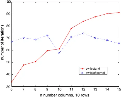
Both, the standard EW-TLS method (defined with the right kernel (16)) and the adapted EW-TLS method (14) are applied toD, described in Example 1, in order to find the best low rank r= 2 approximation matrixDˆ ofD. For everyn, the mean value of the number of iterations over the 100 runs is of interest and is visualized inFig. 1. We expected that in the case ofm≥n the number of iterations needed to compute the standard EW-TLS
6 7 8 9 10 11 12 13 14 15 30
40 50 60 70 80 90 100
n number columns, 10 rows
number of iterations
[image:4.595.321.553.536.722.2]ewtlsstand ewtlsleftkernel
solution would be less than the number of iterations needed to compute the adapted EW-TLS solution, and the other way around. The reason for this is that representations (3) and (5) lead to a different number of parameters. Fewer optimization variables result in less computations per iteration as well as in fewer iteration steps. Thus, by solving problem (1) it is important to use a representation of the rank constraint rank(Dˆ)≤r that leads to as few as possible optimization variables. From Fig. 1, it is clear that a smaller number of iterations is needed to compute the adapted EW-TLS solution form<n. Indeed, the average number of iterations depends on the number of parameters in the optimization problem to solve.
Example 2. The simulated data set contained spectra from 10 samples of three-component mixtures. The concentration of each component in each of the 10 mixtures had a value between 0 and 1 from a uniform random number distribution. The spectral profiles of the three components were Gaussian with a standard deviation of 20 nm and maximum molar absorptivities at 480 nm, 500 nm and 520 nm, respectively. Pure spectral vectors were generated between 400 nm and 600 nm at 20 nm intervals. The noise-free data matrix D0 was calculated by multiplying the 10 × 3 matrix of concentrations by the 3 × 11 matrix of pure component spectra. To add a noise matrixΔDof correlated measurement errors to the noise-free matrixD0,first a 10 × 11 matrix D′ of uncorrelated measurement errors was generated. The matrix of the measurement standard deviations corresponding to this 10 × 11 matrix is determined by generating a 10 × 11 matrix of uniformly distributed random numbers between 0 and 0.01. This ensures that there is no pattern in the standard deviation matrix. Now, the 10 × 11 matrix of uncorrelated measurement errors D′ is generated by taking a 10 × 11 random matrix with normally distributed elements (with Matlab's randn) and multiplying this matrix, element-wise, by the standard deviation matrix. To introduce correlations among the errors within the rows, the rows of matrixD′were filtered using a 1 × 5 moving average digital filter (see Ref. [2, Eqs. (34) (35) (36)] for the definition) to construct the correlated error matrix ΔD. This error matrixΔDwas added to the noise-free partD0in order to complete the noisy data matrixD=D0+ΔD of size 10 × 11.
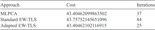
To the simulated data set described in Example 2 we have applied the MLPCA algorithm and the EW-TLS algorithms. All the algorithms start from the same initial approximation, the truncated SVD solution. After the algorithms reached their local minimum, we compared the final cost which is defined by vec⊺(D−Dˆ)W−1vec(D−Dˆ) for each algorithm and the number of iterations needed to converge to their local minimum. The results are presented in Table 1. From the
table it is clear that the adapted EW-TLS algorithm needs the fewest number of iterations for the case when the data matrix has size m×n, m≤n, and only row-wise correlated measure-ment errors.
In order to draw general conclusions about the right choice of algorithms to solve specific problems in chemometrics and other application fields, we created a simulation example, Example 3, which contains data matrices of size m×n with m<n, m>nor m=n. All the data matrices have measurement errors which are only correlated among the rows.
Example 3. The simulated data set containedm×nmatricesD, form= 6, 7,…, 13 andn= 20−m. The noise-free data matrixD0 of rankrwas calculated by multiplying an arbitrarym×rmatrix by an arbitraryr×nmatrix. The desired rankrwas varied from 1 to 4. For each combination of m and r, 50 independently generated data matricesDwere generated as follows. First, an m×n matrix D′ of uncorrelated measurement errors was generated. The matrix of the measurement standard deviations corresponding to thism×nmatrix is determined by generating an m×n matrix of uniformly distributed random numbers between 0 and 0.01. This ensures that there is no pattern in the standard deviation matrix. Now, them×nmatrix of uncorrelated measurement errorsD′is generated by taking anm×nrandom matrix with normally distributed elements (with Matlab's randn) and multiplying this matrix, element-wise, by the standard deviation matrix. To introduce correlations among the errors within the rows, the rows of matrixD′were filtered using a 1 × 5 moving average digital filter (see Ref. [2, Eqs. (34) (35) (36)] for the definition) to construct the correlated error matrixΔD. This error matrixΔDwas added to the noise-free partD0in order to complete the noisy data matrixD=D0+ΔD of sizem×n.
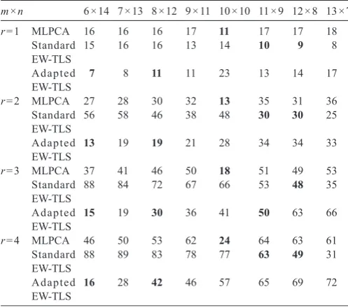
We have applied the MLPCA algorithm and the two EW-TLS algorithms to each of the data matricesDof the data set described in Example 3. The three algorithms were run from equivalent initial approximations obtained via the SVDs and the stopping criteria were set to the same tolerance. In all the runs, the same solution was found. As expected, the average number of iterations depends on the number of optimization parameters: the fewer the optimization variables, the fewer the average number of iterations for convergence. Numerical results are shown inTable 2. The table shows the number of iterations for each algorithm and for the differentm, nandr.
From the table it is clear that the adapted EW-TLS algorithm needs the fewest number of iterations for the case when the data matrix has sizem×nwithm<nand the measurement errors are only row-wise correlated. When m>n, the standard EW-TLS algorithm converges to the right solution within the fewest number of iterations. For square matrices with m=n, the MLPCA algorithm seems to converge in the fewest number of iterations.
[image:5.595.32.284.702.752.2]Nevertheless, in order to draw general conclusions about the right method of choice for a specific problem in chemometrics, besides the number of iterations, we also need to take into account the number of floating point operations (flops) per iteration for each of the algorithms discussed. The MLPCA Table 1
MLPCA and EW-TLS applied to the chemical data set described in Example 2
Approach Cost Iterations
MLPCA 43.40462099863502 37
Standard EW-TLS 43.75752145651096 84
algorithm is dominated by an SVD, whose computational cost is of the order of 4m2n+ 8mn2+ 9n3 for an m×n matrix. We obtained the following theoretical number of flops for minimizing the cost function (step 3) in the adapted EW-TLS algorithm, Algorithm 1: 2mn(m−r) + (m−r)2+mn2(m−r)2+ 2/ 3n3(m−r)3+n2(m−r)2+n(m−r). The theoretical number of flops for minimizing the cost functionf, expressed in (21), in the standard EW-TLS algorithm is of the orderm(2n(n−r) +n2(n− r) +n(n−r)2+ 2/3(n−r)3+ (n−r)2+ (n−r)). Given the iterative nature of the algorithms, the total number of flops is a multiple of the flops necessary to execute one iteration. Based on the number of iterations given inTable 2and the theoretical number of flops per iteration, we computed the total number of flops for each algorithm and for the different sizes ofm,n and r. The results are shown in Table 3. By underlining the number of iterations in the table, we emphasize which algorithm has the fewest computational load for the specific choices ofm,nandr. We clearly see the computational advantage of the adapted EW-TLS algorithm for the cases of m≪n and r> 2 and the computational advantage of the standard EW-TLS algorithm for
the case whenm》n. The standard EW-TLS algorithm seems to behave better. The reason for this is that we could not avoid the Kronecker product in the adapted TLS algorithm. The EW-TLS algorithms are only developed for cases of row-wise correlated measurement errors. So, for more general cases of measurement correlations the MLPCA algorithm should still be the method of choice.
Based on this experiment, we can conclude that the EW-TLS-like algorithms can indeed be nice alternatives to the MLPCA algorithm for the specific cases of row-wise correlated measurement errors and data matrices which are far from squared. Moreover, in paper[1]we showed that for uncorrelated measurement errors with equal row variances the GTLS algorithm performs best and that the standard EW-TLS algorithm is also useful for cases where the measurement errors have unequal row variances. We refer to paper [1]for further explanation.
5. Conclusion
In order to make the EW-TLS method useful for problems in chemometrics, we have derived an adapted version of this EW-TLS method. For the case when the data matrix D has much more columns than rows and only correlated measurement errors within the rows, we have presented an algorithm to compute the best low rank matrix approximation of D. Moreover, we have compared this new algorithm with the standard EW-TLS algorithm and the MLPCA algorithm in convergence behaviour on chemical data. It can be concluded that the EW-TLS-like algorithms are nice alternatives to the MLPCA algorithm for the specific cases of row-wise correlated measurement errors and data matrices which are far from squared. For more general cases of correlations between the measurements the MLPCA algorithm should still be the method of choice.
Acknowledgements
[image:6.595.42.291.104.324.2]Prof. Dr. Sabine Van Huffel is a full professor, Dr. Ivan Markovsky is a postdoctoral researcher and Mieke Schuermans is a research assistant at the Katholieke Universiteit Leuven, Belgium. Our research is supported by
Table 2
The number of iterations of the MLPCA and the EW-TLS algorithms by applying them to the chemical data set described in Example 3
m×n 6 × 14 7 × 13 8 × 12 9 × 11 10 × 10 11 × 9 12 × 8 13 × 7
r= 1 MLPCA 16 16 16 17 11 17 17 18
Standard EW-TLS
15 16 16 13 14 10 9 8
A d a p t e d EW-TLS
7 8 11 11 23 13 14 17
r= 2 MLPCA 27 28 30 32 13 35 31 36
Standard EW-TLS
56 58 46 38 48 30 30 25
A d a p t e d EW-TLS
13 19 19 21 28 34 34 33
r= 3 MLPCA 37 41 46 50 18 51 49 53
Standard EW-TLS
88 84 72 67 66 53 48 35
A d a p t e d EW-TLS
15 19 30 36 41 50 63 66
r= 4 MLPCA 46 50 53 62 24 64 63 61
Standard EW-TLS
88 89 83 78 77 63 49 31
A d a p t e d EW-TLS
16 28 42 46 57 65 69 72
Table 3
The total number of flops of the MLPCA and the EW-TLS algorithms by applying them to the chemical data set described in Example 3
m×n 6 × 14 7 × 13 8 × 12 9 × 11 10 × 10 11 × 9 12 × 8 13 × 7
r= 1 MLPCA 577,920 508,560 445,440 412,335 231,000 306,765 261,120 232,470
Standard EW-TLS 623,220 618,240 552,870 386,880 345,240 195,950 133,560 84,864
Adapted EW-TLS 1,847,300 2,930,000 5,061,287 5,868,400 13,272,633 7,609,810 7,802,300 8,437,644
r= 2 MLPCA 975,240 889,980 835,200 776,160 273,000 631,575 476,160 464,940
Standard EW-TLS 2,020,032 1,923,400 1,345,700 941,868 966,400 468,160 343,440 196,080
Adapted EW-TLS 1,817,100 4,139,800 5,638,212 7,668,304 11,577,000 14,788,980 14,506,000 12,855,524
r= 3 MLPCA 1,336,440 1,303,185 1,280,640 1,212,750 378,000 920,295 752,640 684,495
Standard EW-TLS 2,733,632 2,367,680 1,762,560 1,363,584 1,065,680 643,632 410,880 194,130
Adapted EW-TLS 934,425 2,207,200 5,323,350 8,514,500 11,648,000 15,638,000 20,040,615 19,751,000
r= 4 MLPCA 1,661,520 1,589,250 1,475,520 1,503,810 504,000 1,154,880 967,680 787,815
Standard EW-TLS 2,332,000 2,108,232 1,676,800 1,280,916 974,820 577500 300,272 113,646
[image:6.595.41.565.610.752.2]the Research Council KUL: GOA-AMBioRICS, several PhD/postdoc and fellow grants;
the Flemish Government: FWO: PhD/postdoc grants, projects, G.0270.02 (nonlinear Lp approximation), G.0360.05 (EEG, Epileptic), research communities (ICCoS, ANMMM);
the IWT: PhD Grants,
the Belgian Federal Government: IUAP V-22 (2002–2006): Dynamical Systems and Control: Computation, Identifica-tion and Modeling;
the EU: BIOPATTERN (FP6-2002-IST 508803), ETU-MOUR (FP6-2002-LIFESCIHEALTH 503094).
References
[1] M. Schuermans, I. Markovsky, P.D. Wentzell, S. Van Huffel, On the equivalence between total least squares and maximum likelihood PCA, Anal. Chim. Acta 544 (2005) 254–267.
[2] P.D. Wentzell, D.T. Andrews, D.C. Hamilton, K. Faber, B.R. Kowalski, Maximum likelihood principal component analysis, J. Chemom. 11 (1997) 339–366.
[3] P.D. Wentzell, M.T. Lohnes, Maximum likelihood principal component analysis with correlated measurement errors: theoretical and practical considerations, Chemometr. Intell. Lab. Syst. 45 (1999) 65–85.
[4] A. Premoli, M.L. Rastello, The parametric quadratic form method for solving problems with element-wise weighting, in: S. Van Huffel, P. Lemmerling (Eds.), Total least Squares and Errors-In-Variables Modeling: Analysis, Algorithms and Applications, Kluwer, 2002, pp. 67–76. [5] I. Markovsky, M.L. Rastello, A. Premoli, A. Kukush, S. Van Huffel, The
element-wise weighted total least squares problem, Comp. Stat. Data Anal. 50 (1) (2005) 181–209.