A nonparametric characteristics model of the demand for milk

A nonparametric characteristics model of the

demand for milk.

Laura M. Andersen*,

Laura Blow**,

Martin Browning***

Ian Crawford**

* AKF, Copenhagen;

** Institute for Fiscal Studies, London.

*** CAM, University of Copenhagen;

July 31, 2003

Abstract

Characteristics models in demand analysis capture the idea that people value goods not for the commodity itself but for the character-istics (or attributes) or embodied in the good. For example, agents may care about the fat content and the taste of different sorts of milk but not the actual type of milk. When we have fewer characteristics than types of good the theory imposes restrictions on observables.

We present a revealed preference characteristics model analysis of the demand for milk in Denmark.

1

Introduction.

We present an analysis of the demand for milk using a characteristics model in which agents value different types of milk for their characteristics (at-tributes) such as fat content, whether the milk is produced under envi-ronmentally friendly conditions (‘oko’ to use the Danish abbreviation) and taste. In this paper we consider only linear characteristics models. We de-velop Afriat-Varian style revealed preference tests for linear characteristics models that obviate the need for assuming a particular functional form for preferences. The principal questions we address are:

• are the data on milk prices and demand nonparametrically consistent with a linear characteristics model with a known technology?

• as well as the characteristics mentioned above, are other (latent) at-tributes also needed to rationalise the data?

• if the data are not consistent with a known technology, are they con-sistent with any non-trivial linear characteristics model?1

• if the data can be rationalised with a linear characteristics model, what are the implied bounds on the willingness to pay for a characteristic such as ‘oko’ ? Here we can make a distinction between the market valuation and the valuation for particular households.

• can a revealed preference analysis yield bounds on the value of a new market good that bundles attributes in some way that has not previ-ously been offered?

Milk is a particularly simple commodity to model since it is non-durable, non-storable (so that there is no inventory problem to deal with), absolutely homogeneous within milk types and we can observe some (or even all) of the characteristics in our data. Thus milk is one of the simplest commodities we could think of modelling (another is eggs, as in the classic paper in the field, Gorman (1980)). Despite this simplicity we shall see that important modelling and substantive issues arise. It is our hope that highlighting these for such a simple commodity will be useful for modelling goods such as soap powder, cars and personal computers.

The empirical analysis uses an unusual data set in which we have the records of purchases of milk (and other goods) for a large number of Danish households over several years (a maximum of 208 weeks for some house-holds). We conduct separate analyses for each household so that we do not have to model between household heterogeneity explicitly.2 Since so much of the subsequent analysis is motivated by the nature of our data, in the next section we present an detailed description of the data.

In the third section we consider the analysis of demand data using re-vealed preference techniques. A necessary condition for being able to ratio-nalise demand behaviour with a characteristics model is that the data satisfy the Generalised Axiom of Revealed Preference (GARP); see Varian (1982). If the data do pass GARP we can then ask whether the data are also con-sistent with the existence of a non-trivial linear characteristics model. The analysis is conducted for two cases; the first in which we know the linear technology (and all characteristics are observed) and the second in which we do not know the technology. Additionally we discuss one way to allow for measurement errors in prices for RP type tests.

1_{As we discuss below, a non-trivial characteristics model is one in which there are fewer}

characteristics than market goods.

2_{Or, rather, we deal with heterogeneity by allowing that preferences might be}

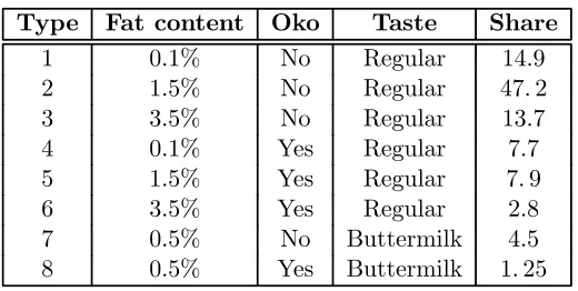
Type Fat content Oko Taste Share

1 0.1% No Regular 14.9

2 1.5% No Regular 47.2

3 3.5% No Regular 13.7

4 0.1% Yes Regular 7.7

5 1.5% Yes Regular 7.9

6 3.5% Yes Regular 2.8

7 0.5% No Buttermilk 4.5 8 0.5% Yes Buttermilk 1.25

Table 1: Types of milk

2

A

fi

rst look at the data.

2.1

The market for milk in Denmark.

We present a description of the milk market in Denmark during our sample period. This will include a discussion of the types of milk and the marketing structure. Discuss our sample period with mention of the introduction of ’mini-milk’ in thefinal year. Detailed description of how prices are set.

2.2

A description of the price data.

Describe how the data are collected.

For each household, daily records of expenditures (in Danish Kroner) and the quantity bought (in liters) of various types of milk are recorded. The types are differentiated by fat content, whether the milk is produced under environmentally congenial conditions (‘oko’) and taste. Table 1 records the characteristics of the eight types that we work with. We also record the market shares for the different types (these are derived for our total sample).3 As can be seen 75% of milk purchases are for regular non-oko milk. For oko milks, low fat is relatively popular (as compared to non-oko milk). We construct weekly unit values for each type of milk and each of nine regions 4 _{by dividing the weekly expenditure on that type of milk by all households}

in our survey in that region by the weekly quantity in the region. We shall refer to these week-region specific unit values as prices; note that these are absolute prices and are not deflated by any general price index. We have a number of missing values in our price data because no one in our sample bought that particular type of milk in that region and week. Table A1 in the

3

We exclude a small number of milk purchases that are not categorised and we also excludeflavoured milk.

4

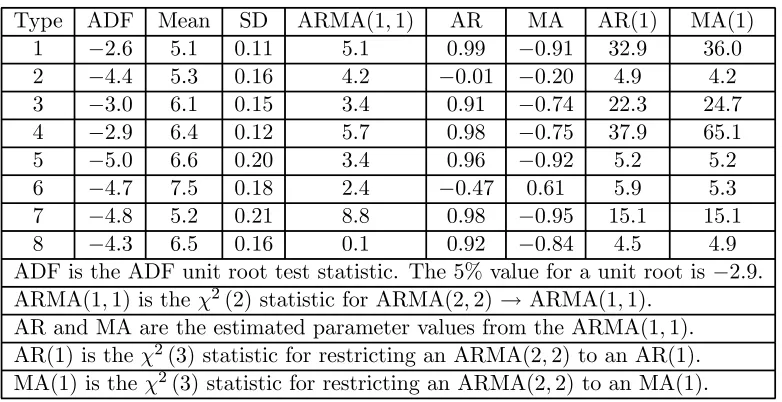
Type ADF Mean SD ARMA(1,1) AR MA AR(1) MA(1) 1 ₋2.6 5.1 0.11 5.1 0.99 ₋0.91 32.9 36.0 2 ₋4.4 5.3 0.16 4.2 ₋0.01 ₋0.20 4.9 4.2 3 ₋3.0 6.1 0.15 3.4 0.91 ₋0.74 22.3 24.7 4 ₋2.9 6.4 0.12 5.7 0.98 ₋0.75 37.9 65.1 5 ₋5.0 6.6 0.20 3.4 0.96 ₋0.92 5.2 5.2 6 ₋4.7 7.5 0.18 2.4 ₋0.47 0.61 5.9 5.3 7 ₋4.8 5.2 0.21 8.8 0.98 ₋0.95 15.1 15.1 8 ₋4.3 6.5 0.16 0.1 0.92 ₋0.84 4.5 4.9 ADF is the ADF unit root test statistic. The 5%value for a unit root is₋2.9. ARMA(1,1)is the χ2(2)statistic for ARMA(2,2)_→ARMA(1,1).

AR and MA are the estimated parameter values from the ARMA(1,1). AR(1) is theχ2_{(3)statistic for restricting an ARMA(2,2)to an AR(1).}

MA(1) is theχ2_{(3)statistic for restricting an ARMA(2,2)to an MA(1).}

Table 2: Price statistics

Appendix gives the number of weeks in which we do not observe a particular price for a particular region. We have very few observations in regions 3 (South Zealand) and5 (Bornholm) so we drop these from our analysis. We choose to impute missing prices for the remaining missing prices using a simple interpolation scheme; details are given in the Appendix.

Since the prices and their properties play an important role in the analy-sis below we present here a time series analyanaly-sis of the prices for one region (Copenhagen). For this region we do not have any missing values for any prices. Figure 1 presents the plots for 208 periods (1997.1 to 2000.52) for milk types 2, 3 and 5. The y-axis gives the price per liter in Danish Kroner (about 7 kroner to one Euro). The first feature of this figure is that there is a clear (upwards) break in prices for types 1 and 2 in weeks 15/16 and 194/195. This break is also seen in all of the other non-oko price series but not in any of the oko milk price series. In some of our analysis below it is convenient to work with stationary series, so we restrict attention to weeks 16 to 194 (a total of 179 time periods). In our demand analysis we use the whole sample since the discrete, persistent and exogenous change in the rel-ative price of oko milk obviously helps the identification of price effects. On the restricted period there is no visual evidence of a time trend in absolute prices over the 179 weeks of the sample; below we shall present formal tests for stationarity. The other important feature of the graphs is that higher fat milk is more expensive (compare types 1 and 2) and oko milk is more expensive (compare types 2 and 5). To supplement this visual analysis, we present some statistics for the eight price series in Table 2. milk).

from weeks 16 to 194.5 Although types 1 and 4 are marginal we shall proceed as though none of series has a unit root. Given this, we present means and standard deviations in columns 2 and 3. The means show that higher fat content milks cost more (ceteris paribus) as does oko milk. The differences between the mean price for non-oko and the comparable oko variety are all about 1.3 Kroner per liter. The other columns of Table 2 examine the univariate process that each price series follows. We start with an ARMA(2,2) with Gaussian errors. We then test for restricting this to an ARMA(1,1). The results for this test are given in column4; mostly we do not reject the restrictions. Thefinal two columns give the test statistics for restricting the processes to being even simpler than the ARMA(1,1). As can be seen, we reject these simpler models in most cases. Accepting that a common model of an ARMA(1,1)is appropriate, we present the parameter estimates in the columns headed AR and MA. One major surprise from this analysis is how different the processes are. For example, the price for regular 1.5% milk (type 2) displays no autoregressive component and only a small and negative MA component. On the other hand, regular0.1% milk (type 3) seems to have an autoregressive parameter that is almost unity and a very large and negative MA component.

In revealed preference analysis only relative prices matter. Infigure 2 we present the path of the relative price of type 5 (medium fat, oko) milk to the price of type 2 milk (medium fat, non-oko) milk. This displays considerable variability with a premium for oko of between10%and 35%(in the middle periods). This high variability is of considerable interest for the identification of price effects in a model that assumes intertemporal additivity but we must, of course, allow that some of it may be due to demand shocks.

2.3

A description of the quantity data.

The prices given above are assumed common to all households in the partic-ular week and region. The purchases by households are, of course, specific to the household. Here we present an informal analysis of the demand patterns for a small number of households who are present in our sample for a large number of contiguous weeks. To minimise ’taste changes’ we also select on the household not having any change in household structure, except for the ageing of the members. Describe sample.

Graphs of ‘aggregate’ data. For a given region (Copenhagen) graph aggregate budget shares for non-oko and oko regular milks. Also graphs of three fat types for non-oko and oko. Finally buttermilk, non-oko and oko.

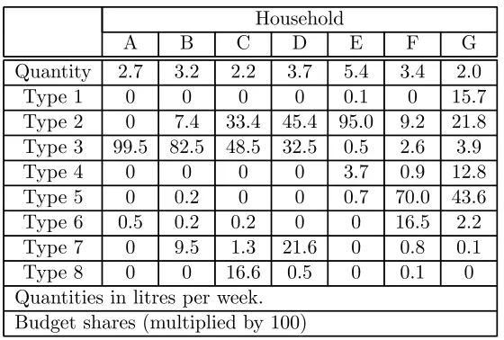
For illustrative purposes we consider seven households who are in our sample for almost 208 years and who consist of a married couple with no one else present during the whole data period. Table ??presents the mean

Household

A B C D E F G

Quantity 2.7 3.2 2.2 3.7 5.4 3.4 2.0

Type 1 0 0 0 0 0.1 0 15.7

Type 2 0 7.4 33.4 45.4 95.0 9.2 21.8 Type 3 99.5 82.5 48.5 32.5 0.5 2.6 3.9

Type 4 0 0 0 0 3.7 0.9 12.8

Type 5 0 0.2 0 0 0.7 70.0 43.6 Type 6 0.5 0.2 0.2 0 0 16.5 2.2 Type 7 0 9.5 1.3 21.6 0 0.8 0.1 Type 8 0 0 16.6 0.5 0 0.1 0 Quantities in litres per week.

Budget shares (multiplied by 100)

Table 3: Individual budget shares

budget shares (averaged over time) for the seven households for each of the eight goods.

Most obvious features:

• some households buy mostly one type of milk (A, B and E).

• lots of zeros over whole four years

• lots of heterogeneity

Figure ?? presents the time path of budget shares for types 2, 3 and 7 for household D. As can be seen, there seems to be a switch from type 3 to type 2 milk at around week 80. The research question is whether we can account for these changes assuming unchanging preferences.

The sample we work with is a sample of households who are present for at least 156 weeks of the 208 we consider and who live in the same region for the whole period. The numbers of such families are(133,112,62,136,60,59,66) for regions(1,2,4,6,7,8,9)respectively for a total of628households in all.

3

The linear characteristics model.

3.1

The basic framework.

we extend these conditions to the case where the data are generated by a utility maximising consumer whose preferences have the following structure:

u(q) =v(Aq) (1)

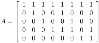
where A is a J _×K non-negative matrix with full row rank J < K. The J-vector z=Aq is a vector of characteristics or intermediate goods or at-tributes. To illustrate the use of characteristics consider our milk data. We have eight types of milk. One set of characteristics we could take are: (‘milk-iness’, 1.5% fat, 3.5% fat, oko, regular taste) so thatJ = 5.6 This gives the followingA matrix:

A= ⎡ ⎢ ⎢ ⎢ ⎢ ⎣

1 1 1 1 1 1 1 1 0 1 0 0 1 0 0 0 0 0 1 0 0 1 0 0 0 0 0 1 1 1 0 1 0 0 0 0 0 0 1 1

⎤ ⎥ ⎥ ⎥ ⎥ ⎦

This matrix has rank five. The technology is not unique, in the sense that BAis also a linear technology for any non-singular J_×J matrix; this cor-responds to a linear redefinition of the intermediate goods. For example, we could replace the first row with a vector so that the first characteris-tic is ‘0.1% fat’. If we assume that preferences are linear over fat content then we have only three characteristics, (fat,oko,taste) with following rank 3transformation matrix:

A=

⎡ ⎣

0.1 1.5 3.5 0.1 1.5 3.5 0.5 0.5 0 0 0 1 1 1 0 1 0 0 0 0 0 0 1 1

⎤ ⎦

It is important to test for this structure since if it is accepted we can put much tighter bounds on the market valuation of mini-milk (the new type of regular milk that was introduced with an0.5%fat content). Below we shall present tests for whether we can replace afive factor model by a three factor model.

4

The hedonic pricing model.

4.1

Known technology.

A particularly important special case of the linear characteristics model is when prices are such that the available characteristics for a fixed outlay on market goods all lie on a hyperplane; this is the hedonic pricing model. Figure ?? illustrates for a three good, two characteristics model. In the

6_{Note that buttermilk is different in both taste and fat content but we can only allow}

left hand panel we have that the available budget set is not linear and we do not have a hedonic model. In the right panel the price of good 2 has been increased until the boundary of the budget set is linear. The defining characteristic of a hedonic pricing model is that market prices are simply the weighted sums of the prices of the underlying shadow prices,πj_t:

pt=A0π˜t µ

µ_t λt

¶

=A0πt (2)

where theπ˜j_t’s areshadow prices for the characteristics.

We begin by considering the case in which the linear technology A is known. In this case the full set of characteristicszt=Aqt are also observed if market purchases are observed. From equation (2) we see that we need to find shadow prices πt such that pt = A0πt for all t. For each t this is a system of K equations in J < K unknowns so that a solution does not generally exist. The following gives the well-known condition for existence, where(A0_|pt) is the K_×(J+ 1) matrix of A0 and pt stacked horizontally.

Lemma 1 There exists aπtsatisfyingpt=A0πtif and only ifrank(A0|pt) = J. If this condition holds then πt is given uniquely by:

πt= ¡

AA0¢−1Apt (3)

Some remarks:

• It is important to recognise that given any A and pt we can always define πtuniquely in this way, but this πt will only satisfypt=A0πt exactly if the rank condition holds.

• Even if the rank condition holds,A is nonnegative and market prices are positive we may have πj_t < 0 for some j, t so that shadow prices may not always be positive.

• A result that is useful below is that:

rank¡A0_|pt¢=J _⇒A0¡AA0¢−1Apt=pt (4)

The implications of this for the revealed preference conditions are given by:

Proposition 2 If rank(A0_{|pt) = J for all t then {qt,pt} satisfies GARP}

if and only if _{zt,πt}satisfies GARP.

Proof. Suppose the rank condition holds and _{qt,pt} satisfies GARP.

GARP for _{qt,pt} implies:

(where we have, without loss of generality, taken a chain of length3,_{t, s, w_}). Given the rank condition we canfind unique shadow prices for period tthat satisfies pt = Aπt (and similarly for s and w). Substituting for market

prices this gives:

π0_tAqt_≥π0_tAqs andπ0_sAqs_≥π0_sAqw _⇒π0_wAqw_≤π0_wAqt (6)

so that:

π0_tzt≥π0tzs and π0szs≥π0szw ⇒π0wzw ≤π0wzt (7)

which is GARP on_{zt,πt}.

Conversely, for GARP on _{zt,πt} we examine inequalities such as:

π0_tzt≥π0tzs (8)

Substituting for zt and πt and using (4) this implies:

p0_tA0¡AA0¢−1Aqt≥p0tA0 ¡

AA0¢−1Aqs⇒pt0qt≥p0tqs (9)

so that GARP holds for _{qt,pt} if it holds for {zt,πt}.

Given these results we have a clear path for revealed preference testing for a characteristics model. First we test for GARP for the observed data

{qt,pt}. Clearly if this fails there is no utility model that rationalises the data. Strictly GARP tests for the milk group being a separable group. If the test fails we can attribute this to several reasons: the group is separable but the demand for milk products is not ‘rational’; the group is not separable (for example, we do not include substitutes such as other types of drink or other sources of calcium and fat); the group is separable but preferences for milk products change over time; the group is separable but preferences for milk products are not time separable (there are habits); the prices or quantities are measured with error. We shall return to some of these issues below. If the market data satisfy GARP, then we test for the rank condition. If this passes, then a characteristics model with this linear technology rationalises the data. If the demand data satisfy GARP but the prices fail the rank condition then we conclude that there is no characteristics model that rationalises the data

with the given linear technology . If this happens, two issues arise. First, we can ask: is there any linear technology that is consistent with the data? This is dealt with in the next sub-section. The second issue allows that prices might be measured with error.

4.2

Noisy prices.

Suppose that we assume that true prices do satisfy the rank condition in each period but that prices are measured with an additive error:

whereη_t is a serially uncorrelated vector process with zero mean and con-stant covariance matrixΣη. Let P be the K×T matrix of observed prices stacked horizontally. If we have more time periods than goods (T > K) then if η_t has a non-degenerate distribution, we will almost surely have rank(P) =K so that the exact rank condition of the previous section will never hold. One procedure in this case is to regress prices in periodton the transposed characteristics matrixA0 to give estimates of the shadow prices:

ˆ

πt= ¡

AA0¢−1Apt (11)

and then to define ‘predicted prices’:

ˆ

pt=A0πˆt=A0 ¡

AA0¢−1Apt (12)

If (and only if) the price vector in period t satisfies the rank condition of the previous subsection then ptˆ = pt (see equation (4)). Given predicted prices, the following gives a test for a characteristics model.

Proposition 3 The following are equivalent: (i) _{qt,ptˆ _} satisfies GARP

(iii)_{Aqt,πˆt} satisfies GARP

(ii) there is a characteristics model with linear technology A that ratio-nalises the data.

It is important to emphasise that GARP tests can pass for _{qt,ptˆ _} but fail for_{qt,pt}(and vice versa) unless the rank condition holds for each period. This framework can also be used to give the means of the shadow prices,

µ_π, and hence valuations for the different characteristics. The obvious esti-mator to take for the mean is:

¯

π =1

T X

ˆ

πt= ¡

AA0¢−1A1 T

X pt=

¡

AA0¢−1A¯p (13)

Under the stationarity assumption, this is a consistent estimator ofµ_π. Although the solution given in (11) is standard in the static factor analy-sis literature it ignores the time series structure of shadow and market prices. To take account of this, assume that shadow prices follow a stationaryfirst order vector autoregression:

πt= (I−B)µπ+Bπt−1+ut (14)

dynamic factor model; in this state space form it was introduced by Engle and Watson (1981). In our structure we have a fixed and small number of variables (K prices) and large T. Thus our structure is somewhat simpler than for dynamic factor models with large K and T (see, for example, Bai and Ng (2002)) or for models withK >> T, as in Stock and Watson (1998). Taking account of the time series structure will provide a lower variance estimator for the mean of the shadow prices. It will also facilitate testing for additional factors or an alternative characteristics structure without the need to use the tests for rank developed in, for example, Cragg and Don-aldson (1997). The obvious estimation procedure is to use Kalman filter based ML. An alternative is based on the reduced form of the state space representation. From the (lagged) measurement equations we have:

πt−1=

¡

AA0¢−1Apt₋1−

¡

AA0¢−1Aη_t−1

If we substitute the transition equations into the measurement equations and use this then we have the reduced form:

pt = A0(I−B)µπ+A0B ¡

AA0¢−1Apt−1

−A0B¡AA0¢−1Aη_t−1+η_t+A0ut (15)

so that prices follow a vector ARMA(1,1)(see Pena and Box (1987)):

pt=d+Cpt−1+vt+Θvt−1

This is consistent with the time series properties for prices found in section 2. From this framework we can derive predictions of shadow prices that are alternative to those derived from (11).

4.3

Additional latent attributes.

We can ask: given the technology described byA, do we need an additional (latent) attribute to adequately describe the evolution of prices?

4.4

Unknown linear technology.

Suppose that we have market data _{qt,pt_}t=1,..T that satisfy GARP and that prices and quantities are measured without error. We suspect that this may be rationalisable by a linear technology characteristics model but the form of the technology (and the number of characteristics) is unknown.7 Clearly if we allow for as many characteristics as goods (J = K) then we can always do this by settingA=IK. Thus we shall seek anon-trivial linear

characteristics model withJ < K.

7_{This clearly requires that characteristics are not observed by the analyst (otherwise we}

Proposition 4 Suppose the market data _{qt,pt} satisfy GARP. We can

find a non-trivial linear characteristics model that rationalises the data if and only if rank(P)< K .

Proof. Consider theK_×T matrix of pricesP and letrank(P) =J <

K. LetΠ be a J_×T row basis matrix forP (that is, every row ofP can be expressed as a linear combination of rows of Π). By definition Π has rank

J. Now consider the set of equations P =A0Π where A is aJ _×K matrix. By the definition of Π a solution A exists and is given by:

A=¡ΠΠ0¢−1ΠP0 (16)

Now take the characteristics model withzt=Aqt andπt as thet’th column

of Π (so that pt=A0πt). This satisfies the conditions of Proposition 1 and

hence we have found a linear characteristics model that rationalises the data. Conversely, suppose that there is a non-trivial linear characteristics model that rationalises the data. Suppose that this has J characteristics. Then proposition1 gives thatrank(A0_{|P) =J which implies thatrank(P)≤J <} K.

A number of remarks:

• Given GARP for a particular household, the condition for the existence and construction of a linear technology depends only on market prices that household faces and not on the market purchases.

• If we have fewer time periods than goods (T < K) then rank(P) _≤ T < Kso that we can alwaysfind a linear technology that rationalises the data if it satisfies GARP.

• There is nothing to ensure that all of the elements of A are non-negative even if all market prices are positive. We conjecture that there is some way to choose the row basis matrix so thatA is always non-negative. Consider, for example, the following technology with T = 7and K= 6:

P = ⎡ ⎢ ⎢ ⎢ ⎢ ⎢ ⎢ ⎣

1 2 3 4 5 4 5 2 2 2 3 5 5 5 1 2 3 4 5 4 5 1 2 2 3 4 4 5 1 2 3 4 5 4 5 3 4 4 6 9 9 10

⎤ ⎥ ⎥ ⎥ ⎥ ⎥ ⎥ ⎦ (17)

This has rank3. If we take a random row basis matrix then we always end up with at least one negative element in each row of A. On the other hand, if we take the row basis given by rows1,2 and4:

Π=

⎡ ⎣

1 2 3 4 5 4 5 2 2 2 3 5 5 5 1 2 2 3 4 4 5

⎤

we have:

A=

⎡ ⎣

1 0 1 0 1 0 0 1 0 0 0 1 0 0 0 1 0 1

⎤

⎦ (19)

which does satisfy our non-negativity restriction.

4.5

Noisy prices.

In general we will have many more periods than goods (T >> K) and any noise in observing prices will almost surely giverank(P) =K. On the other hand we might posit that ‘true’ pricesP∗ do have rank less than K . One informal check is to examine the eigenvalues of theK_×K matrixP P0. More acceptable would be to conduct a test on the rank ofP.

Use dynamic factor model to determine the number of factors and the form of the transformation matrixA.

5

Testing for a linear characteristics model.

5.1

Known technology.

The previous section dealt with testing for a hedonic pricing model and was concerned solely with market prices. In this section we move to a revealed preference analysis of individual demands. We provides tests for whether a time series of emands for a given agent can be rationalised by utility function that has a linear characetristics form given in equation (1) and reproduced eher for convenience:

u(q) =v(Aq) (20)

whereA is aJ_×K matrix with full row rank.

6

Conclusions.

References

[1] Bai, Jushan and Serena Ng (2002), “Determining the number of factors in approximate factor models”,Econometrica, 70(1), 191-222.

[2] Cragg, John and Stephen Donald (1997), “Inferring the rank of a ma-trix”,Journal of Econometrics, 76, 223-250.

[3] Gorman, W.M. (1980), “...”,Review of Economic Studies,

[4] Gregory, Alan, A. Head and J. Raynauld (1997), “Measuring world busi-ness cycles”, International Economic Review, 38, 677-701.

[6] Harvey, Andrew (1990), Forecasting, structural time series models and the Kalman filter, Cambridge University press, Cambridge.

[7] Pena, Daniel and George Box (1987), ”Identifying a simplifying structure in time series”,Journal of the American Statistical Association, 82, 836-843.

[8] Stock, James and Mark Watson (1998), “Diffusion indexes”, NBER Working Paper 6702.

A

Imputation of prices.

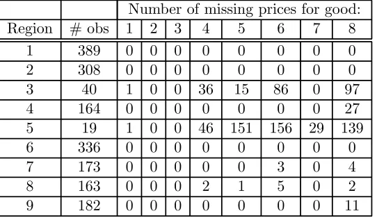
The following Table gives the mean number of households in each region per week and the number of missing values for prices. Note that prices are based on the full set of observations and not just those that are included in our final elected sample of households. We drop regions 3 and 5 since we have so few observations. For the other regions we have relatively few missing price values for types1to7 (11 out of a total of1456prices) so we simply use the simple interpolation scheme:

pi_r,t= 0.5_∗¡p_r,ti ₋₁+pi_r,t+1¢

wherer denotes region, idenotes the milk type andt is time. For the milk type 8which has44 missing values, we use??.

Number of missing prices for good: Region # obs 1 2 3 4 5 6 7 8

1 389 0 0 0 0 0 0 0 0

2 308 0 0 0 0 0 0 0 0

3 40 1 0 0 36 15 86 0 97

4 164 0 0 0 0 0 0 0 27

5 19 1 0 0 46 151 156 29 139

6 336 0 0 0 0 0 0 0 0

7 173 0 0 0 0 0 3 0 4

8 163 0 0 0 2 1 5 0 2

9 182 0 0 0 0 0 0 0 11

B

Figures.