Power-variance models for modelling rainfall

Peter K Dunn

_{and Neil White}

1 _{Department of Mathematics and Computing, University of Southern}

Queens-land, Q 4350, Australia

2 _{Emerging Technologies, Department of Primary Industries and Fisheries, PO}

Box 102 Toowoomba Q 4350, Australia

Abstract:Modelling rainfall presents difficulties: one is that rainfall is both con-tinuous and discrete. The discrete component corresponds to exactly zero rainfall. Some researchers circumvent this by using two models—one for determining the presence and absence of rainfall, another for the rainfall amount. Here, we use power-variance (Tweedie) generalized linear models, which can explictly model continuous data with exact zeros. We demonstrate there is a basis for using these models; that the parameters, in some cases, lend themselves to a useful interpre-tation; and show the models fit the data well using monthly rainfall data from Charleville. We then model Australian annual rainfall, and develop a contour map for the power-variance model index parameter.

Keywords: Tweedie model; rainfall; generalized linear model; power-variance models.

1

Introduction

2

Background

Generalized linear models (McCullagh & Nelder, 1989), orglms, have been

used for fitting models to climatological data such as rainfall by numerous researchers (for example, Coe & Stern, 1982; Stern & Coe, 1984; Chandler & Wheater, 2002). One difficulty is that rainfall data is continuous with exact zeros (when there is exactly no rainfall). Consequently, the mod-elling often consists of two stages: first, modmod-elling the presence or absence of rainfall using a binomial model (for example, Feuerverge, 1979; Chandler & Wheater, 2002); secondly, modelling the rainfall using a gamma distri-bution, a variation of a gamma distridistri-bution, or a combination of gamma distributions (for example, Allan & Haan, 1975; Stern & Coe, 1984; Wilks, 1999; Chandler & Wheater, 2002). Das (1955) and Wilks (1990) use a mod-ified gamma distribution to allow exact zeros to be modelled. In this paper, we demonstrate an attractive alternative using power-variance generalized linear models. A special case of the power-variance models, the Poisson-gamma models, are a convenient starting point.

The Poisson-gamma models can be developed as follows. Assume any pre-cipitation event igives an amount of precipitation Ri, and each Ri has a

gamma distribution Gam(−α, γ). (In this parameterization, the mean is −αγand variance−αγ2

.) The negative value forαis used to be consistent with that used elsewhere in this paper. Assume the number of precipitation events in any one day, say N, has a Poisson distribution (implying days with no precipitation events when N = 0.) The total daily precipitation,

Y, is the Poisson sum of the gamma random variables,

Y =R1+R2+· · ·+RN,

whereN has a Poisson distribution with meanλ.

An identical argument can be applied to monthly precipitation, when N

refers to the number of precipitation events in the month,Ri refers to the

precipitation recorded in those events, andY the total monthly precipita-tion. The generalization to longer time scales follows.

The distribution of total precipitation Y is deduced by working with cu-mulant generating functions (see Smyth, 1996), noting thatY givenN has the gamma distribution Gam(−N α, γ).

The resulting probability function is complicated, and cannot be written in closed form; see Dunn & Smyth (2005) for an infinite series expansion. Because of the relationship to the gamma and Poisson distributions, Smyth (1996) calls these distributions the Poisson-gamma distributions, the ter-minology adopted here.

Poisson-gamma models belong to the exponential dispersion model, oredm,

family of distributions (see Jørgensen, 1997).edms have density functions

or probability mass functions of the form

f(y;θ, φ) =a(y, φ) exp ₁

φ

yθ−κ(θ)

for suitable known functions κ() and a() (Jørgensen, 1997). The mean of the distribution is µ= ˙κ(θ) and the variance isφκ¨(θ). Since the mapping from θ to µ is invertible, write ¨κ(θ) =V(µ) for a suitable functionV(µ), called the variance function of theedm. The Poisson-gamma distributions

have variance functions of the form V(µ) =µp _{for some psuch that 1 <}

p < 2. More generally, edms exist for all values ofp outside the interval

(0,1) (Jørgensen, 1987). This family is called the power-variance family of distributions, or the Tweedie model family, because the underlying linear exponential families were first studied systematically by Tweedie (1946). The notation Y ∼ EDp(µ, φ) is used to indicate Y is distributed as a

Tweedieedmwith mean_µ, dispersion_φand variance function _V(_µ) =_µp.

Whenp≥2, the Tweedie models have support on the positive reals; indeed,

p= 2 corresponds to the gamma distribution. We concern ourselves with the casesp >1.

The relationship between the parameters of the Poisson and gamma distri-bution, and the edmnotation is

λ= 1

φ

µ2₋p

2−p, α=

2−p

1−p, τ =φ(p−1)µ

p−1

(2)

3

Fitting models

The Tweedie family is a three parameter family of distributions inµ (the mean),φ >0 (the dispersion parameter) andp. The estimation ofµfollows standard algorithms; see McCullagh & Nelder (1989) for details.

The maximum likelihood estimation of φ is more difficult; complicated algorithms are available for maximum likelihood estimation of φ(Dunn & Smyth, 2001; Dunn & Smyth, 2003). An alternative method of estimation is to use the mean deviance estimator of φ; this is closely related to using the saddlepoint approximation (see Jørgensen, 1997) in place of the true likelihood. Dunn & Smyth (2005) show this method may have difficulties for continuous data with exact zeros. In this paper, the maximum likelihood estimate ofφis used unless stated otherwise.

Estimating the maximum likelihood value of p is performed using a pro-file (log-) likelihood plot which requires the computation of the density. This is difficult, though computational programs are available (Dunn & Smyth, 2003). Here, we use the series expansion of the densities (Dunn & Smyth, 2005) to compute the log-likelihood. For a given fixed value of

p, maximum likelihood estimates ofµ and φare computed as above, and the log-likelihood computed. The value of pfor which the log-likelihood is maximized is chosen as the maximum likelihood value. Some examples are shown in the next section.

Nominal confidence intervals forpcan also be found, since 2 [logL(ˆp)−logL(p0)] has, asymptotically, aχ2

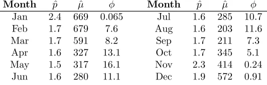
TABLE 1. Maximum likelihood estimates ofp,µandφfor fitting Poisson-gamma distributions to total monthly precipitation at Charleville.

Month _{pˆ µˆ φ}ˆ Month _{pˆ µˆ φ}ˆ

Jan 2.4 669 0.065 Jul 1.6 285 10.7 Feb 1.7 679 7.6 Aug 1.6 203 11.6 Mar 1.7 591 8.2 Sep 1.7 211 7.3 Apr 1.6 327 13.1 Oct 1.7 345 5.1 May 1.5 317 16.1 Nov 2.3 414 0.24

Jun 1.6 280 11.1 Dec 1.9 572 0.91

TABLE 2. The maximum likelihood estimates from Table 1 for Charleville, repa-rameterized in terms ofλ(the mean number of precipitation events per month),

γ (the shape of the rainfall gamma distribution) and −αγ (the amount of rain

per event). Note that for January and November, this interpretation is nonsense asp >2.

Month _λˆ _{ˆγ −ˆαγˆ} Month _λˆ _{ˆγ −ˆαγˆ}

Jan −2.6 871 −252 Jul 2.1 228 137 Feb 3.3 422 203 Aug 1.9 151 107 Mar 2.7 524 218 Sep 2.2 226 94 Apr 1.8 282 177 Oct 3.6 241 96 May 2.0 184 161 Nov −3.4 594 −123

Jun 2.3 162 120 Dec 27.5 343 20.8

4

Example

Consider the total monthly precipitation recorded at Charleville, Queens-land, Australia, from 1882 to 1994. Each month has 113 observations. Rain-fall was recorded every January, November and December; consequently,

1< p <2 for all other months. The maximum likelihood estimates ofµ,p

andφfor each month are shown in Table 1.

−2 −1 0 1 2 −5

0 5 10

April rainfall Deviance residuals

Theoretical Quantiles

Quantile Residuals

−2 −1 0 1 2 −2

−1 0 1 2 3

April rainfall

(Randomized) quantile residuals

Theoretical Quantiles

Quantile Residuals

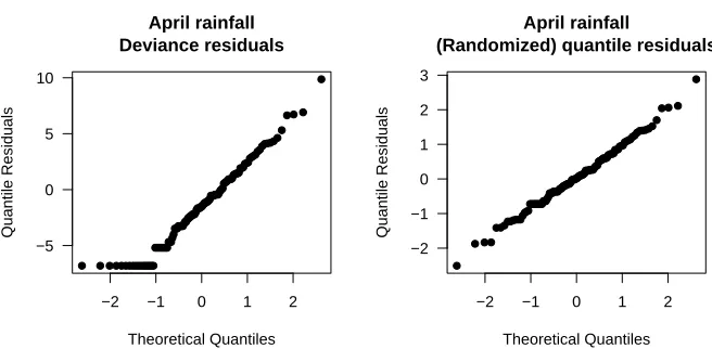
FIGURE 1. The QQ-plots from fitting a power-varianceglmto the April monthly

rainfall at Charleville. The quantile residuals indicate the model fits well; the deviance residuals are less conclusive.

5

Evaluation of models

To assess the quality of the fitted distributions, quantile residuals are best used (Dunn & Smyth, 1996). One feature of quantile residuals is they have an exact standard Normal distribution (apart from sampling error) pro-vided the correct distribution is used. This is true even for discrete distribu-tions, or distributions with a discrete component (like the Poisson-gamma distributions). In this case, the smallest necessary amount of randomisation is introduced, and replications of the residuals are recommended; any pat-tern not preserved across replications are then considered artefacts of the randomisation. One typical QQ-plot of these quantile residuals are shown in the right plot of Figure 1. In all cases, the plots show the distributions model the total monthly precipitation well. In contrast, using deviance residuals makes this decision difficult (see the left plot of Figure 1) as the residuals corresponding to exact zeros form distinct and distracting lines in the plots.

6

Contours for Australian rainfall stations

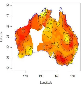
FIGURE 2. Contours for fitting the Poisson-gamma models to 591 randomly se-lected mainland Australia rainfall stations using the saddlepoint approximation.

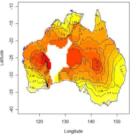
the automated process used here it provided usable estimates for only 375 of the rainfall stations considered. The series method, while substantially slower, was able to automatically estimatepfor 550 of the selected stations. Using the sgeostat kriging function with an exponential fit to the var-iogram, the contours of the index p are plotted in Figures 2 (using the saddlepoint approximation for estimation) and 3 (using the series expan-sion for estimation). The area in central Australia is sparsely populated with few meteorological stations. The variogram was undertaken using a maximum distance between pairs of 3◦ _{(approximately 300 km).}

FIGURE 3. Contours for fitting the Poisson-gamma models to 591 randomly selected mainland Australia rainfall stations using an accurate series expansion to evaluation the likelihood.

1 < p < 2, implying many years with no rainfall. In contrast, the more

accurate (but slower) series method ensuresp >2.

References

Allan, D.M., and Haan, C.T. (1975). Stochastic simulation of daily rain-fall. Research Report No. 82, Water Resources Institute, University of Kentucky.

Chandler, R.E., and Wheater, H.S. (2002). Analysis of rainfall variability using generalized linear models: a case study from the west of Ireland.

Coe, R., and Stern, R.D. (1982). Fitting models to daily rainfall.Journal of the Applied Meteorology. 21_{, 1024–1031.}

Das, S.C. (1955). The fitting of truncated Type III curves to daily rainfall data. Australian Journal of Physics, 8_{, 298–304.}

Dunn, P.K., and Smyth, G.K. (2005). Series evaluation of Tweedie expo-nential dispersion models.Statistics and Computing, to appear.

Dunn, P.K., and Smyth, G.K. (1996). Randomized quantile residuals. Jour-nal of ComputatioJour-nal and Graphical Statistics.5_{, 236–244.}

Dunn, P.K., and Smyth, G.K. (2001). Tweedie family densities: methods of evaluation. In:New Trends in Statistical Modelling: Proceedings of the 16th International Workshop on Statistical Modelling. 155–162, Odense, Denmark.

Feuerverger, A. (1979). On some methods of analysis for weather experi-ments.Biometrika.66_{, 655–658.}

Jørgensen, B. (1997).The theory of dispersion models. London: Chapman and Hall.

Jørgensen, B. (1987). Exponential dispersion models (with discussion). Jour-nal of the Royal Statistical Society, Series B. 49_{, 127–162.}

McCullagh, P., and Nelder, J.A. (1989).Generalized linear models, second edition. London: Chapman and Hall.

Stern, R.D., and Coe, R. (1984). A model fitting analysis of daily rainfall data (with discussion). Journal of the Royal Statistical Society, Se-ries A.147_{, 1–34.}

Smyth, G.K. (1996). Regression analysis of quantity data with exact ze-roes. In: Proceedings of the Second Australia–Japan Workshop on Stochastic Models in Engineering, Technology and Management. 572– 580, Technology Management Centre, University of Queensland, Bris-bane.

Tweedie, M.C.K. (1946). The regression of the sample variance on the sam-ple mean.Journal of the London Mathematical Society.21_{, 22–28.}

Wilks, D.S. (1990). Maximum likelihood estimation for the gamma distri-bution using data containing zeros.Journal of Climate.3_{, 1495–1501.}