White Rose Research Online URL for this paper:
http://eprints.whiterose.ac.uk/74770/
Monograph:
Giagkiozis, I. and Fleming, P.J. (2012) Methods for many-objective optimization: an
analysis. Research Report. ACSE Research Report no. 1030 . Automatic Control and
Systems Engineering, University of Sheffield
[email protected] https://eprints.whiterose.ac.uk/ Reuse
Unless indicated otherwise, fulltext items are protected by copyright with all rights reserved. The copyright exception in section 29 of the Copyright, Designs and Patents Act 1988 allows the making of a single copy solely for the purpose of non-commercial research or private study within the limits of fair dealing. The publisher or other rights-holder may allow further reproduction and re-use of this version - refer to the White Rose Research Online record for this item. Where records identify the publisher as the copyright holder, users can verify any specific terms of use on the publisher’s website.
Takedown
If you consider content in White Rose Research Online to be in breach of UK law, please notify us by
Methods for Many-Objective Optimization: An
Analysis
Ioannis Giagkiozis, and Peter J. Fleming
Department of Automatic Control and Systems Engineering
The University of Sheffield
Research Report No. 1030
November 2012
Abstract—Decomposition-based methods are often cited as the
solution to problems related with many-objective optimization. Decomposition-based methods employ a scalarizing function to reduce a many-objective problem into a set of single objective problems, which upon solution yields a good approximation of the set of optimal solutions. This set is commonly referred to as Pareto front. In this work we explore the implications of using decomposition-based methods over Pareto-based methods from a probabilistic point of view. Namely, we investigate whether there is an advantage of using a decomposition-based method, for example using the Chebyshev scalarizing function, over Pareto-based methods.
Index Terms—Many-Objective optimization, Chebychev
de-composition, Pareto-based methods, Decomposition-based meth-ods
I. INTRODUCTION
A
traditional classification of optimisation problems has been their separation into linear and nonlinear problems [1]. However, this ignores a large body of research in convex programming, which is a special class of methods that apply to a subclass of nonlinear optimisation problems, for which a solution can be obtained with relative ease, even for relatively large scale problems [2]. Therefore a more relevant distinction of optimisation problems would be their classification based on convexity. This is so because this distinction will radically impact the approach used in solving such problems and the expected quality of the produced solutions. In the fortunate case that a problem can be expressed in a convex form, then for all practical purposes it can almost be considered as solved. Furthermore the solution obtained for convex problems is guaranteed to be the global optimum, however it is not necessarily unique. Namely, a solution obtained for a convex program is the global minimum (maximum) for a minimi-sation (maximiminimi-sation) problem. Also such a solution can be obtained quite efficiently [2]. These facts strongly motivate the additional effort required to attempt to identify whether a problem is convex. However the process of identifying a convex problem is non-trivial and is further complicated by the fact that different formulations can be more difficult to solve [2].The authors are with the Department of Automatic Control and Systems Engineering, University of Sheffield, Sheffield, UK, S1 3JD.
E-mail: [email protected] URL: http://ioannis-giagkiozis.staff.shef.ac.uk
For nonconvex problems, guarantees about the obtained solution can only be given when an exhaustive search is performed. That is, only if the entire domain of definition of the objective function is explored. Naturally such a task can very easily become unmanageable. However once the fact that a problem is nonconvex is established, there are several metaheuristics1 that can be employed to obtain a
solution. Some examples of metaheuristics, often referred to as evolutionary algorithms (EAs) in the literature are, genetic algorithms (GAs) [3], [4], evolution strategies (ES) [5], differential evolution (DE) [6] particle swarm optimisation (PSO) [7], [8] and others [9]–[11].
Although a solution produced by any of the aforementioned methods will most likely be suboptimal, metaheuristics per-form well in practice. Meaning that compared to the alternative of using random search [12], [13], which has the property of asymptotical convergence [14], EAs in practice, converge
faster to the neighbourhood of optimal solutions for a number
of problems [15]–[18]. Of course, this does not imply that EAs are superior to random search for all problems. The implication is that if domain knowledge is exploited then EAs can be a very effective [19], especially in light of the fact that even convex problems turn into nonconvex at the slightest provocation. An example of this phenomenon is seen in machine learning, where kernel-based learning algorithms that have a shallow architecture, namely a single layer of kernels for which the weights are to be determined, are linear in the parameters and produce convex problems. However, such architectures seem to be inefficient for certain tasks while
deep architectures, namely architectures with several layers
of kernels, can learn more complex tasks more efficiently, however the estimation of their parameters (learning) is non-convex [20]. Such examples serve as feedback to practitioners not to become overly dependent on a particular method, but instead, carefully investigate the nature of the problem so as to select the optimal approach for its solution, a process that is nonconvex in itself.
Another important classification is the separation of optimi-sation problems into single-objective, that is problems where the objective function is a mapping of the type f :Cn →C,
and, multi-objective whereby the objective function mapping
1An algorithmic framework of heuristic optimisation algorithms. Heuristic
has the following form2 f : Cn →Ck. This classification is
important because in the latter case, there is no obvious or unique way to induce a complete ordering for nonconvex [21, pp. 113], [1, pp. 61] as well as for convex problems [2, pp. 174]. Without order a direction of search cannot be established. This is a well known issue in multi-objective optimisation and has been addressed to varying degrees of success by several researchers in the field of mathematical programming [21]–[23] and more recently in evolutionary computation [4], [24], [25]. In general there are two approaches employed to resolve this issue: Pareto-based and decomposition-based methods. In both methodologies and assuming, the a posteriori preference articulation paradigm [1, pp. 63] is employed, the relative importance of the objectives is unknown. In the case that preference information is given by the decision maker (DM), then using a decomposition method to combine the scalar objective functions can be used, see Section IV. An alternative is to distill the preference information given by the decision maker in a utility function, however this requires extensive knowledge of the problem structure and does not guarantee that its solutions will be Pareto optimal [21, pp. 62]. Pareto-based methods use the Pareto-dominance relations [1] to induce partial ordering in the objective space.
Decomposition-based methods have been predominantly used in mathematical programming [1], [2]. These methods use scalarising functions to decompose a multi-objective prob-lem into several single objective subprobprob-lems. These subprob-lems are defined with the help of weighting vectors. The weighting vectors are k-dimensional vectors with positive3 components whose sum is equal to one. The location on the Pareto front that each subproblem tends to converge, depends on the choice of weighting vectors and the scalarizing function of choice. Therefore, to control the final distribution of solutions on the Pareto front the set of weighting vectors must be carefully selected for the entire Pareto front to be covered.
Many-objective problems are an important subclass of multi-objective problems that have more than 3 objectives, with applications in control and aerospace [9], [26]. However, as many authors point out, Pareto-based evolutionary algo-rithms are facing difficulties for many-objective problems for a number of reasons. For example, for increasing number of dimensions the number of incomparable solutions dominates the population, hence the selection pressure is massively reduced which leads to poor convergence rate to the Pareto front [27]. A proposed solution is to increase the population size [28], however this approach is of limited use since it is easy to overrun the available computational resources for even a 10 objective problem. To see this consider the fact that to obtain a Pareto optimal set for a 10-objective problem, that has comparable quality with the resulting Pareto set of a 2 -objective problem and a population size of 100, the size of the set must be approximately 1010 [29]. This obviates the
fact that throwing more resources at the problem is not an
2In this work we can assumeC =R, since we only consider problems
with real variables.
3On some occasions this constraint is relaxed to allow for non-negative
weighting vector components, i.e. zeros are allowed in the weighting vector.
option. Another problem that Pareto-based methods face for many objectives is that it is unclear how to preserve diversity in the solutions. This problem hints toward the fact that perhaps in many-objective problems we should redefine the objectives of a posteriori preference articulation based algorithms to a smaller region of the Pareto front.
Some authors allege that the solution is to use decomposition-based algorithms since they scale well for large population sizes and seem to have better convergence rate compared with Pareto-based algorithms [28], a view that seems to be adopted by several authors [30]–[33] and as can be seen by the number of publications based on the MOEA/D algorithm introduced in [34]. However, although the experimental results seem to support this view, the difference of decomposition-based with Pareto-based algorithms is not impressive if relative performance is to be considered. Addi-tionally, decomposition-based methods have their fair share of difficulties. For instance, a straightforward method to distribute the solutions on the Pareto front seems elusive to obtain for decomposition-based methods. This deficiency stems from the fact that it is not straightforward to select the weighting vectors and the scalarizing function as most results available in the literature apply only to convex optimization problems [1], [21], [35]. There is however one scalarizing function, namely the Chebyshev scalarizing function, that can be used for nonconvex problems as well since the produced solutions will at least be weakly Pareto optimal4 and there is a theorem
that states that all Pareto optimal solutions can be obtained for some weighting vector [1, pp. 99]. Perhaps this is the reason for the increased use of this scalarizing function in the literature, see for example [34], [36]–[38].
To date there is no theoretical evidence to support the above-mentioned view. Namely, that decomposition-based methods are superior to Pareto-based methods for many-objective prob-lems. Some studies have appeared in the literature, for example [29], [39] but the assumption is that the objective function is unimodal, i.e. convex or quasi-convex. This assumption limits the scope of these works since evolutionary algorithms (EAs) are applied to nonconvex problems, that is problems that classical optimization methods fail or are inefficient. In this work we study the difficulties that EAs face in many-objective problems and explore the difference of Pareto-based and dominance-based methods for this class of problems. Our prior assumptions about the problem structure are much more relaxed and realistic compared with [29].
The main contributions of this work can be summarized as follows:
• The effect of Pareto dominance methods is studied from
a theoretical perspective and an explanation of the diffi-culties experienced by several Pareto-based algorithms is presented.
• Decomposition-based methods are also studied and their
relation to dominance methods is clarified. A major result is that methods based on the Chebyshev scalarizing function are equivalent to methods based on Pareto-dominance under certain assumptions that are usually
trivially met in decomposition-based algorithms.
• Lastly, given some prior information about the Pareto
front geometry the optimal scalarizing function is iden-tified. Optimal in the sense that with this scalarizing function the probability of finding a better solution, given a starting point zc, will have a slower rate of
decrease compared to other scalarizing functions and at the same time similar guarantees provided by the Chebyshev scalarizing functions can be given.
The remainder of this paper is structured as follows. In Section II fundamental concepts pertaining to many-objective problems and set ordering relations are introduced. In Sec-tion III we discuss Pareto-based methods and explore the effect of dominance relations in many-objective problems. Furthermore in Section IV we perform a similar analysis as was conducted for Pareto-based methods, for a popular class of decomposition methods based on the weighted metrics scalar-izing functions. In Section V we show that similar assurances as the ones provided by the Chebyshev scalarizing function can be given for an ℓp-norm based decomposition function
with p < ∞. Furthermore, in Section VI we reflect on the consequences of the presented results in this work and present contexts in which our results can be used constructively to improve algorithms tackling many-objective problems. Lastly in Section VII, this work is summarized and concluded.
II. FUNDAMENTALCONCEPTS ANDDEFINITIONS
A multi-objective optimisation problem is defined as:
min
x F(x) = (f1(x), f2(x), . . . , fk(x))
subject to x∈S, (1) where k is the number of scalar objective functions and x
is the decision vector with a domain of definition S ⊆ Rn,
while Z is the objective space and is the forward image5 of
S under the mapping F. When the number of objectives,k, is more than 3then the problem defined by (1) is referred to as many-objective. The issue with many-objective problems6
is that a complete ordering cannot be defined without the help of a decision maker (DM). This in turn creates difficulties for evolutionary algorithms (EAs) that use Pareto-dominance methods for fitness assignment. Pareto-dominance relations define a partial ordering in objective space, therefore enabling the comparison of solutions. Pareto-dominance relations are usually denoted by the binary relation. Also, for any two vectorsa,b∈Z, the expressionabis interpreted as: solu-tion adominatesbin the context of a minimization problem. The aforementioned relation holds when all the elements of
a are smaller or equal to the corresponding elements in b
and at least one element is strictly smaller. Another family of methods used for fitness assignment is based on scalarizing functions, usually referred to as decomposition methods. In decomposition-based fitness assignment, the objective function is weighted and aggregated using a scalarising function, thus transforming (1) to a single-objective problem. However, it is
5Namely,F:S→Z.
6As well as multi-objective problems
common for problems with more than one objective that a family of solutions are generated. This family of solutions, in the absence of prior information, should be representative of the entire Pareto front, whenever possible. The Pareto front is the minimal set of the set of feasible solutions in objective space.
A binary relationR(≤,) on a setCis said to be a partial
ordering [40, pp. 7] if,
i. R is reflexive:xRxfor everyx∈C. ii. R is transitive: ifxRy andyRz =⇒ xRz. iii. R is antisymmetric, namely if xRy andyRx =⇒
x=y.
If a partial ordering is defined on a setC, then this set is said to be partially ordered or a poset. For a partially ordered set, it may happen that the relation R does not hold for all elements of the set, so for a binary relation7 ≤the following
is a possibility: for x, y ∈ C, x y and x y, in which case the elements x, y are incomparable - this is exactly the reason why such a relation is called partial ordering for the set C. For example one way to extend the ≤ relation from
R to R2 is to define it as the application of the common
≤ relation to the elements of the vectors in R2, namely, (x1, x2) ≤(y1, y2) ⇐⇒ x1 ≤ y1 andx2 ≤ y2. Then this
relation is a partial ordering for the set C =R2, that is for
x= (2,2), y= (3,4), z= (6,5),x≤x, also sincex≤yand y ≤z =⇒ (2,2) ≤(6,5) =x≤z. Furthermore, a binary relation R (<,≺) on a set C is said to be a strict partial
ordering [41] if,
i. R is irreflexive:¬(xRx)for every x∈C. ii. R is transitive: ifxRy andyRz =⇒ xRz. iii. R is asymmetric, namely ifxRy =⇒ ¬(yRx). If there exist no incomparable elements in a set,C, under the binary relationR, thenC is said to be ordered (equivalently,
linearly or simply ordered) and R is said to be a complete
ordering on the set C, or equivalently linear or simple ordering.
A set C ⊆ Rn is convex if for any x,y ∈ C and any θ∈[0,1],
θx+ (1−θ)y∈C. (2) A set C is a cone if θx ∈ C for all x ∈ C and θ ≥ 0. A cone C⊂Rn is called a proper cone if it is convex, closed,
pointed and has nonempty interior. A cone is pointed if it
contains no line, for example the cone, C = {(x, f(x)) ∈
R2
: f(x) >0}, is not pointed since it contains an infinite number of lines: f(x) = c,∀x ∈ R, for anyc ∈ R+. An
example of a pointed cone is the nonnegative orthant Rn+,
which is also a proper cone. Proper cones play a significant role in inducing partial ordering and are strongly related to the concept of Pareto optimality as will become clear in the next section.
A functionf :Rn→Ris said to be convex if the domain
of definition of f, denoted as domf, is a convex set and
∀x,y∈domf andθ∈[0,1]we have,
f(θx+ (1−θ)y)≤θf(x) + (1−θ)f(y). (3)
7Note that the relation,≤, has a more abstract meaning and is not its usual
A function is strictly convex if the inequality in (3) is strict. Accordingly a function is concave if −f is convex. A more interesting definition of convex and concave functions is formulated with the aid of the epigraph of a function, see Appendix II-A. For an applications driven exposition on convex analysis and optimization the reader is referred to [2], while a more theoretical perspective can be found in [42], [43] and of course [44].
A. Epigraph
The epigraph of a functionf :Rn→Ris defined as:
epif ={(x, t) :x∈domf, t∈R, f(x)≤t}, (4) consequently epif ⊂Rn+1. If the epigraph of a function is
a convex set then the function is convex and vice versa. The
hypograph of a function f : Rn → R, meaning below the
graph, is defined as,
hypof ={(x, t) :x∈domf, t∈R, f(x)≥t}. (5) If a function is concave, its hypograph is a convex set. In general a function f : Rn → R with a convex domain of
definition is:
• Convex, if and only ifepifis a convex set. If in addition
hypof is nonconvex then,f is strictly convex.
• Concave, if and only if hypof is a convex set. If in
addition epif is nonconvex then,f is strictly concave.
• Convex and concave, if both epif and hypof are
convex. A concave and convex function is affine.
• Nonconvex, if bothepif andhypof are nonconvex.
B. Pareto Front Geometry
Assuming that the Pareto front can be represented by a piecewise continuous function, g : Rk−1 → R and k the
number of objectives, then there are three types of geometries and combinations thereof, that the PF can have. Namely the function,g, can have parts that are convex, concave, of affine. We refer to a Pareto front as,
• Convex, if epig is a convex set. • Concave, if hypog is a convex set.
• Affine, if bothepig andhypog are convex.
• Discontinuous, if domgis nonconvex or gis
discontin-uous.
• Partially convex, if g is convex over a convex subset of
domg.
• Partially concave, ifgis concave over a convex subset of
domg.
• Partially affine, ifgis convex and concave over a convex
subset of domg.
• Piecewise convex, if g partially convex over all convex
subsets of domg.
• Piecewise concave, ifgpartially concave over all convex
subsets of domg.
• Piecewise affine, if g partially affine over all convex
subsets of domg.
III. PARETOMETHODS ANDDERIVATIVES
A. Overview
In mathematical programming, the Pareto dominance re-lations are mainly used for theoretical purposes. However, in evolutionary computation they are heavily used in fitness assignment. Fitness assignment has a similar function to the negative gradient in gradient search - it indicates a promising direction of search. Therefore if such a direction is unavail-able to the EA, then continuation of the search becomes increasingly more difficult as there is no indication that better solutions are being generated. This type of difficulty that EAs face in many-objective problems is described as loss of
selective pressure in the EA literature [45].
If the relative importance of the objectives is unspecified, one way to partially order the objective vectors,z∈Z, is to use the Pareto8 dominance relations, originally introduced by
Edgeworth [46] and further studied by the economist Vilfredo Pareto [47]. A more general way to define dominance relations is by using generalised inequalities (≺,) and the help of a proper cone K. A commonly used cone for this is the non-negative orthant,Rk+. So, forK=Rk+anda,b∈Rk,a≺K b
is true when9 b−a∈intK, and,aKbwhenb−a∈K.
However, since the non-negative orthant is almost always used to define generalised inequalities the subscript, K, is usually omitted. This notational convention is adopted in this work, so a subscript in generalised inequalities will be used only when the proper cone,K, is other than the non-negative orthant or the meaning is unclear from the context.
Specifically, in a minimisation context, a decision vector
˜
x ∈ S is said to be Pareto optimal if there is no other decision vectorx∈S such thatfi(x)≤fi(˜x), for alli, and, fi(x) < fi(˜x) for at least one i = 1, . . . , k. Namely there
exists no other decision vector that maps to a clearly superior objective vector. Similarly, a decision vector˜x∈S is said to be weakly Pareto optimal if there is no other decision vector
x∈S such thatfi(x)< fi(˜x)for all i= 1, . . . , k.
Further-more, a decision vectorx˜ ∈S is said to Pareto-dominate a decision vector x iff fi(˜x) ≤ fi(x), ∀i ∈ {1,2, . . . , k} and fi(˜x)< fi(x), for at least onei∈ {1,2, . . . , k}thenx˜ x.
So, in terms of generalised inequalities, ifF(˜x)F(x) and
F(˜x)6=F(x), then x˜ x. Also, a decision vectorx˜ ∈S is said to stricly dominate, in the Pareto sense, a decision vector
x ifffi(˜x)< fi(x), ∀i∈ {1,2, . . . , k} thenx˜ ≺x. That is,
ifF(˜x)≺F(x), then˜x≺x. It should be noted at this point, that when ≺,are used in decision space, their meaning is mostly symbolic and is used to reflect the dominance relations in the objective space. For example, letx1= (0,0,0,0),x2= (3,3,3,3) and f(x1) = (4,4), f(x2) = (1,1). Clearly, for
Ks = R4+, x1 ≺Ks x2, however according to the above
definition of strict dominance it should be x2 ≺x1, because F(x2) ≺Kz F(x1) for Kz = R
2
+. This can happen because
the decision vectors are implicitly ordered according to their forward image in objective space, where the usual partial ordering, induced by the cone Kz is employed. Lastly, the
8Referred to as Edgeworth-Pareto dominance relations by some authors. 9The notation intK is used to denote the interior of the setK, in this
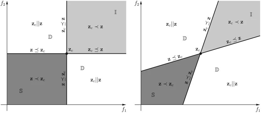
Fig. 1. Left: Dominance relations defined by a coneK=Rk
+, in this instance K=R 2
+. Right: Dominance relations defined by an acute proper cone
K={z:Pk
i=1θizi, θi≥0}withziforming an acute angle withzjfor alli6=j. The region,Scontains superior solutions tozcand the regionIinferior solutions, whileDis the union of all the regions in,Z, that contain incomparable solutions tozc. A mnemonic for the notation of the regions in the above
figures is Superior forS, Inferior forIand non-Dominated for theDregions respectively.
ordering induced by the binary relations≺,is called partial because of the following possibility: x,y ∈ Z but x y
and y x, in which case the vectors x,y are said to be
incomparable. For example, the vectors x = (3,2,1) and
y= (1,2,3) are incomparable. Dominance relations induced by two different proper cones are depicted in Fig. (1). Pareto-dominance relations and Pareto-dominance relations imposed by the setK=Rn
+\0are equivalent [1, pp. 24]. Notice that the0
element is removed fromK, this means that Pareto-dominance relations are not reflexive, i.e. x K x does not hold as,
x−x=0∈/ K.
Most multi-objective problem solvers attempt to identify a set of Pareto optimal solutions, this set is a subset of the Pareto
optimal set (PS) which is also referred to as Pareto front
(PF). The Pareto optimal set is defined as follows: P ={z: ∄˜z z,∀˜z ∈Z}, namely, it is the set of objective vectors that are not dominated by any objective vector in the feasible objective space. The decision vectors whose forward image under the objective function is the set,P, are also referred to as the Pareto set and are denoted as D, namelyF:D → P. That is, the decision space is implicitly ordered according to the partial ordering applied to the objective space.
Algorithms based on Pareto dominance based methods for tackling multi-objective (and many-objective) problems have several difficulties to overcome. For instance a well distributed Pareto front is not guaranteed simply by using dominance relations. One answer to this problem has been presented in [48], where the authors introduce ε-dominance. In essence, ε-dominance creates a strict partial ordering based on the set Kε = Rk+ + ε. This type of dominance relation is
useful to maintain well distributed Pareto optimal solutions [48], however it cannot escape the deficiency that Pareto-based methods face in many-objective problems [27]. Another very interesting approach introduced in [49], termed cone ε -dominance, uses the union of an acute proper cone and the setKε=Rk++εto define a relation that is a partial ordering.
Namely, they use ε-dominance in combination with an acute
cone,Kα={z:Pki=1θizi, θi≥0}withzi forming an acute
angle with zj for all i 6=j. Therefore, cone ε-dominance is
defined with the help of the set Kc =Kε∪Kα. The partial
ordering induced by an acute cone is shown in Fig. (1). The motivation for the introduction of this type of Pareto domi-nance is that the diversity of produced Pareto optimal solutions seems to be better. Namely, cone ε-dominance promotes a good spread of solutions across the entire Pareto front, and, their distribution seems to be more uniform. However, the problem reported in [27] persists for this type of dominance as well. In fact, since the regions where solutions become non-comparable are larger in coneε-dominance it is expected that the number of non-dominated solutions increase more rapidly, compared to the Pareto dominance using K = Rk
+,
see Fig. (1).
B. Bias in the Objective Function
In the following sections of this work we assume that the objective function is unbiased or that it is not biased towards the Pareto front. This term is related to what the authors of the WFG10 toolkit [50] refer to as bias in the objective function. An objective function is considered to be unbiased when for decision vectors that are uniformly distributed inS the resulting distribution in objective space is also uniform, or close to uniform [50]. In this work we employ the same notion of bias, however we also provide a definition which should clarify the underlying assumptions of the statements: “an objective function has no bias”, or “an objective function is biased toward the Pareto front” etc. Specifically, let X be an independent random deviate distributed according to,U(S), namely a uniform distribution in the feasible decision space, then we say that the objective function,F, has no bias if,
F(U(S)) =Z ∼ U(Z). (6)
10Walking Fish Group. The WFG toolkit can be used to create scalable test
In other words, a uniformly sampled decision space maps to a uniformly sampled objective space, or at least approximately so. In some fortunate cases, the objective function is biased towards the Pareto front, namely,
Z . . .
| {z } k
Z
B
h(z1, . . . , zk)dz1. . . dzk >PU(Z ∈B),
B={z: inf{kz−zpk} ≤r,zp∈ P,z∈Z},
(7)
where h, is the probability density function (pdf) of the objective space and B is the set of all feasible objective vectors with distance r or less from the Pareto front. So if the probability (the integral in (7)) to obtain a solution in B is larger for,h, than the uniform distribution then we say that the objective function is biased towards the Pareto front. If (7) holds forBc, the complement ofB, then we say that the
objective function is biased away from the Pareto front. Similar definitions for bias toward any other region in objective space are trivial to define by simply changing the definition of the setB.
C. Pareto Dominance for Many-Objective Problems
In [27] the authors provide empirical results in an attempt to explain the reason for the poor performance of Pareto dominance-based algorithms applied to many-objective prob-lems. The main argument is that the ratio of non-dominated (incomparable) individuals to the size of the population is approaching 1, meaning that almost the entire population is non-dominated, therefore the algorithms’ selection mechanism is provided with no useful information. In what follows we elaborate further on this argument and prove that this be-haviour is to be expected in many-objective problems and we reveal, to an extent, the underlying cause for such difficulties. Consider the simplest multi-objective case, namely a 2 -objective problem. Every point in -objective space defines 4
regions shown in Fig. (1), (i) a region that contains solutions that are clearly better denoted asS, (ii) a region that contains solutions that are clearly worse, I, and (iii, iv) two regions where the solutions are incomparable to the point in question,
D. For 3-objective problems there are 8 such regions (23
), however there is only 1 region which contains clearly better solutions and1 region with clearly worse solutions. So, there are 23−2 = 6 regions that contain solutions incomparable
to the point in question. In general the following is true, for k-dimensional problems, there is always1 region with clearly better solutions, 1 region with clearly worse solutions and
2k−2regions containing incomparable solutions. Furthermore,
assuming that there is no bias towards any of these regions in the problem (objective function), the probability that a solution is generated in any one of these regions by a stochastic process (algorithm) is proportional to the volume of these regions divided by the volume of the entire feasible set in objective space11,Z. However, for increasing number of dimensions, the likelihood that a solution will be generated within the region
S, becomes almost insignificant the closer the point is to the
11We assume that the feasible objective set is bounded.
Pareto front. For example, for 10dimensions there are1 024
regions, hence for the above problem, the probability for a solution to be generated, that dominates the current point, is approximatelyp= 1/1 024 = 9.76−4 if the point in question
is exactly in the middle of a feasible objective space. To contrast this, the probability that a non-comparable solution is generated is 1 022/1 024≈0.99.
Although the assumption that the problem has no bias seems to limit the generality of the above argument, this is not entirely true. To illustrate this let us consider the relative
directions of bias in the objective function in the context of
optimization. These bias can be: (i) towards the Pareto front, namely it is easier to obtain solutions near the PF than in any other region, (ii) towards the region containing clearly worse solutions, and (iii) towards any region or regions con-taining incomparable solutions. Only in case (i) the solution of the optimisation problem becomes easier compared with the unbiased version. However this favourable scenario is seldom encountered in practice. So by assuming no bias in the objective function, all the probabilities that we calculate are in the worst case upper bounds on the probabilities of obtaining solutions in the setS. In other words, the probabilities reported in this work represent the best attainable probability with respect to the location of an objective vector. We elaborate further on this point in Section VI.
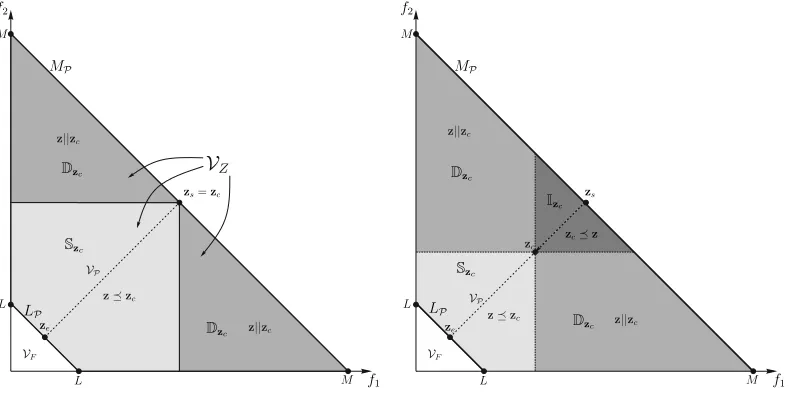
To better appreciate and understand the reasons for the apparent difficulties that many-objective optimization algo-rithms face with such problems, we frame the aforementioned example on a more concrete basis. Assume that the objective space, Z, is bounded from above by a hyperplane as shown in Fig. (2), specifically the upper bound is the set of points MP ={z:
Pk
i=1zi =M, zi≥0}. The reasons for selecting
a feasible objective region with this particular geometry will become clear in what follows. Also, let the Pareto front be a (k−1)-simplex, namely Pareto optimal objective vectors are part of the set LP = {z : Pki=1zi = L, zi ≥ 0},
obviously we have to selectL < Mfor minimization problems as L > M would imply Z={∅}. If we also assume that the problem has no bias, then given an objective vector,zc ∈Z,
it would be possible to calculate the probability of obtaining a better solution for any point in the objective space. This information can be useful in many ways, we elaborate on those in Section VI.
Now, given a point in objective space,zcwhere the subscript
is an abbreviation for current point, we can calculate the probability of obtaining a better solution using the following relation,
P(z∈S|zc) =
VS(zc)
VZ
, (8)
where,VS(zc) =VP(zc), for Pareto-based methods,VZ is the
volume of the feasible objective space which is equal to the
volume of the slab in betweenMP,LPand the positive orthant
Rk
+, see Fig. (2). Additionally,P(z∈S|zc), is the probability
of finding a better objective vector, zn, given the objective
vector zc. The expression in (8) is valid only for problems
Fig. 2. Trajectory for the experiment described in Section III-D comparing decomposition and Pareto-based methods.MPis the upper bound of the feasible
objective space whileLPis the Pareto front and the lower bound of the feasible objective space. AlsoVF is the volume below the Pareto front andVZ is the volume of the feasible objective space, whileVPis the volume of the region containing superior solutions to the current solutionzc. Lastly,zs andze are the starting and target objective vectors, withzebeing Pareto optimal. The left figure illustrates the aforementioned quantities forzc=zsand the right
figure illustrates how the above quantities change aszcmoves towardsze along the(ze−zs)direction. The results can be seen in Fig. (3).
the exact probability density function in objective space would be necessary so that we can weigh the integrals. However, as we mentioned above, in all but the most trivial problems the bias will be towards the Pareto front, otherwise it will be away from it, and so (8) will still describe a useful quantity, namely the upper bound of the probability of finding a better solution, assuming that there is no bias towards the Pareto front.
The volume of the region containing clearly better solutions,
VP(zc), for Pareto dominance or cone dominance using an
ordering cone K=Rk + is,
VP(z) =
k Y
i=1
zi− VF, (9)
whereVF is the volume of the non-dominated region beneath
the Pareto front, which is the volume beneath the simplex,LP.
The (k−1)-simplex corresponds to a Pareto front with affine geometry and VF is calculated as,
VL=
det v1 · · · vk
Γ(k+ 1) . (10)
Here,vi, are the vertices that the Pareto front intersects with
the axes. The vectors, vi for the Pareto front are equal to
vi =L·ei, whereei is a vector of zeros and itsithelement is
equal to one. Furthermore, the volume beneath the hyperplane MP,VM, is calculated using (10) andvi=M·ei. OnceVM
andVLhave been evaluated, the volume of the entire feasible
objective space is calculated as,
VZ =VM− VL. (11)
Also the volume of the non-dominated region forε-dominance is simply,
VPε(z) =
k Y
i=1
(zi−ε)− VF, (12)
assuming that the sameεvalue is used for every objective. If different values forεare used it is trivial to modify (12). The volume of the non-dominated region for cone ε-dominance [49] is much more involved to calculate exactly, however, given that its defining set is the intersection of a proper cone and the set Rk+ε it stands to reason that its volume,VKε,
will be within,
VPε ≤ VKε ≤ VP, (13)
depending on the selected acute cone.
D. Experiment
Using (8)-(10) and a trajectory in objective space we can explore the change in the probability to obtain a solution in S from a current point, zc. So, assume we start from
a point that is on the upper bound of the objective space,
zs ∈ MP, and a target point on the Pareto front ze, the
question is how likely is to find a better solution with respect to any point on the trajectory with direction ze −zs, see
Fig. (2). The trajectory that the pointzc follows can be seen
in Fig. (2) is simply the line segment between zs and ze.
This information for Pareto dominance methods will give us a basis for comparison with other methods for inducing a partial order in the objective space and should illuminate any differences. The steps involved, for this and for decomposition-based methods described in Section IV, as follows:
• Set zc = zs. Subsequently we divide the line segment
from zs to ze into N−1 segments, thus from start to
end there are N points zc[i] = zs+ (ze−zs)Ni and i= 0, . . . , N−1, see Fig. (2).
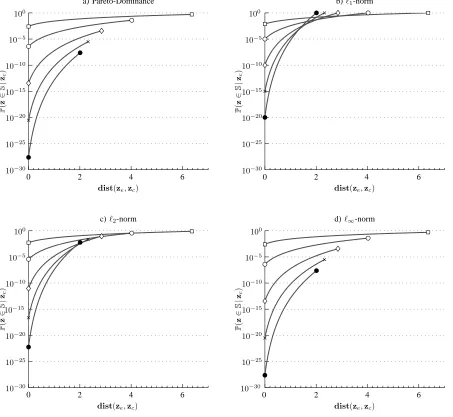
• For every zc[i] we calculate (8). The results are shown
dist(ze,zc)
P
(
z
∈
S
|
zc
)
a) Pareto-Dominance
dist(ze,zc)
P
(
z
∈
S
|
zc
)
b)ℓ1-norm
dist(ze,zc)
P
(
z
∈
S
|
zc
)
c)ℓ2-norm
dist(ze,zc)
P
(
z
∈
S
|
zc
)
d)ℓ∞-norm
0 2 4 6
0 2 4 6
0 2 4 6
0 2 4 6
10−30
10−25
10−20
10−15
10−10
10−5
100
10−30
10−25
10−20
10−15
10−10
10−5
100
10−30
10−25
10−20
10−15
10−10
10−5
100
10−30
10−25
10−20
10−15
10−10
10−5
[image:9.612.85.538.59.476.2]100
Fig. 3. Probability to find a better solution tozc,P(z∈S|zc), as a function of the Euclidean distance of the solutionzctoze, denoted bydist(ze,zc),
for different number of objectives (see Fig. (2)). Here{,◦,⋄,×,•}correspond tok={2,5,10,15,20}objectives respectively.
IV. DECOMPOSITIONMETHODS
A. Overview
An alternative for defining a partial order in objective space, and of course an implicit partial order in decision space, can be found in decomposition methods. As mentioned in Section I, these methods employ a scalarizing function to aggregate all the objectives into a single scalar objective function. To obtain different Pareto optimal points, a set of weighting vectors can be used which would result in a set of single objective
subproblems. This is the reason why such methods are called decomposition-based, it is because the employed strategy is
to decompose a complex problem into a set of simpler ones. Simpler in this context does not necessarily mean easier to solve, it means that it is straightforward to apply standard EAs to the resulting subproblems.
The family of scalarizing functions that we focus our attention in this work, is the weighted metrics method [1, pp.
97] defined as:
min
x k X
i=1
wi|fi(x)−zi⋆|p !p1
, (14)
where, wi are the weighting coefficients, wi ≥0 for all i= 1, . . . , k, andPki=1wi = 1, alsop∈(0,∞). The vectorz⋆= (z1, . . . , zk), is called the ideal vector and is defined asz⋆= (inf
x {f1(x)}, . . . ,infx {fk(x)}). For the purpose of this work we will assume that z⋆ = (0, . . . ,0), which means that (14)
can be rewritten as,
min
x k X
i=1
wifi(x)p !1
p
. (15)
Notice that we are allowed to remove the absolute value while maintaining the equivalency relation between (14) and (15), since,z⋆ = (0, . . . ,0), implies thatz∈Rk
+. The formulation
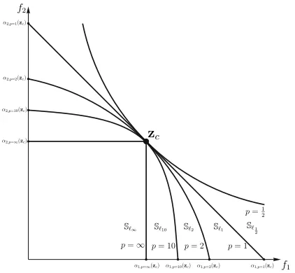
Fig. 4. The curves in the left figure represent the boundary of solutions that will be perceived as clearly better with respect to the correspondingp-norm. A geometric (although not entirely true) explanation as to why the Chebyshev scalarising function (p = ∞) guarantees the generation of Pareto optimal solutions is seen to the right. In effect Chebyshev scalarising function creates something that resembles a asymptotically stable equilibrium. This seems to be the case for anyp-norm withp >1.
Chebyshev decomposition. Namely, for p= 1 we obtain the weighting method [1, pp. 78],
min
x k X
i=1
wifi(x), (16)
while for p = ∞ we obtain the Chebyshev scalarizing function,
minx (max{w1f1(x), . . . , wkfk(x)}). (17)
A derivation of (17) from (15), is included in Appendix A for completeness. It should be noted that the assumption that the ideal vector is equal to the zero vector also implies that the objective function is bounded from below. In extension if the ideal vector is known and is not zero a change of variables in the objective function would be sufficient to meet our assump-tion. For example, for z⋆= (−2,4), it suffices to change the
objective function, F, withF˜(x) = (f1(x) + 2, f2(x)−4).
Although all norms are equivalent, in the sense that for every norm in a finite dimensional space multiplicative con-stants can be found relating two norms [2, pp. 636], their effect in an optimization problem can be significantly different, depending on the intricacies of the problem. For example, for p = ∞, namely the Chebyshev scalarizing function, there exist theoretical results stating that the solutions of (17) will be at least weakly Pareto optimal for any weighting vector
w ∈ Rk
+ and that any Pareto optimal solution can obtained
for some weighting vector [1, pp. 99]. The interest of the MOEA community with respect to this particular norm is that the previous statement holds for nonconvex problems as well. Note that this does not imply that there is a guarantee that the algorithm will be able to find a Pareto optimal solution for a nonconvex problem, rather the statement refers to the equivalency of the two problems. In other words, assuming
that the selected algorithm is able to solve the problem defined in (17) then the solution will be at least a weakly Pareto optimal, and that all the Pareto optimal solutions can be obtained for some weighting vector. Such a result does not exist forp <∞. In Section V we show that, given some prior information, it is possible to find a norm other than infinity with the same properties mentioned above. Namely, the ability of the a scalarized problem to converge to a weakly Pareto optimal solution for every weighting vector w ≻0 and that all Pareto optimal solutions can be reached.
However, it is not obvious as to why a norm, other than the ℓ∞-norm that is employed in the Chebyshev scalarizing
function, would be more useful for decomposing a many-objective problem. For this reason we extend the experiment conducted for Pareto-based methods to decomposition-based methods that employ (15) as the scalarizing function to de-compose a many-objective problem and study the effects that different values of phave on the resulting subproblems, see Section IV-B.
B. Decomposition Methods for Many-Objective Problems
The difference between scalarizing functions and the various forms of dominance relations discussed in Section III, is that the former define a complete ordering in the objective space, namely for a subproblem defined as,
gp(x) = k X
i=1
wi|fi(x)−zi⋆|p !1
p
, (18)
then for any two decision vectorsx,˜x∈Z, only one of the following relations obtains,
gp(˜x)< gp(x), orgp(˜x) =gp(x), orgp(˜x)> gp(x),
given that the two decision vectors are applied to the same subproblem. Namely, regions containing incomparable solu-tions (regionsDin Fig. (1)) are eliminated, and depending on theℓp-norm used in (15), parts of theDregions are absorbed
by the region containing inferior solutions, I, and the region containing clearly better solutions, S. This phenomenon has the potential to reduce the rate of decrease of the probability that a better solution is generated as the current solution approaches the optimal point, see Fig. (3)-(b-d). A better solution in this context is a solution that yields a lower value for the selected scalarizing function. In turn, this can reduce algorithm stagnation due to large number of non-dominated solutions as is the case in Pareto-based methods [27]. To see this consider a scenario in which the weighted sum method is used. In this scenario the weighting vector represents the normal of a hyperplane that divides the feasible objective space in two partitions. One, a region containing better solutions,
Sℓ1, and one with worse solutions, Iℓ1, shown in Fig. (4).
the currently best objective vector. However we have made a concession here, as the new solution may not Pareto-dominate the previous best solution. We will return to this issue in Section V and Section VI.
To explore how decomposition-based methods relate to Pareto-based methods, we must be able to calculate (8) for everyp= (0,∞]. The volume of the feasible objective space is calculated in the same way as in (11), while the volume of the S region forp= (0,∞)is calculated as:
VS ℓp(z) =
Γ1 +1 p
k
Γk p+ 1
· k Y
i=1
αi(z)− VF, (19)
which is essentially the volume of the positive orthant of a hyperellipsoid calculated as seen in [51]. The factors ai(z)
represent the distance of the ideal vector from the intersection of the ellipsoid with the positive axis of the ith objective,
shown in Fig. (4) and are calculated as,
αi(z) = Pk
m=1wmzpm wi
!1
p
, (20)
see [51]. Since for the special case thatp=∞,
lim p→∞
Γ1 +1 p
k
Γk p+ 1
= 1, (21)
the volume of the Sregion becomes,
VSℓ∞(z) =α1(z). . . αk(z)− VF, (22)
and,
αi(z) =
max{w1z1, . . . , wkzk} wi
. (23)
Furthermore, to replicate the selected trajectory described in Section III-C and shown in Fig. (2), the weighting vector is set to w = 1
k ·(1, . . . ,1) ascribing equal importance to all
objectives so the resulting subproblem will tend to follow this trajectory and converge to the point ze. For this particular
weighting vector (22) becomes,
max{w1z1, . . . , wkzk}=wmzm,
VSℓ∞(z) =
(1 k)
kzk m (1
k)k
− VF =zkm− VF.
(24)
However, as can be seen in Fig. (2), all points in the trajectory from zs to ze have z1 =z2 =· · · =zk, hencezm =zi for
all i= 1, . . . , k, thus (24) can be calculated for any point on the trajectory.
As seen in Fig. (3)-(a-d), the probability to find a better solution as zc approaches the optimal solution ze decreases
more rapidly for the Chebyshev scalarizing function and Pareto-based methods when compared to scalarizing functions employing the ℓ1-, ℓ2-norm. However, the results for the
Chebyshev scalarizing function are remarkably similar to the Pareto-based method. In fact, for this trajectory, the two are identical, see (9) and (24). This interesting result means that Pareto-based methods and decomposition-based methods using
the Chebyshev scalarizing function are identical in the sense that,
VSℓ∞ =VP. (25)
This result is quite intriguing given the increased number of reports showing decomposition-based algorithms outper-forming their Pareto-based counterparts for many-objective problems (cite some). However, we have only shown that the above equality holds for one particular trajectory and not necessarily for every possible trajectory towards any point on the Pareto front. We claim that (25) holds for an entire family of trajectories and that these particular trajectories are the ones that both decomposition and dominance-based algorithms attempt to follow in their approach towards the PF.
Before the general case is examined, consider a subproblem defined by the following weighting vector,
wi= 2i k(k+ 1),
w=
2
k(k+ 1), . . . , 2k k(k+ 1)
(26)
furthermore the selected starting pointzs, is,
zs=M·
k(k+ 1) 2 , . . . ,
k(k+ 1) 2k
(27) and the end solution, ze, that is the target Pareto optimal
solution is,
ze=L·
k(k+ 1)
2 , . . . ,
k(k+ 1) 2k
. (28) Therefore any solution on the trajectory will be,
C∈[L, M],
zc=C·
k(k+ 1)
2 , . . . ,
k(k+ 1) 2k
. (29) Given (26)-(29),
VP(zc) = k Y
i=1
zi− VF =
(Ck(k+ 1))k
2kk! − VF. (30)
To calculate the volume of S for the Chebyshev scalarizing function we need to find what is the maximum element. However, a closer look at (26) and (29) will reveal that this element is simply C, hence,
VSℓ∞(zc) = k Y
i=1
αi− VF =
(Ck(k+ 1))k
2kk! − VF, (31)
so the relation VSℓ∞(zc) = VP(zc) holds for this weighting
vector as well. At this point we need to justify the assumption that a solution will attempt to follow the trajectory defined by the weighting vector in (26), since it appears to be artificial. For this we refer to the work by Ballestero [52] where he refers to this trajectory as well-balanced baskets due to the relation,
w1z1=w2z2=· · ·=wkzk, (32)
most easily observed in the ℓ∞-norm used by the Chebyshev
decomposition whereby only the largest deviation is taken into account thus reeling the solution toward the balanced trajec-tory. For example given an objective vector z = (1,1.1,1)
and a weighting vector12 w = (0.33,0.33,0.33), the ℓ
∞
-norm will attempt to minimize the second component of, z, simply becausemax{0.33·1,0.33·1.1,0.33·1}= 0.3667. By this reasoning, when the ℓ∞-norm is used in a minimization
problem, the focus of the algorithm will be to maintain the Hadamard productw◦zas close as possible to the vectorM·1
while attempting to reduceM. By changing the weighting vec-tor, this equilibrium that the Chebyshev scalarizing function is attempting to maintain, changes, so a different trajectory is followed, which of course converges to a different Pareto optimal point if the optimization algorithm is successful. Well that trajectory is found by finding the objective vector that
sends the weighting vector w to the unit vector. Therefore for any given weighting vector,
w=c1
s, . . . , ck
s
,
s= k X
i=1
ci,
(33)
the balanced trajectory for theℓp-norm withp= (0,∞)is the
set of points given by,
zc=C· s c1
1
p
, . . . ,
s ck
1
p!
,
s= k X
i=1
ci, ci∈R+,
(34)
and for theℓ∞-norm by,
zc =C·
s c1
, . . . , s ck
,
s= k X
i=1
ci, ci∈R+,
(35)
and therefore since,
VSℓ∞(zc) =
(max{w1zc,1, . . . , wkzc,k})k Qk
i=1wi
− VF
= C
k
Qk i=1ci
sk
− VF = (Cs)k Qk
i=1ci
− VF
(36)
and,
VP(zc) = Y
i=1
kzc,i− VF = (Cs)k Qk
i=1ci
− VF, (37)
meaning that VP(zc) = VSℓ∞(zc) whenever the objective
vectors are allowed to follow the balanced trajectory that the Chebyshev scalarizing function attempts to follow. Notice that this results also hold for for biased objective functions.
12An over-line a number denotes infinite repetition of the digits below, e.g.
0.33 = 0.33....
It follows that for objective vectors following a balanced trajectory,
VSℓ
1 >VSℓ2 >· · ·>VSℓ∞ =VP. (38)
A proof for (38) is given in Appendix A-A. Meaning that,
Pℓ1(z∈Sℓ1|zc)>Pℓ2(z∈Sℓ2|zc)> . . .
>Pℓ∞(z∈Sℓ∞|zc) =PP(z∈S|zc),
(39) wherez∈Z andSℓpis the region containing better solutions
according to the ℓp-norm version of the scalarizing function
andPℓp(z∈Sℓp)is the probability of finding a better solution
inSℓp given that the current best solution is zc. The result in
(39) can be read directly from Fig. (4).
V. SCALARIZATION ANDSTABILITY OF THEEQUIVALENT
PROBLEM
The results in the previous section must be interpreted with care since (39) does not imply in any way that by using a scalarizing function based on a norm with p < ∞, all the Pareto optimal solutions will be reachable. However it does imply that by using a scalarizing function withpsmall, there is a better chance in finding better solutions with respect to that norm. Nevertheless, we require Pareto optimal solutions and not just any solutions that are closer to the front in someℓp
-norm, which means that if we cannot ensure that the subprob-lems are able to converge to Pareto optimal solutions and that all Pareto optimal solutions will be obtainable, the importance of (39) would be limited to the fact that Pareto-dominance methods are equivalent to decomposition-based methods that employ the Chebyshev scalarizing function. Equivalent in the sense that for an objective vector following a well balanced trajectory the probability to obtain a solution dominating the current solution is the same in both methods.
To understand the tradeoff between using a dominance-based method versus a decomposition-dominance-based method let us consider the effect of a scalarizing function to the objective space. A scalarizing function projects the entire objective space onto a line13, therefore some regions that contain
incom-parable solutions in the Pareto sense, now become solutions that are either better or worse for the particular subprob-lem. Therefore, a major difference between decomposition-based and Pareto-decomposition-based algorithms is that the former provide unambiguous information about the quality of the produced solutions at every iteration while the latter cannot always guarantee such information because the likelihood of gen-erating incomparable solutions is high for problems with many objectives [27]. However it is easy to reduce the above argument into a zugzwang14 between Pareto-based methods
and decomposition-based methods. This is accomplished by the simple observation that the clearly better regions in the Chebyshev scalarizing function (p = ∞ in Fig. (4)) are
13In this work a segment of a ray, since the objective space is bounded. 14A chess terminology whereby the player whose turn is to play will be at a
Fig. 5. Stable and unstable scalarizing functions.
identical to the regions generated by Pareto dominance based methods (Fig. (1)), while the incomparable and clearly worse regions in Pareto-based methods are mapped to clearly worse regions by the Chebyshev scalarizing function. Namely, if we require a decomposition method that can guarantee the generation of Pareto optimal solutions, then, we have to use the Chebyshev scalarizing function but in so doing we give up the favourable convergence rates15 achieved when using, for example the weighted sum method, and vice versa. In general there are two competing trends:
• Asp→0, the probability of finding a better solution with
respect to the ℓp-norm increases, hence it is less likely
that the algorithm stagnates due to its inability to find direction of search. Additionally, it becomes increasingly more difficult to obtain all Pareto optimal solutions.
• However, asp→ ∞, we can obtain more Pareto optimal
solutions on the Pareto front, but the probability to find a better solution with respect to the norm defined byp is also decreasing. In the limit, namely forp =∞, we obtain the Chebyshev scalarizing function that guarantees that we will be able to find all Pareto optimal solutions for some weighting vectorwbut this scalarizing function is equivalent with Pareto-dominance methods.
So the question is: is there a way that a scalarizing function can be used with p relatively small while preserving the guarantees that the Chebyshev function provides? The answer is affirmative for many-objective problems whose Pareto front geometry is continuous (see Section II). Specifically, a Pareto front can be described with the following parametrization,
fp1 1 +f
p2
2 +· · ·+f pk
k =C, (40)
where pi > 0 for all i and C is a positive constant.
For simplicity we assume that fi ≥ 0. We claim that if
the weighted metrics scalarizing function is used with p = max{p1, . . . , pk}, then this scalarization will have the same
guarantees as the Chebyshev function, given that our estimate ofmax{p1, . . . , pk}is correct and that the objective function is
15Or more correctly the potential for favourable convergence rates.
continuous. The reason for this is illustrated in Fig. (5). To see this, consider that whenzc reachesze in Fig. (5), the volume
of the regionSℓ1is still positive, meaning that according to the
ℓ1-norm there are still better solutions to the current solution.
Continuing on the same line of reasoning, the solutionzcwill
either converge tozAorzB since at these two locations there
is no way that theℓ1-norm to be improved. This result follows
directly from (38) and the results in [51] for calculating the volume in (40), it follows that,
lim
zc→ze VPz− Vℓp
≤0, (41)
when p > max{pi}. In which case we say that the
scalar-ization is stable while if p < max{pi} the scalarization is
unstable and we have,
lim
zc→ze Vℓp− VPz
>0. (42) Stability in terms of sclarizations is taken to mean the follow-ing:
• A subproblem of a many-objective problem is a stable
scalarization if for a given weighting vector w ≻0, it is able to converge to a Pareto optimal solution ze = (z1, . . . , zk), withzi >0 for everyi= 1, . . . , k.
• Conversely, a subproblem is an unstable scalarization
if for a given weighting vectorw≻0, it converges to a Pareto optimal solution ze with zi = 0 for at least one i∈ {1, . . . , k}.
Therefore if the Pareto front geometry is known and it can be expressed in terms of (40), then we can select the ℓp-norm that will have the maximum probability to produce
better solutions while preserving the guarantee that the final population will be (weakly) Pareto optimal and that all the Pareto optimal solutions will be obtainable for some weighting vector.
VI. DISCUSSION
problem. Namely, the question that can now be posed is: “what is the optimal ℓp-norm for the scalarization and trajectory
for an objective vector?”. By optimal trajectory we mean the trajectory in objective space that will present the least
resistance to our optimization algorithm while simultaneously
moving towards a Pareto optimal solutions as fast as possible. This question although very interesting, it has either a trivial answer: a straight line, or for biased problems we would need to have knowledge of the probability density function in objective space, something which in general is unavailable even for test problems. Therefore, we use a balanced trajectory, since this is in accord with the scalarizing functions, in the sense that this is the path that they tend to follow. Using this we investigated how the probability to obtain better solutions varies as a function of the distance of the current best solution and the sought for Pareto optimal solution. We found that this probability is largest the smaller the ℓp-norm is, with respect
top. This information can be used to reduce the difficulty of many-objective problems, to some extent.
However, we cannot simply use the smallest norm that is numerically feasible since with decreasing pthe ability of a scalarizing function to converge to a particular point of the Pareto front is also reduced, hence, a concession must be made. Although, if the Pareto front is continuous and can be described in a parametric way (see (40)), an optimal value, p⋆, can be obtained for which the decrease of the probability
of finding a better solution is minimal while the ability of the scalarizing function of finding every Pareto optimal solution is retained. The optimal value of p, separates the family of scalarizing functions into two subclasses. First, values of p < p⋆ produce unstable scalarizing functions and p > p⋆
result in stable scalarizing functions. Here stability refers to the ability of the scalarizing function to converge to any point on the Pareto front, while instability refers to the opposite.
A way to convexify the Pareto front, and thus allowing for an arbitrarily small16 ℓ
p-norm to be used, has been proposed
in [53]. Essentially, what the author of the aforementioned work suggested is that the objective function is raised to a power until the Pareto front becomes convex. Although this suggestion may seem intriguing, the effect of such a non-linear operation to the objective function would be, among other things, introducing bias in the objective function and potentially making the problem more difficult to solve in the case that the initial set of scalar objective functions are non-convex.
VII. CONCLUSION
Based on the results in Section III and Section IV we have seen that under mild conditions the Chebyshev function is identical to Pareto-dominance methods. Identical in the sense that, for a solution following a balanced trajectory, the reduction of probability to find a better solution is iden-tical for both methods. This curious fact suggests that the decomposition-based methods are actually not better com-pared with Pareto-based methods. But if that is so, how can the results observed by several researchers for many-objective
16Small here refers top.
problems be justified? Given the fact that the reported results are only slightly better in [30]–[33] our hypothesis is that the difference is simply due to the ease with which a constant direction of search in objective space can be maintained in decomposition-based methods, while the same is very difficult to achieve with Pareto-based methods. A good example of this behaviour is seen in MOGLS17 [54] when compared
with MOEA/D in [34]. In the aforementioned work MOGLS was outperformed by MOEA/D, and as the authors note, one reason was that MOGLS generated different weighting vectors on every iteration. This amounts to an attempt to identify the entire Pareto front, but also means that the direction of search in objective space is not constant as is the case for MOEA/D. The same problem is present in Pareto-based methods, however there is no clear way for this situation to be remedied.
The results in this work show that:
• Pareto-dominance methods and the Chebyshev
scalar-izing function are equivalent, in the sense that neither method in itself, has better probability to find superior solutions. In fact the aforementioned probabilities are the same.
• Given some prior information about the problem, namely
the geometry of the Pareto front, we can find the optimal scalarizing function. Optimal in this context means that using the above scalarizing function all Pareto optimal so-lutions will be obtainable for some weighting vector, and that, the probability of obtaining a better solution, with respect to the particular scalarizing function, decreases more slowly compared to all other scalarizing functions (and Pareto-dominance methods) that can provide the same guarantee of finding all Pareto optimal solutions.
• Using generalized decomposition (gD) [55], [56] in
conjunction with the results in this work, the required weighting vectors for obtaining Pareto optimal solutions in specific locations on the Pareto front, can be identified for anyℓp-norm.
Some of the mentioned benefits apply only when we are able to identify the Pareto front geometry prior to obtaining Pareto optimal solutions. We have identified a solution to this problem and preliminary results seem very promising.
APPENDIXA
GAMMAFUNCTIONDEFINITION ANDNORMVOLUMES
TheΓ function18 is defined as:
Γ(x) = Z ∞
0
tx−1
e−xdt. (43)
Forx∈N,
Γ(x+ 1) =x!. (44)
The psi or digamma function is [57], ψ(x) = d
dx((ln (Γ(x)))
=−γ−1
x+
∞
X
n=1
1
n−
1
x+n
.
(45)