City, University of London Institutional Repository
Citation
:
Karouzakis, N., Hatgioannides, J. & Andriosopoulos, C. (2017). Convexity
Adjustment for Constant maturity Swaps in a Multi-Curve Framework. Annals of Operations
Research, doi: 10.1007/s10479-017-2430-6
This is the published version of the paper.
This version of the publication may differ from the final published
version.
Permanent repository link: http://openaccess.city.ac.uk/17896/
Link to published version
:
http://dx.doi.org/10.1007/s10479-017-2430-6
Copyright and reuse:
City Research Online aims to make research
outputs of City, University of London available to a wider audience.
Copyright and Moral Rights remain with the author(s) and/or copyright
holders. URLs from City Research Online may be freely distributed and
linked to.
City Research Online: http://openaccess.city.ac.uk/ [email protected]
DOI 10.1007/s10479-017-2430-6
A NA LY T I C A L M O D E L S F O R F I NA N C I A L M O D E L I N G A N D R I S K M A NAG E M E N T
Convexity adjustment for constant maturity swaps
in a multi-curve framework
Nikolaos Karouzakis1 · John Hatgioannides2 ·
Kostas Andriosopoulos3
© The Author(s) 2017. This article is published with open access at Springerlink.com
Abstract In this paper we propose a double curving setup with distinct forward and dis-count curves to price constant maturity swaps (CMS). Using separate curves for disdis-counting and forwarding, we develop a new convexity adjustment, by departing from the restrictive assumption of a flat term structure, and expand our setting to incorporate the more realistic and even challenging case of term structure tilts. We calibrate CMS spreads to market data and numerically compare our adjustments against the Black and SABR (stochastic alpha beta rho) CMS adjustments widely used in the market. Our analysis suggests that the proposed convexity adjustment is significantly larger compared to the Black and SABR adjustments and offers a consistent and robust valuation of CMS spreads across different market conditions.
Keywords Convexity adjustment·Constant maturity swaps·Multi-curve framework· Yield curve modelling·Money market instruments
1 Introduction
The recent financial crisis has led, among others, to unprecedented behavior in the money markets, which has created important discrepancies on the valuation of interest rate financial instruments. Important reference rates that used to be highly correlated and moving together for a long period of time, started to diverge from one another. A characteristic example,
B
Nikolaos KarouzakisJohn Hatgioannides [email protected]
Kostas Andriosopoulos [email protected]
1 School of Business, Management and Economics, University of Sussex, Brighton BN1 9SL, UK
2 Cass Business School, City University London, 106 Bunhill Row, London EC1Y 8TZ, UK
that has been widely studied recently, is the widening of the spread between deposit rates (Libor/Euribor) and overnight index swap (OIS) rates of the same maturity. At the same time, the market started observing non-zero spreads between swap rates of the same maturity, but based on different frequencies of the underlying Libor rate, or between forward rate agreement (FRA) rates and forward rates implied by consecutive deposits. These examples indicate that financial players consider each tenor as a separate market, incorporating different credit and liquidity premia, and as such, each one of them is driven by its own dynamics.
Such discrepancies have, above all, questioned the methodology used to bootstrap the yield curve, which has created a layer of uncertainty on the methods used to price and hedge interest rate financial instruments. There are three main issues associated with the pre-crisis approach, which make it inconsistent. First, the information incorporated into the basis spreads is not taken into account. Second, using a single yield curve does not allow us to consider the different dynamics introduced by each underlying rate tenor, making hedging and pricing of interest rate derivatives less stable. Finally, the no-arbitrage assumption indicates that a unique discounting curve needs to be used, regardless of the number of the underlying tenors. In order for market participants to comply with the mentioned market features, they started building a separate forward curve for each given tenor, so that future cash flows are generated using the appropriate curve associated with the underlying rate tenor. At the same time, a single and unique discounting curve had to be used, in order to calculate the present value of contract’s future payments. This led financial players to start using the OIS swap curve, rather than the Libor curve, for the construction of a riskless term structure. The reason behind their choice was mainly twofold. First, OIS is believed to contain very little credit and liquidity risk premia compared to Libor rates. Second, the fact that most trades in the interest rate market are (mainly cash) collateralized makes the funding cost for a financial institution no longer equal to the Libor rate, but to the collateral rate instead. For that reason, the Libor rate that was widely used as a proxy for the risk-free (discounting) rate, is now replaced by the collateral rate, which is assumed to coincide with the overnight rate (i.e. fed fund rate for USD, Eonia for EUR, etc.).
The literature on the valuation of interest rate derivatives based on separate curves, for generating future rates and for discounting, is growing rapidly. Previous contributions focus on the valuation of cross currency (basis) swaps (see,Boenkost and Schmidt 2005;Kijima et al. 2009; Fujii et al. 2010;Henrard 2010). Henrard(2007b), is the first to apply this methodology to the single currency case, whereasBianchetti(2010) is the first to deal with the post-crisis situation. Furthermore,Ametrano and Bianchetti(2009),Chibane and Sheldon (2009) andMorini(2009), develop new methodologies for bootstrapping multiple interest rate yield curves. On the other hand, many contributions focus on extending pricing models under the multi-curve framework.Kijima et al.(2009), apply the methodology to study two short rate models, the Vasicek model and the quadratic Gaussian model, and use them for the valuation of bond options and swaptions.Mercurio(2009,2010) andGrbac et al.(2015) extend the libor market model (LMM) to be compatible with the multi-curve practice and price caplets and swaptions, while more recently,Pallavicini and Tarenghi(2010),Crépey et al. (2012),Moreni and Pallavicini(2014) andCuchiero et al.(2016) extend the classical Heath– Jarrow–Morton (HJM) framework to incorporate multiple curves in order to price interest rate products such as forward starting interest rate swaps (IRS), plain vanilla European swaptions and CMS spread options. Finally, important contributions includeCrépey et al.(2015) who develop a Levy-based HJM model for credit value adjustment (CVA) andFanelli(2016) who develop a defaultable HJM model for pricing basis swaps in a multi-curve setup.
against fixed or floating. In a common CMS, one would swap a quarterly (e.g. 3-month Libor) or semi-annual rate against a 5 or 10-year swap rate. Whereas a regular floating rate (e.g. 6-month Libor) contains information about short-term interest rates, a CMS rate (e.g. 10-year swap rate) contains information about the overall level of the yield curve. This makes CMS a popular instrument among investors and portfolio managers. It gives investors the ability to place bets on the shape of the yield curve over time. Generally, a constant maturity payer will benefit from a flattening or inversion of the yield curve and is exposed to the risk of the yield curve steepening. It also helps portfolio managers to hedge a floating rate debt without introducing duration risk from the hedging instrument.
The mix of short and long term rates in the structure of the CMS makes its value depend on the shape of the yield curve. Standard approaches for its valuation involve the calculation of a convexity adjustment. Such convexity adjustment cannot be computed exactly, so previous literature uses either adhoc approximations or utilising unrealistic assumptions. A common assumption used in the relevant literature is that the term structure of interest rates is flat and only parallel shifts are allowed.
There are two main avenues towards pricing a CMS. In the first, one sets up a term structure model and uses some approximation method to compute the expected swap rate, under the forward measure. More specifically,Lu and Neftci(2003) follow this direction and work with two or more forward rates jointly. Using the forward libor model, they price a CMS swap and compare its empirical performance with the standard convexity adjustment proposed byHagan(2005). They find that the convexity adjustment overestimates CMS swap rates. Similarly,Henrard(2007a) uses one-factor LMM and HJM models to approximate CMS swaps, whileBrigo and Mercurio(2006) use a two-factor Gaussian short rate model (G2++ model) to model bond prices associated with CMS products. Finally, in a recent work,Wu and Chen(2010) price different CMS-type interest rate derivatives within the LMM framework. They present a new approach for finding the approximate distribution of a CMS under the forward martingale measure.
In the second direction, one uses replication arguments and the problem is formulated under the swap measure. The price is based on the implied swaption volatilities which play the role of the distribution of swap rates. For the replication procedure, the change from the forward to the swap measure is needed and the Radon–Nikodym derivatives need to be approximated.Pelsser(2003) is the first to show that the convexity adjustment can be interpreted as the side effect of a change of numeraire. He approximates the measure change by proposing a linearization of the swap rate and obtains analytical solutions to the CMS price.Hagan(2005) obtains closed-form formulae for the pricing of CMS swaps and options by relating them to the swaption market via a static replication approach. Finally,Mercurio and Pallavicini(2006) use a strike extrapolation to statically replicate CMS swap/options by modelling implied volatilities of European swaptions using the SABR model ofHagan et al.(2002). Finally, in a recent work,Zheng and Kuen Kwok(2011) propose a generalised static replication approach to hedge exotic swap contracts and annuity options using different swaptions.
out that the new convexity adjustment is significantly larger than the one commonly made in the literature. We finally compare our approach with the SABR CMS adjustment, introduced byMercurio and Pallavicini(2005,2006), which is widely used in the market, and we find that our approach provides a better fit to the market’s CMS spread prices.
The remaining of this paper is organised as follows. Section2presents the valuation framework for the main instruments (FRA, IRS, CMS) considered. Section3shows the main result of our work, that is a new convexity adjustment that takes into account the tilt in the term structure, under a double curving framework. Section4briefly depicts the smile-consistent convexity adjustment using SABR model. Sections5and6present the market data that have been used and describe numerical calculations. Finally, Sect.7concludes.
2 The valuation framework
This section introduces the definitions of basic instruments under the muti-curve environment. It mostly follows the works ofBrigo and Mercurio(2006) andMercurio(2009).
We introduce two curves, one for the discounting process, say curve ‘d’, and one for the forwarding, say curve ‘f’. Forward rates can be defined for both curves. Let us take today being time zero and consider a tenor structure{Ti}i=0,...,n, withTi<Ti+1. Letδi =Ti+1−Ti be the accrual factor for the time intervalTi,Ti+1
. Within this structure, for each curve, the time-t(witht≤T0) value of forward rates is defined by,
Fd(t;Ti−1,Ti)= 1
δi
Pd(t,Ti−1)
Pd(t,Ti) − 1
(1)
wherePd(t,Ti), withi = 1, . . . ,n, denoting the time-t price of theTi-maturity discount bond. Furthermore, we denote byQTi
d theTi-forward probability measure associated with the numeraire Pd(t,Ti), and by EQ
Ti
d the related expectation. We assume a given single
discount curve for use in the calculation of all net present values (NPVs), i.e., for discounting all future cash flows. This curve is assumed to be the OIS zero-coupon curve, stripped from market OIS swap rates and is defined for every possible maturityTi. All pricing measures we will consider are those associated with the OIS discount curve ‘d’. FollowingMercurio (2010), we adopt the standard definition for the FRA rate.
Definition 1 Consider timest,T1,T2, witht≤T1<T2. The time-tFRA rateFRA(t;T1,T2) is defined as the fixed rate to be exchanged at timeT2for the Libor rateL(T1,T2), so that the swap has zero value at timet.
By no-arbitrage pricing we get,
FRA(t;T1,T2)=EQ
T2
d [L(T1,T2)|Ft] (2)
whereQT2d denoting theT2-forward measure associated with the numerairePd(t,T2),EQ
T2 d
the related expectation andFtthe ’information’ available in the market at timet.
Proposition 1 Any simple compounded forward rate spanning a time interval ending in Ti,
is a martingale under the Ti-forward measure, F(u;Ti−1,Ti)=EQ
Ti
d F(t;Ti−1,Ti)|Fu, for0≤u≤t≤Ti−1<Ti.
forward rateFf(t;T1,T2)is by construction a martingale underQT2d ,
Ff(t;T1,T2)= 1
T2−T1
Pd(t,T1)
Pd(t,T2)− 1
=EQT2
d [L(T1,T2)|Ft] (3)
whereL(T1,T2)is the spot Libor rate defined by the usual no-arbitrage relationship between Libor rates and zero coupon bond prices, which holds for non-defaultable counterparties and instruments with no liquidity risk,
L(T1,T2)= 1
T2−T1
1
Pd(T1,T2)− 1
=Ff(T1;T1,T2) (4)
Based on that, we can conclude that the FRA rateFRA(t;T1,T2)coincides with the forward Libor rate,FRA(t;T1,T2)=Ff(t;T1,T2).
In the multi-curve framework, however, Eq. (4) does not hold. The forward rate
Ff(t;T1,T2)is not a martingale under the forward measureQT2d , and the FRA rate is differ-ent from the forward rate,FRA(t;T1,T2)=Ff(t;T1,T2). Therefore, the present value of a future Libor rate is no longer obtained by discounting the corresponding forward rate, but by discounting the corresponding FRA rate. According toMercurio(2010), the FRA rate is the natural generalization of a forward rate to the multi-curve case. This has a straightforward implication, when it comes to the valuation of Interest Rate Swaps.
2.1 Interest rate swap
We show how to evaluate an IRS under the multi-curve framework. For simplicity, we assume that IRS tenors for fixed and floating legs are the same. The time-t value (witht ≤T0) of the floating leg payoff is calculated by taking the discounted expectation under the forward measureQTi+1
d ,
δiPd(t,Ti+1)EQ
Ti+1
d L(Ti,Ti+1)|Ft (5)
Using Eq. (2), the present value of the swap’s floating leg is given as, n−1
i=0
δiPd(t,Ti+1)FRA(t;Ti,Ti+1) (6)
Similarly, the value of the swap’s fixed leg is given by the present value of the fixed coupon payments, K, paid on the fixed legs’ dates as,
K
n−1
i=0
δiPd(t,Ti+1) (7)
Thus, the time-tvalue of the IRS to the fixed rate payer is given by,
IRS(t,K;Ti)= n−1
i=0
δiPd(t,Ti+1)FRA(t;Ti,Ti+1)−K
n−1
i=0
δiPd(t,Ti+1) (8)
It follows that the ’fair’ forward swap rate that equates the two legs at timet≤T0is,
S(t;T0,Tn)=
n−1
i=0 δiPd(t,Ti+1)FRA(t;Ti,Ti+1)
n−1
i=0δiPd(t,Ti+1)
(9)
2.2 Constant maturity swap
A constant maturity swap contract, is a swap where one of the legs pays (receives) periodically a swap rate with a fixed time to maturity, c, while the other leg receives (pays) either fixed or floating. More commonly, one term is set to a short term floating index such as the 3-month Libor rate, while the other leg is set to a long term fixed rate such as the 10-year swap rate.
Let{ti,j}j=0,...,c, be a set of reset dates, associated with timesTi,i = 0, . . . ,n, with
ti,0∈ [Ti,Ti+1]andti,j−ti,j−1=τ, with j=1, . . . ,c. We suppose thatτ =6 months and assume for simplicity thatti,0 =Ti, and we will setΔ=δ/τ, withΔneed not be integral. The forward swap rate of theit hIRS (at time determined byti,j), at timet≤ti,0denoted as,
Stti,j ≡S(t,ti,0,ti,c), is given by,
Stti,j =
c−1
j=0τPd(t,ti,j+1)FRA(t;ti,j,ti,j+1)
c−1
j=0τPd(t,ti,j+1)
(10)
wherePd(t,ti,j)denoting the time-tprice of theti,j-maturity discount bond. Furthermore, we denote byQtdi,j theti,j-forward swap probability measure associated with the numeraire
Ptti,j =cj=1τPd(t,ti,j), and byEQ
ti,j
d the related expectation.
Consider now, ac-year CMS starting at T0 with payment dates Ti,i = 1, . . . ,n. At each payment dateTi, one party pays (receives)
δLTi−1(Ti−1,Ti)+δR
tto its counterparty and receives (pays)δSTi−1(ti−1,j−1,ti−1,j)
from its counterparty, where,LTi−1(Ti−1,Ti) denotes theδ-month (e.g. 3-month) spot Libor rate resetting atTi−1and applied to aδperiod [Ti−1,Ti],STi−1(ti−1,j−1,ti−1,j), with j =1, . . . ,c, is thec-year spot swap rate, resetting (everyτ =6-months) atTi−1(=ti−1,0) and applied to aδperiod[Ti−1,Ti]andRt, is the CMS premium (spread), a constant chosen so that the cost of the instrument at timet, when the contract is initiated, is zero. For simplicity, we writeStTi−1,j
i−1 forSTi−1(ti−1,j−1,ti−1,j)and
LTi
Ti−1 forLTi−1(Ti−1,Ti). At timeTi, the CMS pays cashflowcias,
ci =δ
StTi−1,j i−1 −L
Ti
Ti−1−R
t (11)
where we suppose that the counterparty pays floating (i.e. Libor + spread) and receives fixed (i.e. the swap rate). The time-tvalue, witht≤Ti−1, of the CMS can be obtained by taking the discounted expectationEQTid under the forward measureQTi
d corresponding to the numeraire
PTi
t = Pd(t,Ti), as,
VTi
t = P
Ti
t δEQ
Ti d
STti−1,j i−1 −L
Ti
Ti−1−R t
= PTi
t δ
EQTid Sti−1,j
Ti−1 −FRA(t;Ti−1,Ti)−R t
(12)
where, for the FRA, we follow Eq. (2).
At this point it is important to emphasize the fact that, naturally, the expectation used to calculate the above payoff, is associated with the payment datesTi. However, under the forward measure,QTi
d , the swap rate,S ti−1,j
When we consider pricing CMS-type derivatives, it is convenient to compute the expecta-tion of the future CMS rates under the forward measure, that is associated with the payment dates. However, the natural martingale measure of the CMS rate is the underlying forward swap measure. Convexity correction arises when one computes the expected value of the CMS rate under the forward measure that differs from the natural swap measure with the underlying forward swap measure as numeraire.
3 Convexity adjustment
FollowingPelsser(2003), we define the convexity adjustment as the difference in expectation of some quantity (i.e., swap rate) when the expectations are computed under two different
measures (i.e., forward and swap measures). Therefore, expectationEQTid
StTi−1,j
i−1 can be written as an expectation which is a martingale under its measure plus an adjustment. This means that the convexity adjustment is given as the difference in expectation (under the forward measure and the forward swap measure) of the forward swap rate, as,
C Atti−1,j =EQ
Ti d
StTi−1,j i−1 −E
Qtid,j Sti−1,j
Ti−1 (13)
where under the forward swap measure Qtdi,j, corresponding to the numeraire Ptti,j =
c
j=1τPd(t,ti,j), the forward swap rate,StTii−−11,j, is a martingale.
Assuming that the convexity adjustmentCAtti−1,j is known, the current value of the CMS is given from Eqs. (12) and (13) by,
VTi
t = PtTiδ
EQtid,jSti−1,j
Ti−1 +C A ti−1,j
t −FRA(t;Ti−1,Ti)−Rt
= PTi
t δ
Stti−1,j +C Atti−1,j −FRA(t;Ti−1,Ti)−Rt
(14)
where we have used thatStTi−1,j
i−1 is a martingale under the forward swap measureQ ti,j
d and the present value of the CMS is given by,
P Vt = n
i=1
VTi
t =
n
i=1
PTi
t δ
Stti−1,j +C A ti−1,j
t −FRA(t;Ti−1,Ti)−Rt (15)
Given that the cost of the CMS at time-tis zero, we have,
Rt =
n i=1P
Ti
t δ
Stti−1,j +C Atti−1,j
n i=1δP
Ti
t
−
n i=1δP
Ti
t FRA(t;Ti−1,Ti)
n i=1δP
Ti
t
(16)
where the second part of the equation is the forward swap rate defined in Eq. (9).
The convexity adjustmentC Atti−1,j is determined by changing numeraire in the first term of Eq. (13) as,
C Atti−1,j =EQtid,j
StTi−1,j i−1
GiT i−1
Git −1
(17)
where fori∈ {1, . . . ,n}we have defined the functionGit= PtTi
Ptti,j
. The convexity adjustment
3.1 Flat term structure with parallel shifts
FollowingHagan(2005) andBrigo and Mercurio(2006), we initially derive an expression for the convexity adjustment when the term structure is flat and can only evolve with parallel shifts. We denote byrt, the time-tvalue (tenorτ) spot rate. Fort ≤Ti−1, the two numeraires are given as,
PTi
t =
1
(1+τrt)Δ
PTi−1
t (18)
and,
Ptti,j = c
j=1
τ 1 (1+τrt)j
PTi−1
t = P
Ti−1 t
1
rt
1− 1
(1+τrt)c
(19)
Using Eqs. (18) and (19), functionGitis given as,
Git = P
Ti
t
Ptti,j = PTi−1
t (1+τr)−Δ
PTi−1 t r1t
1−(1+1τr
t)c
= rt
(1+τrt)Δ 1 1−(1+1τr
t)c
:=G(rt) (20)
An important assumption we make when we work under multiple curves, is the fact that the swap rate is not a risk-free rate anymore. More specifically, followingLiu et al.(2006) and Filipovi´c and Trolle(2013) among others, we assume it to be equal to the risk-free ratert (assumed to be the OIS rate) plus a spreadXt, written as,
Stti,j =Rt=rt+Xt (21) where,Xtis the spread incorporating the credit and liquidity risk premia of the counterparty and Rt is the risky forward swap rate defined in Eq. (10). What is worth mentioning at this point, is the fact that under the assumption of a flat term structure, the forward rate
FRA(t;ti,j,ti,j+1), does not depend on j (i.e. assumed to be constant). We approximate G using a first-order Taylor expansion as,
G(rTi−1)
G(rt) − 1≈ G
(r t)
G(rt)(
rTi−1−rt)=
G
Stti−1,j −Xt
G(Stti−1,j −Xt)
STti−1,j
i−1 −XTi−1−S ti−1,j
t +Xt
(22)
Using Eqs. (17) and (22), the convexity adjustment can be approximated as,
C Atti−1,j =
G
Stti−1,j −Xt
G(Stti−1,j −Xt)
EQtid,j Sti−1,j
Ti−1
2 −STti−1,j
i−1
Stti−1,j +XTi−1−Xt
=Stti−1,j
2G
Stti−1,j −Xt
G(Stti−1,j −Xt) × ⎡ ⎢ ⎣ ⎛ ⎜ ⎝EQtid,j
⎡ ⎢ ⎣ ⎛ ⎝S
ti−1,j
Ti−1
Stti−1,j
⎞ ⎠
2⎤
⎥ ⎦−1
⎞ ⎟ ⎠ − ⎛ ⎜ ⎝EQtid,j
⎡ ⎢ ⎣S
ti−1,j
Ti−1 XTi−1
Stti−1,j
2
⎤ ⎥ ⎦− Xt
Stti−1,j
⎞ ⎟ ⎠ ⎤ ⎥ ⎦ (23)
In the above expression, there are two expectations we need to calculate,EQtid,j
Sti−1,j
Ti−1
2
andEQtid,j
StTi−1,j
i−1 XTi−1 . We assume that underQ ti,j
d Stti−1,j =σt,SS ti−1,j
t d Wt,S, for the swap rate andd Xt =σt,XXtd Wt,X, for the spread, where
Wt,S andWt,Xare two correlated wiener processes with correlationρs,x andσt,S andσt,X are deterministic volatilities. Applying Ito’s Lemma, the two expectations are given as (see “Appendix 1”),
EQtid,j Sti−1,j
Ti−1
2
=Stti−1,j
2
expσt,S
2
(Ti−1−t)
(24)
EQtid,jSti−1,j
Ti−1 XTi−1 =S ti−1,j
t Xtexp
ρs,xσt,Sσt,X(Ti−1−t)
(25)
Using the two expectations, the convexity adjustment is given as,
C Atti−1,j =K(rt)
e(σt,S)2(Ti−1−t)−1− Xt Stti−1,j
eρs,xσt,Sσt,X(Ti−1−t)−1 (26)
with,
K(rt)=
Stti−1,j
2
rt
1 1+τrt
1+(τ−δ)rt−
cτrt
(1+τrt)c−1
(27)
Assuming that there is no spread in the market (i.e. ifXt=0), we end up with the well-known Black-like adjustment formula proposed byHagan(2005).
3.2 A term structure with tilts
In this section, we depart from the restrictive and unrealistic assumption of a flat term structure and we extend our analysis by allowing for a tilt. Since we no longer assume a flat term structure, the spot ratertT is now given by some deterministic function f as follows,
rtT = f(rt,t,T |a) (28)
wherertis the short rate anda=(a1, . . . ,ak)is some vector of parameters. The G function we need to approximate is now given by,
Git = P
Ti
t
Ptti,j =
1+τrTi
t
−(Ti−t) τ
c j=1τ
1+τrtti,j
−(ti,j−t)
τ
=
1+τfTi
t (rt)
−(Ti−t) τ
c j=1τ
1+τftti,j(rt)
−(ti,j−t)
τ
(29)
where, for simplicity, we have written fTi
t (rt)forrtTi = f(rt,t,Ti)and f ti,j
t (rt)forr ti,j
t =
f(rt,t,ti,j). As in the flat term structure case, we approximate G using a first-order Taylor expansion at(rt,t)as,
G(rTi−1,Ti−1)
G(rt,t) −
1≈ Gr(rt,t)
G(rt,t)(
rTi−1−rt)+
Gt(rt,t)
G(rt,t)(
Ti−1−t) (30)
whereGr andGt denote the partial derivatives ofGwith respect torandt. In the previous case we assumed thatStti,j = Rt. In the current case, where we allow for a tilt in the term structure, we assume the following approximations,Stti,j ≈RtandS
ti,j
Using Eqs. (17) and (30), the convexity adjustment can be approximated as,
C Atti−1,j =
Stti−1,j
2Gr(rt,t)
G(rt,t)
⎡ ⎢ ⎣ ⎛ ⎜ ⎝EQtid,j
⎡ ⎢ ⎣ ⎛ ⎝S
ti−1,j
Ti−1
Stti−1,j
⎞ ⎠
2⎤
⎥ ⎦−1
⎞ ⎟ ⎠ ⎤ ⎥ ⎦
−Stti−1,j
2 Gr(rt,t)
G(rt,t)
⎡ ⎢ ⎣ ⎛ ⎜ ⎝EQtid,j
⎡ ⎢ ⎣S
ti−1,j
Ti−1 XTi−1
Stti−1,j
2
⎤ ⎥ ⎦− Xt
Stti−1,j
⎞ ⎟ ⎠ ⎤ ⎥ ⎦
+Gt(rt,t)
G(rt,t)
Stti−1,j(Ti−1−t)
As before, we assume that underQtdi,j the two (log-normal with constant volatility) pro-cesses (i.e. swap rate and spread) are martingales and the expectations are given by Eqs. (24) and (25). So, the convexity adjustment is now given by,
C Atti−1,j =
Stti−1,j
2Gr(rt,t)
G(rt,t)
e(σt,S)2(Ti−1−t)−1− Xt Stti−1,j
eρs,xσt,Sσt,X(Ti−1−t)−1
+Gt(rt,t)
G(rt,t)
Stti−1,j(Ti−1−t) (31) We also need to calculate the two termsGr(r,t)
G(r,t) and Gt(r,t)
G(r,t) that incorporate the partial deriva-tives. Analytical expressions are given in “Appendix 2”.
Finally, for function f we use the following parametric functional form, based on the well-known Nelson and Siegel model.
f(r,t,T |a,b,k)=r+(a+b(T−t))e−k(T−t)−a (32) with,
∂ftTi
∂r (r)=
∂ftti,j
∂r (r)=1
∂ftTi
∂t (r)=(k(a+b(Ti−t))−b)e−k(Ti−t)
∂ftti,j
∂t (r)=(k(a+b(ti,j−t))−b)e−k(ti,j−t)
⎫ ⎪ ⎪ ⎪ ⎬ ⎪ ⎪ ⎪ ⎭ (33)
4 Smile-consistent convexity adjustment
In order to test the proposed CMS convexity adjustments, we compare them with the smile-consistent convexity adjustment, which is widely used in the market. In the presence of a market smile, when the term structure is not flat, but may tilt, the adjustment is necessar-ily more involved, if we aim to incorporate consistently the information coming from the quoted implied volatilities. The procedure to derive a smile consistent convexity adjustment is described inMercurio and Pallavicini(2006) andPallavicini and Tarenghi(2010), and is the one we will use here.
d Stti−1,j =Vt(S ti−1,j
t )βd Z ti−1,j
t
d Vt = Vtd W ti−1,j
t
V0=α
⎫ ⎪ ⎬ ⎪
⎭ (34)
where,Ztti−1,j andWtti−1,j areQtdi,j-standard Brownian motions with,
d Ztti−1,jd Wtti−1,j =ρdt (35) and whereβ ∈(0, 1], andαare positive constants andρ∈[-1, 1]. The CMS convexity adjustment is given inMercurio and Pallavicini(2006) as,
CAS A B R
Stti−1,j;δ
=θS0ti−1,j
⎛⎜ ⎝ 2
S0ti−1,j
2
$ ∞
0
Black
K,S0ti−1,j, vi mp
K,S0ti−1,j
d K−1
⎞ ⎟ ⎠ (36)
where,
Black(K,S, v):=SΦ
ln(S/K)+v2/2
v
−KΦ
ln(S/K)−v2/2
v
(37)
vi mpK,Sti−1,j
0
:=σi mpK,Sti−1,j
0
%
Ti−1 (38)
An approximation for the implied volatility of the swaption with maturityTi−1is derived in Hagan et al.(2002) as,
σi mpK,Sti−1,j
0
≈ α
S0ti−1,jK
1−β
2
1+(1−24β)2 ln2
S0ti−1,j K
+(1−β)4
1920 ln4
Sti0−1,j K
x(zz)
· ⎧ ⎪ ⎪ ⎨ ⎪ ⎪ ⎩ 1+ ⎡ ⎢ ⎢
⎣ (1−β)
2α2
24
S0ti−1,jK
1−β +
ρβ α
4
S0ti−1,jK
1−β
2
+ 22−3ρ2 24
⎤ ⎥ ⎥ ⎦Ti−1
⎫ ⎪ ⎪ ⎬ ⎪ ⎪ ⎭ (39) where z:= α
S0ti−1,jK
1−β
2 ln
S0ti−1,j K
(40)
and
x(z):=ln
)%
1+2ρz+z2+z−ρ 1−ρ
*
(41)
The above formula provides us with an efficient approximation for the SABR implied volatility for each strikeK. We consider a different SABR model for each swap rate contained in the CMS payoff and we perform a calibration of all the SABR parameters (four parameters
5 Market data
We use three data sets for this study, one containing Euro money market instruments for the construction of the yield curves, a second one containing CMS swap spreads with a maturity of 5-years, where the associated underlying swaps have a 10-year maturity (i.e.X5,10), and a third one containing swaption volatilities for different strikes, as well as implied black at-the-money (ATM) swaption volatilities. All market data was collected from Bloomberg. Data sets are presented in detail below:
– For the discounting curve, we use Eonia Fixing and OIS rates from 3-months to 30-years. – For the 3-month curve, we use Euribor 6-months fixing, FRA rates up to 15 months, and swaps from 2 to 30 years, paying an annual fix rate in exchange for the Euribor 3-month rate.
– For the 6-month curve, we use Euribor 6-months fixing, FRA rates up to 2 years, and swaps from 2 to 30 years, paying an annual fix rate in exchange for the Euribor 6-month rate.
The market quotes a value for the CMS spread which makes the CMS swap fair. However, it quotes the spread only for a few CMS swap maturities and tenors (usually 5, 10, 15, 20 and 30 years). In the Euro market, the CMS tenor is equal to 3 months, while thec-year IRS which is used as indexation in the CMS has Libor payments of 6-months or 1-year frequency. Thus, CMS spreads depend on three different curves in our framework; first, the funding curve used to discount the cash flows of the CMS swap, which we consider to be the risk-free curve (i.e. OIS curve); second, the 3-month forwarding curve for the Euribor rates paid in the second leg of the CMS; and third, the 6-month (or 1-year) forwarding curve for the Euribor rates paid by the indexation IRS.
6 Empirical results
In this section, we compare numerically the accuracy of the approximations for the CMS convexity adjustments against the Black and SABR models convexity adjustments presented in Sect.4.
6.1 An empirical illustration
Our first numerical example is based on Euro data as of 3 February 2006. We test a CMS with maturity of 5 years (i.e.nδ=5), where the associated underlying swaps have maturity of 10 years (i.e.cτ =10). The closing price for the CMS spread isX5,10=64.9 basis points (bps). The ATM swaption volatility isσAT M
Table 1 This table reports market quotes of swaption volatilities (in %) for different strikesK
Expiry Tenor −200 −100 −50 −25 25 50 100 200
5 years 10 years 6.54% 2.30% 0.93% 0.41% −0.30% −0.51% −0.68% −0.39%
[image:14.439.45.393.168.213.2]Each strike indicates the difference from the ATM volatility
Table 2 This table presents the market price of the CMS spread against the calibrated price of the spread
using the (case 1) Black-like convexity adjustment (parallel shift), the (case 2) second convexity adjustment (allows for tilt) and the SABR model
Market Case 1 Case 2 SABR
Price 0.00649 0.006237 0.006402 0.006406
Difference (in bps) 2.53 0.89 0.83
The differences between the market price and the three different models are provided in basis points (bps). In
this case the spread,Xtof the swap rate is not taken into account
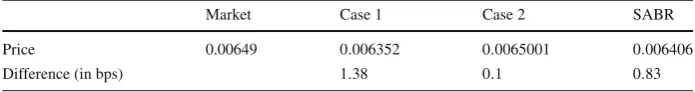
Table 3 This table presents the market price of the CMS spread against the calibrated price of the spread
using the (case 1) Black-like convexity adjustment (parallel shift), the (case 2) second convexity adjustment (tilt) and the SABR model
Market Case 1 Case 2 SABR
Price 0.00649 0.006352 0.0065001 0.006406
Difference (in bps) 1.38 0.1 0.83
The differences between the market price and the three different models are provided in basis points (bps). We
incorporate the swap spread,Xt, by assuming that the swap rate is equal to the risk-free rate plus the spread
Our numerical results suggest that in all cases market data are well reproduced. As Table2 reports, the SABR model performs slightly better than our new convexity adjustment (case 2), with 0.89 bps compared to 0.83 bps, when the spread is not taken into account, and much better compared to the Black-like formula (case 1), 0.83 bps against 2.53 bps. However, this is not the case when we take into account the swap spread. The absolute difference (in bps) between our new convexity adjustment model and the market is significantly smaller compared to the SABR case, i.e. 0.1 bps compared to 0.83 bps. Furthermore, as expected, Black’s model calibration results, although better than the non-spread case (1.38 bps against 2.53 bps), still fail to fit the data compared to the other two cases. In addition, in Table4, we report the convexity adjustments for all four cases. We observe that the convexity adjustment in the ‘tilt’ case is significantly larger than the ’flat’ case, especially, when the swap spread is incorporated. Furthermore, in the non-flat case, convexity adjustment presents a curvy shape compared to the earlier Black-like case, where the shape behaves in a more static way.
6.2 Numerical examples
[image:14.439.46.394.281.327.2]Table 4 This table presents the convexity adjustment for all four different cases, i.e. the Black-like ‘flat’ term structure with and without spread, and the ‘tilt’ term structure with and without spread
i CA (case 1) CA (case 2) CA (case 1—with spread) CA (case 2—with spread)
1 0.000036 0.000032 0.000037 0.000033
2 0.000074 0.000083 0.000076 0.000092
3 0.000114 0.000198 0.000116 0.000218
4 0.000154 0.000313 0.000158 0.000343
5 0.000196 0.000428 0.000201 0.000469
6 0.000238 0.000542 0.000245 0.000593
7 0.000282 0.000656 0.000289 0.000718
8 0.000326 0.000769 0.000335 0.000842
9 0.000373 0.000883 0.000383 0.000967
10 0.000420 0.000995 0.000431 0.001090
11 0.000468 0.001107 0.000480 0.001213
12 0.000514 0.001216 0.000528 0.001334
13 0.000564 0.001326 0.000579 0.001455
14 0.000615 0.001436 0.000631 0.001576
15 0.000667 0.001544 0.000685 0.001697
16 0.000721 0.001652 0.000739 0.001817
17 0.000775 0.001759 0.000795 0.001936
18 0.000831 0.001865 0.000852 0.002054
19 0.000888 0.001970 0.000911 0.002172
20 0.000946 0.002074 0.000970 0.002289
The whole structure from year 1 to year 20 is given
Table 5 This table reports
market CMS swap spreads (in bps) and market ATM swaption volatilities data for specific dates
Date Market CMS Market volatility (%)
10/08/2007 41.6 12.30
31/10/2008 104.5 12.98
28/05/2010 178.1 19.30
03/06/2011 136.4 19.80
09/03/2012 158.65 25.15
CMS swap spreads have cms maturity of 5 years and associated underlying swaps with maturity of 10 years
swap spreads, where the maturity of the CMS is 5 years, and the associated underlying swaps have a 10-year maturity. Furthermore, the market at-the-money swaption volatilities, for all different dates, are reported, while Table6reports market volatility smiles across different strikes and for different dates. We can observe that market data clearly show levels of turmoil in the market during the period of the financial crisis.
[image:15.439.166.394.390.472.2]Table 6 This table reports market swaption volatility smiles for different dates
Date −200 (%) −100 (%) −50 (%) −25 (%) 25 (%) 50 (%) 100 (%) 200 (%)
10/08/2007 2.75 1.01 0.44 0.20 −0.18 −0.29 −0.47 −0.70
31/10/2008 3.81 1.08 0.40 0.20 −0.20 −0.40 −0.72 −1.22
28/05/2010 8.53 3.12 1.29 0.64 −0.45 −0.86 −1.38 −2.09
03/06/2011 6.96 2.51 1.09 0.46 −0.42 −0.76 −1.22 −1.78
09/03/2012 9.61 3.02 1.23 0.56 −0.44 −0.77 −1.30 −1.81
[image:16.439.48.393.209.340.2]Strikes are expressed as absolute differences in basis points w.r.t. the ATM values
Table 7 This table presents the model parameters, obtained from the calibrated procedure, of the functions
described in Sects.3and4for the different dates in our sample
Date 10/08/2007 31/10/2008 28/05/2010 03/06/2011 09/03/2012
SABR parameters
alpha 0.0585 0.0579 0.0885 0.0912 0.1139
beta 0.7539 0.7161 0.768 0.7643 0.7794
rho −0.2341 −0.277 −0.3957 −0.3433 −0.2364
epsilon 0.1926 0.2177 0.2848 0.2867 0.231
f (Nelson–Siegel)
a 0.001 0.005 −0.03 −0.01 −0.002
b 0.002 0.0012 0.0047 0.0043 0.0038
k 0.003 0.015 0.001 0.05 0.004
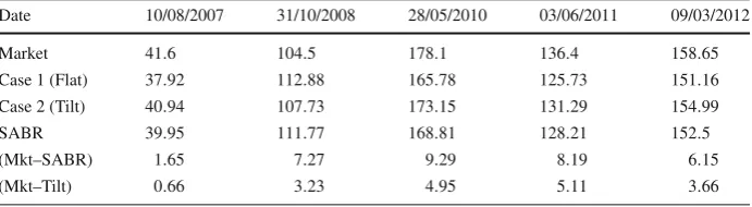
Table 8 This table compares market CMS spread prices against each different case
Date 10/08/2007 31/10/2008 28/05/2010 03/06/2011 09/03/2012
Market 41.6 104.5 178.1 136.4 158.65
Case 1 (Flat) 37.92 112.88 165.78 125.73 151.16
Case 2 (Tilt) 40.94 107.73 173.15 131.29 154.99
SABR 39.95 111.77 168.81 128.21 152.5
(Mkt–SABR) 1.65 7.27 9.29 8.19 6.15
(Mkt–Tilt) 0.66 3.23 4.95 5.11 3.66
Absolute differences (in bps) between market CMS swap spreads and the models are given
Even in the period of 2008–2011, where market was experiencing an unprecedented tur-bulence, our convexity adjustment performs well, since the difference between the market data and the SABR model is sufficiently higher than the case of the ‘tilt’ term structure, with a difference of around 3–5 basis points (for the ‘tilt’) compared to 7–9 basis points (for the SABR). Furthermore, in every case the results are in between the limits of the bid-ask spread of around 10 basis points, indicating that the market data are well recovered across all periods.
[image:16.439.48.394.375.470.2]Fig. 1 This figure shows the convexity adjustments for the ‘flat’ term structure (red), the ‘tilt’ term structure (green) and the SABR model (blue). In all cases the swap spread is taken into account. In thelower panel, the
calibrated volatility smile is displayed. Results are from a specific date, 03/02/2006. (Colour figure online)
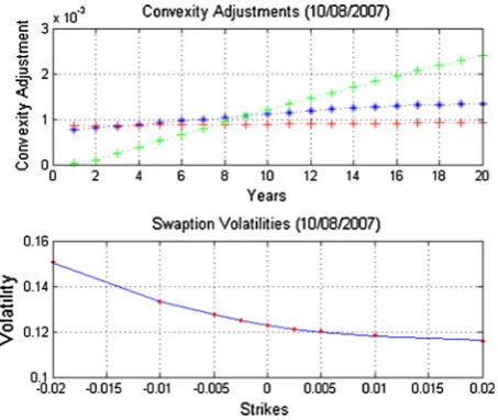
Fig. 2 This figure shows the convexity adjustments for the ‘flat’ term structure (red), the ‘tilt’ term structure
(green)and the SABR model (blue). In all cases the swap spread is taken into account. In thelower panel, the
calibrated volatility smile is displayed. Results are from a specific date, 10/08/2007. (Colour figure online)
[image:17.439.108.336.56.249.2] [image:17.439.108.335.292.483.2]Fig. 3 This figure shows the convexity adjustments for the ‘flat’ term structure (red), the ‘tilt’ term structure (green) and the SABR model (blue). In all cases the swap spread is taken into account. In thelower panel, the
calibrated volatility smile is displayed. Results are from a specific date, 31/10/2008. (Colour figure online)
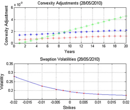
Fig. 4 This figure shows the convexity adjustments for the ‘flat’ term structure (red), the ‘tilt’ term structure
(green) and the SABR model (blue). In all cases the swap spread is taken into account. In thelower panel, the
calibrated volatility smile is displayed. Results are from a specific date, 28/05/2010. (Colour figure online)
[image:18.439.108.334.56.243.2] [image:18.439.107.335.289.481.2]Fig. 5 This figure shows the convexity adjustments for the ‘flat’ term structure (red), the ‘tilt’ term structure (green) and the SABR model (blue). In all cases the swap spread is taken into account. In thelower panel, the
calibrated volatility smile is displayed. Results are from a specific date, 03/06/2011. (Colour figure online)
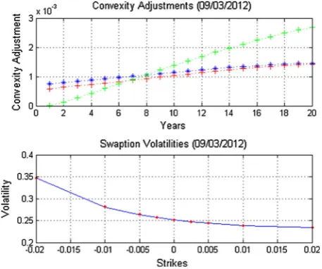
Fig. 6 This figure shows the convexity adjustments for the ‘flat’ term structure (red), the ‘tilt’ term structure
(green) and the SABR model (blue). In all cases the swap spread is taken into account. In thelower panel, the
calibrated volatility smile is displayed. Results are from a specific date, 09/03/2012. (Colour figure online)
7 Conclusion
[image:19.439.108.335.55.247.2] [image:19.439.106.335.292.483.2]curves, which clearly, can no longer be based on traditional bootstrapping procedures. In that vein, our work fills the gap of the shortcomings of single yield curve model adjustments, widely used in the literature, when one deals with the issue of convexity in money market instruments.
In the double-curving environment that we describe, we have derived the convexity factor requirement in the conventional case that the term structure of interest rates is flat, and its dynamic evolution allows only for parallel shifts, and we have expanded our setting to incorporate the more realistic and challenging case of term structure tilts. The new term appears to be approximately linear in this parameter. In all computations, our results conclude that the convexity adjustment of the ‘tilt’ term structure case is significantly larger than the convexity adjustments implied by the Black and SABR models.
As an empirical illustration, we have calibrated both convexity adjustments to real market data, by using swaption volatilities, and calculated the differences between market quotes and our model implied CMS spreads. We further compared our results with the widely used by market practitioners smile-consistent CMS adjustment, using the SABR model. We con-sidered a different SABR model for each swap rate contained in the CMS payoff, and we performed a calibration of all the SABR parameters to swaption volatility smile and CMS spreads quoted by the market. In all cases the swaption volatility smiles are very well recov-ered by the calibrated SABR models. Furthermore, our results demonstrate that the proposed convexity adjustments offer a market consistent and robust valuation of CMS spreads, and suggest that CMS-type of products should be priced under a multi-curve framework.
Open Access This article is distributed under the terms of the Creative Commons Attribution 4.0
Interna-tional License (http://creativecommons.org/licenses/by/4.0/), which permits unrestricted use, distribution, and
reproduction in any medium, provided you give appropriate credit to the original author(s) and the source, provide a link to the Creative Commons license, and indicate if changes were made.
Appendix 1: Expectation of swap rate and spread
To calculateEQtid,j
STti−1,j
i−1 XTi−1 , we letYt =ln(S ti−1,j
t Xt), and we apply Ito’s Lemma.
dYt = ∂
Yt
∂Stti−1,jd S
ti−1,j
t +
∂Yt
∂Xt
d Xt+ 1 2
∂2Y
t
∂Stti−1,j
d Stti−1,j
2
+1 2
∂2Y
t
∂Xt2(d Xt)
2+ ∂2Yt
∂Stti−1,j∂Xt
d Stti−1,jd Xt =σt,Sd Wt,S+σt,Xd Wt,X−
1 2
(σt,S)2+(σt,X)2
dt (42)
So,
dln
Stti−1,jXt
=σt,Sd Wt,S+σt,Xd Wt,X− 1 2
(σt,S)2+σt2,X
dt (43)
which means that,
StTi−1,j
i−1 XTi−1 =S ti−1,j
t Xte− 1 2
(σt,S)2+σt2,X (Ti−1−t)e
So,
EQtid,j Sti−1,j
Ti−1 XTi−1 =E Qtid,j
Stti−1,jXte− 1 2
(σt,S)2+σt2,X (Ti−1−t)
×EQtid,j eσt,SW(Ti−1−t),S+σt,XW(Ti−1−t),X (45)
In general, if: X ∼ N(0, σX2),Y ∼ N(0, σY2)andE[eX+Y], then we have, E[e12var(X+Y)] withvar(X+Y)=var(X)+var(Y)+2ρ√var(X)var(Y)
So, in our case,
X =σt,SW(Ti−1−t),S ∼N
0, (σt,S)2(Ti−1−t)
(46)
Y =σt,XW(Ti−1−t),X ∼N
0, σt2,X(Ti−1−t)
(47)
var(X+Y)=(σt,S)2(Ti−1−t)+σt2,X(Ti−1−t)+2ρs,x
+
(σt,S)2tσt2,Xt
=(σt,S)2(Ti−1−t)+σt2,X(Ti−1−t)+2ρs,xσt,Sσt,X(Ti−1−t) (48) So,
EQtid,j eσt,SW(Ti−1−t),S+σt,XW(Ti−1−t),X =EQtid,j
e
1 2
(σt,S)2+σt2,X+2ρs,xσt,Sσt,X
(Ti−1−t)
(49)
So, finally,
EQtid,j Sti−1,j
Ti−1 XTi−1 =S ti−1,j
t Xteρs,xσt,Sσt,X(Ti−1−t) (50)
Appendix 2: Partial derivatives
Calculation of partial derivatives: Gr(r,t)
G(r,t) andGGt((rr,,tt)). We start with our function,
G(r,t)=
1+τfTi
t (r)
−(Ti−t) τ
c
j=1τ
1+τftti,j(r)
−(ti,j−t) τ
(51)
and let,
u=
1+τfTi
t (r)
−(Ti−t)
τ
(52)
v= c
j=1
τ1+τftti,j(r)
−(ti,j−t)
τ
(53)
So,
∂u
∂r = −(Ti−t)
1+τfTi
t (r)
−(Ti−t)
τ −1 ∂ftTi(r)
∂r (54)
∂v ∂r =
c
j=1
τ(−(ti,j−t))
1+τftti,j(r)
−(ti,j−t)
τ −1 ∂ftti,j(r)
So,
Gr(r,t)=
−(Ti−t)
1+τfTi
t (r) −(Ti−t)
τ −1∂fTi
t (r)
∂r c
j=1τ
1+τftti,j(r)−
(ti,j−t)
τ
+
1+τfTi
t (r) −(Tiτ−t) c
j=1τ
1+τftti,j(r) −(ti,j−t)
τ
c
j=1τ(ti,j−t)
1+τftti,j(r)−
(ti,j−t)
τ −1∂fti,j t (r)
∂r c
j=1τ
1+τftti,j(r) −(ti,j−t)
τ
(56)
and if we divide each term withG(r,t), we have,
Gr(r,t)
G(r,t) =
−(Ti−t) 1+τfTi
t (r)
∂fTi
t
∂r (r)+
c
j=1(ti,j−t)(1+τf ti,j
t (r))−
ti,j−t
τ −1∂f
ti,j t
∂r (r)
c
j=1(1+τf
ti,j
t (r))−
ti,j−t
τ
(57)
For the partial derivative with respect tot,Gt(r,t), we proceed as before,
∂u
∂t =
1+τfTi
t (r)
−(Ti−t) τ
−(Ti−t) 1+τfTi
t (r)
∂fTi
t
∂t (r)+
1
τ ln
1+τfTi
t (r)
(58)
∂v ∂t =
c
j=1
τ1+τftti,j(r)
−(ti,j−t)
τ
1
τ ln
1+τftti,j(r)
− (ti,j−t) 1+τftti,j(r)
∂ftti,j
∂t (r)
(59)
So:
Gt(r,t)=
1+τfTi
t (r)
−(Ti−t)
τ −(Ti−t)
1+τftTi(r) ∂ftTi
∂t (r)+
1
τln(1+τftTi(r))
c j=1τ
1+τftti,j(r)
−(ti,j−t)
τ
−
1+τfTi
t (r)
−(Ti−t) τ
c j=1τ
1+τftti,j(r)
−(ti,j−t)
τ
×
c j=1τ
1+τftti,j(r)
−(ti,j−t)
τ 1
τln(1+τf
ti,j
t (r))− ( ti,j−t)
1+τftti,j(r)
∂ftti,j
∂t (r)
c
j=1τ
1+τftti,j(r)
−(ti,j−t) τ
(60)
So, if we divide each term withG(r,t), we have,
Gt(r,t)
G(r,t) =
1
τ ln
1+τfTi
t (r)
− Ti−t
1+τfTi
t (r)
∂fTi
t
−
c j=1
1+τftti,j(r)
−(ti,j−t)
τ 1
τ ln
1+τftti,j(r)
− (ti,j−t)
1+τftti,j(r)
∂ftti,j
∂t (r)
c j=1
1+τftti,j(r)
−(ti,j−t) τ
(61)
References
Ametrano, F., & Bianchetti, M. (2009).Bootstrapping the illiquidity: Multiple yield curves construction for
market coherent forward rates estimation. London: Risk Books, Incisive Media.
Bianchetti, M. (2010). Two curves, one price: Pricing and hedging interest rate derivatives using different yield curves for discounting and forwarding. preprint. Available at SSRN 1334356
Boenkost, W., & Schmidt, W. (2005). Cross currency swap valuation. Available at SSRN 1375540.
Brigo, D., & Mercurio, F. (2006).Interest rate models-theory and practice: With smile, inflation and credit.
New York: Springer.
Chibane, M., & Sheldon, G. (2009). Building curves on a good basis. Available at SSRN 1394267 Crépey, S., Grbac, Z., Ngor, N., & Skovmand, D. (2015). A lévy hjm multiple-curve model with application
to cva computation.Quantitative Finance,15(3), 401–419.
Crépey, S., Grbac, Z., & Nguyen, H. N. (2012). A multiple-curve hjm model of interbank risk.Mathematics
and Financial Economics,6(3), 155–190.
Cuchiero, C., Fontana, C., & Gnoatto, A. (2016). A general hjm framework for multiple yield curve modelling.
Finance and Stochastics,20(2), 267–320.
Fanelli, V. (2016). A defaultable HJM modelling of the libor rate for pricing basis swaps after the credit crunch.
European Journal of Operational Research,249(1), 238–244.
Filipovi´c, D., & Trolle, A. B. (2013). The term structure of interbank risk.Journal of Financial Economics,
109(3), 707–733.
Fujii, M., Shimada, Y., & Takahashi, A. (2010). On the term structure of interest rates with basis spreads, collateral and multiple currencies. Available at SSRN 1556487
Grbac, Z., Papapantoleon, A., Schoenmakers, J., & Skovmand, D. (2015). Affine libor models with multiple
curves: Theory, examples and calibration.SIAM Journal on Financial Mathematics,6(1), 984–1025.
Hagan, P. S. (2005).Convexity conundrums: Pricing CMS swaps, caps, and floors.In The best of Wilmott,
305. Chichester: Wiley.
Hagan, P. S., Kumar, D., Lesniewski, A. S., & Woodward, D. E. (2002). Managing smile risk. Wilmott
Magazine, pp. 84–108.
Henrard, M. (2007a). CMS swaps in separable one-factor Gaussian LLM and HJM model. Bank for Interna-tional Settlements, Working Paper
Henrard, M. (2007b).The irony in the derivatives discounting. Wilmott Magazine, Jul/Aug.
Henrard, M. (2010). The irony in derivatives discounting part II: The crisis.Wilmott Journal,2(6), 301–316.
Kijima, M., Tanaka, K., & Wong, T. (2009). A multi-quality model of interest rates.Quantitative Finance,
9(2), 133–145.
Liu, J., Longstaff, F. A., & Mandell, R. E. (2006). The market price of risk in interest rate swaps: The roles of
default and liquidity risks.The Journal of Business,79(5), 2337–2359.
Lu, Y., & Neftci, S. (2003). Convexity adjustment and forward libor model: Case of constant maturity swaps. Technical report, FINRISK-Working Paper Series.
Mercurio, F. (2009). Interest rates and the credit crunch: New formulas and market models. Bloomberg Portfolio Research Paper (2010-01).
Mercurio, F. (2010). Libor market models with stochastic basis. Bloomberg Education and Quantitative Research Paper (2010-05).
Mercurio, F., & Pallavicini, A. (2005). Swaption skews and convexity adjustments. Banca IMI, SSRN Working Paper.
Mercurio, F., & Pallavicini, A. (2006). Smiling at convexity: Bridging swaption skews and CMS adjustments. Risk August, pp. 64–69.
Moreni, N., & Pallavicini, A. (2014). Parsimonious HJM modelling for multiple yield curve dynamics.
Quan-titative Finance,14(2), 199–210.
Pallavicini, A., & Tarenghi, M. (2010). Interest-rate modeling with multiple yield curves. Available at SSRN 1629688.
Pelsser, A. (2003). Mathematical foundation of convexity correction.Quantitative Finance,3(1), 59–65.
Wu, T. P., & Chen, S. N. (2010). Modifying the LMM to price constant maturity swaps.Journal of Derivatives,
18(2), 20.
Zheng, W., & Kuen Kwok, Y. (2011). Convexity meets replication: Hedging of swap derivatives and annuity