A Compact Geometrically Nonlinear FE Shell Code for Cardiac Analysis: Shell Formulation

City, University of London Institutional Repository

Citation

: Wong, Y. and Crouch, R.S. (2018). A Compact Geometrically Nonlinear FE Shell

Conference on Computational Mechanics (ECCM 6), 11-15 Jun 2018, Glasgow, UK.

This is the accepted version of the paper.

This version of the publication may differ from the final published

version.

Permanent repository link:

Link to published version

:

Copyright and reuse:

City Research Online aims to make research

outputs of City, University of London available to a wider audience.

Copyright and Moral Rights remain with the author(s) and/or copyright

holders. URLs from City Research Online may be freely distributed and

linked to.

City Research Online: http://openaccess.city.ac.uk/ [email protected]

1115 June 2018, Glasgow, UK

A COMPACT GEOMETRICALLY NONLINEAR FE SHELL

CODE FOR CARDIAC ANALYSIS: SHELL FORMULATION

YEW YAN WONG AND ROGER S CROUCH

City, University of London 10 Northampton Square, EC1V 8EN

[email protected]

Key words: Cardiac Analysis, Shell Finite Elements, Large Deformations

Abstract. There are few free open-source FE programs for 3D geometrically nonlinear shell elements that allow users to modify or extend the code. This paper presents such a MATLAB code which draws heavily on the work of Coombs1 _{and Coombs et al}2_.

1 INTRODUCTION

Cardiovascular disease is the largest cause of death in humans and account for 45% of all loss of life in Europe in 20173_{; with cardiac arrhythmias being the most}

trouble-some medical condition. The cause of cardiac arrhythmias is still not that well understood. Clinical studies are impeded by invasive and expensive in-vivo cardiac experimentation4,5_.

As an alternative approach, mathematical modelling6,7,8 _{coupled with the advancement}

in high-resolution MRI scans are increasingly being used to assist in the study of cardiac behaviour9,10,11,12_{. However, these simulations can be computationally expensive.}

Consid-erable effort has been put into trying to optimise analyses by taking advantage of parallel processors4,5. Yet a recent analysis with 60 million degrees of freedom still required 50 minutes of run time to compute a single cardiac cycle with 127 Xeon processor cores when using conventional 3D solid finite elements12_.

Lack of open source codes hinders research development in the field. The study de-scribed here makes use of shell finite elements which reduces the requirement for many hexahedra or tetrahedral elements through the thickness of the heart muscle walls. In this paper, a compact three dimensional MATLAB code forTotal-Lagrangian Finite Element Analyses (FEA) using 9-noded shell elements, is presented. Code performance is com-pared here against hexahedral2 _{elements using a cantilever subjected to a transverse end}

2 METHODS

2.1 Electro-mechanical coupling

Cardiac muscle tissue is highly orientated, with muscle fibres aligned in near-parallel bundles. These fibres contract and relax following changes in the electrical membrane po-tential. The latter can be modelled by two different means; (i) use of localionic concentra-tion models, which account for the intracellular movement of ions or (ii) phenomenolog-ical models which duplicate the membrane potential behaviour seen in electrocardiogram

(ECG) scans. The second approach allows for significant savings on computational time. A one-dimensional coupled electro-mechanical finite difference code that propagates the membrane potential through a monodomain model has already been constructed by the first author. This is currently being extended to the shell element formulation.

2.2 Formulation of the Total-Lagrangian approach for shell elements

The key concept of the continuum based degenerated shell finite element formulation is to capture information of the through-thickness bending behaviour by the intrudction of rotational degree of freedoms. The 3D coordinate field is given as follows14_:

_t

x =

N

X

k=1

hktxk +ζ 2

N

X

k=1

akhktV_nk (1)

where ζ gives the local coordinates of the z−axis,{t_xk_{}, h}k_{, a}k _and{t_Vk

n}is the

coor-dinates,shape functions (made-up of membrane local coordinates ξ andη), the thickness of the shell and the thickness direction vectors at node k (N being the total number of nodes in the elements) at time t respectively. Two different angles (θx and θy) are used

to identify the initial thickness direction vector with respect to the global x−axis and

y−axis at each node. The initial thickness direction vector can then be expressed as:

₀

Vk n =

 



cos(θk x)

sin(θk

x) cos(θky)

sin(θ_xk) sin(θk_y)  



(2)

The displacements are given by {u} ={t+∆t_{x} − {}t_{x}. The thickness direction vector}

can be expressed in terms of a rotation about the x−axis α, and a rotation about the

y−axis, β as {t_Vk

n}=−{tV2k}αk+{tV1k}βk. Thus, the displacement becomes:

_t

u =

N

X

k=1

hktuk +ζ 2

N

X

k=1

akhk(−αk{t_Vk

2 }+β

k_{t_Vk

1 }) (3)

When large deformation and rotation arise in a geometrically nonlinear FEA, the

constitutive matrix [D], is updated in order to follow the deformed configuration by means of a rotation matrix [Q], which is recorded in equations (5.119) and (5.120) in the work by Bathe15.

 



ui,t_x

1

ui,t_x

2

ui,t_x

3    =    ∂ui

∂t_x

1

∂ui

∂t_x

2

∂ui

∂t_x

3    = N X k=1   t_h

k,1 tgk1itG1k tgk2itGk1

t_h

k,2 tgk1itG2k tgk2itGk2

t_h

k,3 tgk1itG3k tgk2itGk3

     uk i αk βk    (4)

where {thk}, {g1k} and {gk2} and {tGk} are defined below.

_t

hk =

  

 

(t_J−1₎ 11dN

k

dξ + ( t_J−1₎

12dN

k

dη

(t_J−1₎ 21dN

k

dξ + ( t_J−1₎

22dN

k

dη

(t_J−1₎ 31dN

k

dξ + ( t_J−1₎

32dN k dη      _t gk

1 =−

1 2a

k_t

Vk 2 _t gk 2 = 1 2a

k_t

Vk

1

_t

Gk =t

        

ζ(t_J−1₎ 11dN

k

dξ + ( t_J−1₎

12dN

k

dη

+ (t_J−1₎ 13Nk

ζ(tJ−1)21dN

k

dξ + ( t_J−1₎

22dN

k

dη

+ (tJ−1)23Nk

ζ(t_J−1₎ 31dN

k

dξ + ( t_J−1₎

32dN

k

dη

+ (t_J−1₎ 33Nk

         (5)

InTotal-Lagrangian formulations, theGreen-Lagrange strain can be divided into linear and nonlinear components as shown in equation (19) of Bathe et al16_{. To take into}

account of this, the strain-displacement matrix is divided into a linear component [BL],

and a nonlinear component [BN L], which can both be found in Table 4 of Bathe and

Bolourchi14 _(as t

0BL0 and t0BL1 respectively). However, the nonlinear strain-displacement

matrix work reported here is computed by obtaining the product of an auxiliary matrix [A] (expressed in equation (7.24) of Stegmann16) and the nonlinear strain-displacement transformation matrix, [GN L] known ast0BN L by Bathe and Bolourchi14 in Table 4 or [G]

in equation (7.26) by Stegmann16_.

TheGreen-Lagrange strain{}, can then be determined as{}={n_}+{t_{}, where{}n_}

is the strain state corresponding to the previous iteration and{t_{}is the strain increment.}

The strain increment can determined as shown in Table 6.2 (as 0eij) by Bathe14. The

second-Piola Kirchoff stress can now determined from as {σ}= {n_{σ}+ [D}

sh]{t}, where

[Dsh] is the constitutive matrix of the deformed configuration13.

Having formed the strain-displacement matrix, [B], the constitutive matrix, [Dsh] and

the nonlinear strain-displacement transformation matrix, [GN L], the tangent stiffness

ma-trix, [Ke] can now be computed as:

Ke = nGp X i=1

[B]T[Dsh][B] + [GN L]T[H][GN L]

|J|wi (6)

where |J| is the determinant of the Jacobian and wi is the Gauss weighting for Gauss

point i. The nodal internal force can now be determined as:

fint = nGp

X

i=1

BT σ J

w_i (7)

foob =

fext +

frct −

fint (8)

If this out-of-balance force is within a pre-defined tolerance, then that load step is deemed to have converged and the analysis moves on to the next load step. However, if it is not within the tolerance, the displacement is updated by determining the displacement variation {δu} by making use ofNewton Raphson iterations with a new tangent stiffness matrix and the out-of-balance force.

K δu =foob (9)

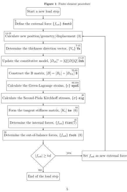
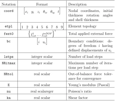
The procedure of the FEA and the variable update sequence is summarised in Figure 1. The number in the top left of each process refers to the line number of the main MATLAB script (Listing 1) whereas the number in the top right refers to the line number of the MATLAB function files (Listing 2).

The parameters required to define the problem and the initial geometry needs to be stored in a M-script inputfile.m with the parameters explained in Table 1 below.

Table 1: inputfile.m parameters

Notation Format Description

coord

h

xi yi zi θix θiy t

i

Nodal coordinates, initial thickness rotation angles and shell thickness

etpl

h

1 2 3 4 5 6 7 8 9 i

Element topology

fext0

n

f1

ext. . . fextnDOF

oT

Total applied external force

bc

h

i ui

i

Boundary conditions: de-grees of freedom i having defined displacements ofui

lstps integer scalar Number of load steps

NRitmax integer scalar Maximum number of itera-tions per load step

NRtol real scalar Out-of-balance force

toler-ance for convergence

E real scalar Young’s modulus (Pascal)

nu real scalareger Poisson’s ratio

Figure 1: Finite element procedure

Start a new load step

Define the external force {fext} fext0

Calculate new position/geometry/displacement (3)

Determine the thickness direction vector, {Vn} Vn

Update the constitutive model, [Dsh]T= [Q][D][Q] Dsh

Construct the B matrix, [B] = [BL] + [BN L] B

Calculate the Green-Lagrange strains, {} epsE

Calculate the Second-Piola Kirchhoff stresses, {σ}sig

Form the tangent stiffness matrix, [Ke] ke (6)

Determine the internal forces, {fint} fint(7)

Determine the out-of-balance forces, {foob} foob (8)

|foob| ≥tol Set foob as new external force

End of the load step

yes

no

9

14-19

7-15

17-37

55-92

93-104

40

44

45

1 [ coord , etpl , fext0 , bc , lstps , NRitmax , NRtol , E , nu , ka ]= i n p u t f i l e ; 2 n e l s =s i z e( etpl ,1) ; n o d e s =s i z e( coord ,1) ; n D o F = n o d e s *5;

3 n e D o F = ( 9 * 5 ) ^2; k r o w =z e r o s( n e D o F * nels ,1) ; k c o l = k r o w ; k v a l = k r o w ; 4 uvw =z e r o s( nDoF ,1) ; u v w o l d = uvw ; f i n t = uvw ; r e a c t = uvw ;

5 fd = ( 1 : n D o F ) ; fd ( bc (: ,1) ) = [ ] ;

6 e p s E n =z e r o s(6 ,8 , n e l s ) ; e p s E = e p s E n ; s i g N = e p s E n ; sig = e p s E n ; 7 Vn =z e r o s(9 ,3 , n e l s ) ; oVn = Vn ; oL =z e r o s(8 ,9 , n e l s ) ; L = oL ; 8 for l s t p =0: l s t p s

9 f e x t =( l s t p / l s t p s ) * f e x t 0 ; f o o b = r e a c t + fext - f i n t ;

10 f o o b n o r m =2* N R t o l ; N R i t =0;

11 w h i l e (( NRit < N R i t m a x ) &&( f o o b n o r m > N R t o l ) )

12 N R i t = N R i t +1; f i n t =z e r o s( nDoF ,1) ; d r e a c t = f i n t ; d d u v w = f i n t ;

13 if lstp >=1

14 Kt =s p a r s e( krow , kcol , kval , nDoF , n D o F ) ;

15 d d u v w ( bc (: ,1) ) = ( 1 +s i g n(1 - N R i t ) ) * bc (: ,2) / l s t p s ;

16 d d u v w ( fd ) = Kt ( fd , fd ) \( f o o b ( fd ) - Kt ( fd , bc (: ,1) ) * d d u v w ( bc (: ,1) ) ) ; 17 d r e a c t ( bc (: ,1) ) = Kt ( bc (: ,1) ,:) * dduvw - f o o b ( bc (: ,1) ) ;

18 end

19 uvw = uvw + d d u v w ; r e a c t = r e a c t + d r e a c t ; d u v w = uvw - u v w o l d ;

20 for nel =1: n e l s

21 ed =r e s h a p e( o n e s (5 ,1) * e t p l ( nel ,:) *5 -(5 -1: -1:0) . ’* o n e s (1 ,9) ,1 ,9*5) ;

22 if l s t p ==0

23 e l c o o r d = c o o r d ( e t p l ( nel ,:) ,:) ;

24 phi = e l c o o r d (: ,4) ; psi = e l c o o r d (: ,5) ;

25 oVn (: ,: , nel ) =[cos( psi ) sin( psi ) .*cos( phi ) sin( psi ) .*sin( phi ) ];

26 end

27 [ ke , felem , e p s E (: ,: , nel ) , Vn (: ,: , nel ) , sig (: ,: , nel ) , L (: ,: , nel ) ] = . . . 28 s h e l l ( c o o r d ( e t p l ( nel ,:) ,:) , uvw ( ed ) , d u v w ( ed ) , e p s E n (: ,: , nel ) ,... 29 oVn (: ,: , nel ) ,E , nu , ka , s i g N (: ,: , nel ) , oL (: ,: , nel ) ) ;

30 if l s t p ==0

31 ct =( nel -1) * n e D o F +1: nel * n e D o F ;

32 k r o w ( ct ) =r e s h a p e( ed . ’* o n e s (1 ,9*5) , neDoF ,1) ; 33 k c o l ( ct ) =r e s h a p e( o n e s (9*5 ,1) * ed , neDoF ,1) ;

34 end

35 k v a l (( nel -1) * n e D o F +1: nel * n e D o F ) =r e s h a p e( ke , neDoF ,1) ; 36 f i n t ( ed ) = f i n t ( ed ) + f e l e m ;

37 end

38 f o o b = f e x t + react - f i n t ; f o o b n o r m =n o r m( f o o b ) /n o r m( f e x t + r e a c t +eps) ; 39 f p r i n t f(’ %4 i %4 i % 6 . 3 e \ n ’, lstp , NRit , f o o b n o r m ) ;

40 end

41 u v w o l d = uvw ; e p s E n = e p s E ; s i g N = sig ; oL = oL + L ; 42 end

1 f u n c t i o n [ ke , fint , epsE , Vn , sig , L ]= s h e l l ( n o d e D a t a , uvw , duvw , epsEn , oVn , . . .

2 E , nu , ka , sigN , oL )

3 c o o r d = n o d e D a t a (: ,1:3) ; t = n o d e D a t a (: ,6) ; e p s E =z e r o s(6 ,8) ;

4 ke =z e r o s( 9 * 5 ) ; f i n t =z e r o s(9*5 ,1) ; dxr =z e r o s(3) ; [ wp , G p L o c ]= G p P o s () ;

5 ex =[1 0 0]. ’; ey =[0 1 0]. ’; ez =[0 0 1]. ’;

6 V1 =z e r o s(9 ,3) ; V2 = V1 ; g1 = V1 ; g2 = V1 ;

7 xsi =[ -1; -1; -1; 0; 1; 1; 1; 0; 0]; eta =[ -1; 0; 1; 1; 1; 0; -1; -1; 0];

8 dNr = d e r s h a p e f u n c ( xsi , eta ) ; dnr = dNr ( 1 : 2 :end,:) ; dns = dNr ( 2 : 2 :end,:) ; 9 dsp =r e s h a p e( uvw - duvw ,5 ,[]) ’; e l c o o r d = c o o r d + dsp (: ,1:3) ;

10 for n = 1 : 9

11 Vn ( n ,:) =c r o s s(( dnr ( n ,:) * e l c o o r d ) /n o r m( dnr ( n ,:) * e l c o o r d ) ,... 12 ( dns ( n ,:) * e l c o o r d ) /n o r m( dns ( n ,:) * e l c o o r d ) ) ; 13 V =c r o s s( ey , Vn ( n ,:) . ’) . ’;

14 V1 ( n ,:) = V /n o r m( V ) ; V2 ( n ,:) =c r o s s( Vn ( n ,:) . ’ , V1 ( n ,:) . ’) . ’; 15 g1 ( n ,:) = -0.5* t ( n ) * V2 ( n ,:) ; g2 ( n ,:) = 0 . 5 * t ( n ) * V1 ( n ,:) ; 16 end

17 D = [ [ 1 nu ; nu 1; 0 0] z e r o s(3 ,4) ; z e r o s(3) eye(3) * ka *(1 - nu ) * 0 . 5 ] ; 18 D =( E /(1 - nu ^2) ) * D ; D (4 ,4) = D (4 ,4) / ka ;

19 for Gp = 1 : 8

20 xsi = G p L o c ( Gp ,1) ; eta = G p L o c ( Gp ,2) ; zet = G p L o c ( Gp ,3) ; 21 N = s h a p e f u n c ( xsi , eta ) ; dNr = d e r s h a p e f u n c ( xsi , eta ) ;

22 dxr (1:2 ,:) =( dNr *( c o o r d + 0 . 5 * zet *( oVn .*( t * o n e s (1 ,3) ) ) ) ) ; 23 dxr (3 ,:) = ( 0 . 5 * ( N .* t ’) * oVn ) ; V n G p =( N * oVn ) . ’;

24 s d i r = dxr (: ,2) /n o r m( dxr (: ,2) ) ;

25 er =c r o s s( sdir , V n G p ) ; er = er /n o r m( er ) ; 26 es =c r o s s( VnGp , er ) ; es = es /n o r m( es ) ; 27 et = V n G p /n o r m( V n G p ) ;

28 l1 =( ex . ’* er ) ; m1 =( ey . ’* er ) ; n1 =( ez . ’* er ) ; 29 l2 =( ex . ’* es ) ; m2 =( ey . ’* es ) ; n2 =( ez . ’* es ) ; 30 l3 =( ex . ’* et ) ; m3 =( ey . ’* et ) ; n3 =( ez . ’* et ) ;

31 Q =[ l1 * l1 m1 * m1 n1 * n1 l1 * m1 m1 * n1 n1 * l1 ;

32 l2 * l2 m2 * m2 n2 * n2 l2 * m2 m2 * n2 n2 * l2 ;

33 l3 * l3 m3 * m3 n3 * n3 l3 * m3 m3 * n3 n3 * l3 ;

34 2* l1 * l2 2* m1 * m2 2* n1 * n2 l1 * m2 + l2 * m1 m1 * n2 + m2 * n1 n1 * l2 + n2 * l1 ; 35 2* l2 * l3 2* m2 * m3 2* n2 * n3 l2 * m3 + l3 * m2 m2 * n3 + m3 * n2 n2 * l3 + n3 * l2 ; 36 2* l3 * l1 2* m3 * m1 2* n3 * n1 l3 * m1 + l1 * m3 m3 * n1 + m1 * n3 n3 * l1 + n1 * l3 ]; 37 Dsh = Q . ’* D * Q ;

38 [ B , GNL , epsEt , L ( Gp ,:) , d e t J ]= f o r m B ( G p L o c ( Gp ,:) , coord , oVn , t , g1 , g2 , . . .

39 duvw , oL ( Gp ,:) ) ;

40 e p s E (: , Gp ) = e p s E n (: , Gp ) + e p s E t ; sig (: , Gp ) = s i g N (: , Gp ) +( Dsh * e p s E t ) ; 41 H =[ sig (1 , Gp ) *eye(3) sig (4 , Gp ) *eye(3) sig (6 , Gp ) *eye(3) ;

42 sig (4 , Gp ) *eye(3) sig (2 , Gp ) *eye(3) sig (5 , Gp ) *eye(3) ; 43 sig (6 , Gp ) *eye(3) sig (5 , Gp ) *eye(3) sig (3 , Gp ) *eye(3) ]; 44 ke = ke +(( B . ’* Dsh * B ) +( GNL . ’* H * GNL ) ) * d e t J * wp ( Gp ) ;

45 f i n t = f i n t + B . ’* sig (: , Gp ) * d e t J * wp ( Gp ) ; 46 end

47

48 f u n c t i o n [ wp , G p L o c ]= G p P o s ()

49 wp = o n e s (8 ,1) ; g2 =1/s q r t(3) ; xsi =[ -1 -1 1 1 -1 -1 1 1]. ’* g2 ;

50 eta =[ -1 -1 -1 -1 1 1 1 1]. ’* g2 ; zet =[ -1 1 1 -1 -1 1 1 -1]. ’* g2 ;

53 f u n c t i o n [ B , GNL , epsEt , L , d e t J ]= f o r m B ( GpLoc , coord , Vn , t , g1 , g2 , duvw , oL ) 54 xsi = G p L o c (1) ; eta = G p L o c (2) ; zet = G p L o c (3) ;

55 N = s h a p e f u n c ( xsi , eta ) ; dNr = d e r s h a p e f u n c ( xsi , eta ) ; dxr =z e r o s(3) ; 56 dxr (1:2 ,:) =( dNr *( c o o r d + 0 . 5 * zet *( Vn .*( t * o n e s (1 ,3) ) ) ) ) ;

57 dxr (3 ,:) = ( 0 . 5 * ( N .* t ’) * Vn ) ;

58 d e t J =det( dxr ) ; i n v J =inv( dxr ) ; dNx = dxr \[ dNr ; z e r o s(1 ,9) ]; 59 G = zet *( i n v J (: ,1:2) * dNr ) + i n v J (: ,3) * N ;

60 B9 =z e r o s(9 ,9*5) ; BNL =z e r o s(6 ,9*5) ; GNL = B9 ; L =z e r o s(1 ,9) ; 61 B9 ([1 4 9] ,1:5:end) = dNx ; B9 ([5 2 6] ,2:5:end) = dNx ;

62 B9 ([8 7 3] ,3:5:end) = dNx ;

63 B9 (: ,4:5:end) = g1 (: ,[1 2 3 1 2 2 3 3 1]) ’.* G ([1 2 3 2 1 3 2 1 3] ,:) ; 64 B9 (: ,5:5:end) = g2 (: ,[1 2 3 1 2 2 3 3 1]) ’.* G ([1 2 3 2 1 3 2 1 3] ,:) ; 65 BL = B9 ( [ 1 : 3 5 7 9] ,:) ; BL (4:6 ,:) = BL (4:6 ,:) + B9 ([4 6 8] ,:) ;

66 for n = 1 : 3

67 ct = 3 * ( n -1) + 1 : 3 * ( n -1) +3; 68 for m = 1 : 9

69 m5 = 5 * ( m -1) ;

70 L (: , ct ) = L (: , ct ) +([ dNx (: , m ) g1 ( m , n ) .* o n e s (3 ,1) .* G (: , m ) ...

71 g2 ( m , n ) .* o n e s (3 ,1) .* G (: , m ) ]*[ d u v w (( m5 ) + n ) ;

72 d u v w (( m5 ) +4) ; d u v w (( m5 ) +5) ]) ’;

73 end 74 end 75 tL = oL + L ;

76 A =[ tL ( : , 1 : 3 : 9 ) z e r o s(1 ,3) z e r o s(1 ,3) ;

77 z e r o s(1 ,3) tL ( : , 2 : 3 : 9 ) z e r o s(1 ,3) ; 78 z e r o s(1 ,3) z e r o s(1 ,3) tL ( : , 3 : 3 : 9 ) ; 79 tL ( : , 2 : 3 : 9 ) tL ( : , 1 : 3 : 9 ) z e r o s(1 ,3) ; 80 z e r o s(1 ,3) tL ( : , 3 : 3 : 9 ) tL ( : , 2 : 3 : 9 ) ; 81 tL ( : , 3 : 3 : 9 ) z e r o s(1 ,3) tL ( : , 1 : 3 : 9 ) ]; 82 for n = 1 : 9

83 ct = 5 * ( n -1) + 1 : 5 * ( n -1) +5;

84 GNL (: , ct ) =[ dNx (1 , n ) *eye(3) g1 ( n ,:) ’.* G (1 , n ) .* o n e s (3 ,1) ...

85 g2 ( n ,:) ’.* G (1 , n ) .* o n e s (3 ,1) ;

86 dNx (2 , n ) *eye(3) g1 ( n ,:) ’.* G (2 , n ) .* o n e s (3 ,1) ...

87 g2 ( n ,:) ’.* G (2 , n ) .* o n e s (3 ,1) ;

88 dNx (3 , n ) *eye(3) g1 ( n ,:) ’.* G (3 , n ) .* o n e s (3 ,1) ...

89 g2 ( n ,:) ’.* G (3 , n ) .* o n e s (3 ,1) ];

90 BNL (: , ct ) = A * GNL (: , ct ) ; 91 end

92 B = BL + BNL ;

105 f u n c t i o n [ N ]= s h a p e f u n c ( xsi , eta )

106 N (: ,1) = xsi .*( xsi -1) .* eta .*( eta -1) /4; 107 N (: ,2) = - xsi .*( xsi -1) .*( eta +1) .*( eta -1) /2; 108 N (: ,3) = xsi .*( xsi -1) .* eta .*( eta +1) /4; 109 N (: ,4) = -( xsi +1) .*( xsi -1) .* eta .*( eta +1) /2; 110 N (: ,5) = xsi .*( xsi +1) .* eta .*( eta +1) /4; 111 N (: ,6) = - xsi .*( xsi +1) .*( eta +1) .*( eta -1) /2; 112 N (: ,7) = xsi .*( xsi +1) .* eta .*( eta -1) /4; 113 N (: ,8) = -( xsi +1) .*( xsi -1) .* eta .*( eta -1) /2;

114 N (: ,9) =( xsi +1) .*( xsi -1) .*( eta +1) .*( eta -1) ; 115

116 f u n c t i o n [ dNr ]= d e r s h a p e f u n c ( xsi , eta ) 117 r2 =s i z e( xsi ,1) *2;

118 dNr ( 1 : 2 : r2 ,1) = eta .*( eta -1) . * ( 2 * xsi -1) /4; 119 dNr ( 1 : 2 : r2 ,2) = -( eta +1) .*( eta -1) . * ( 2 * xsi -1) /2; 120 dNr ( 1 : 2 : r2 ,3) = eta .*( eta +1) . * ( 2 * xsi -1) /4;

121 dNr ( 1 : 2 : r2 ,4) = - eta .*( eta +1) .* xsi ;

122 dNr ( 1 : 2 : r2 ,5) = eta .*( eta +1) . * ( 2 * xsi +1) /4; 123 dNr ( 1 : 2 : r2 ,6) = -( eta +1) .*( eta -1) . * ( 2 * xsi +1) /2; 124 dNr ( 1 : 2 : r2 ,7) = eta .*( eta -1) . * ( 2 * xsi +1) /4;

125 dNr ( 1 : 2 : r2 ,8) = - eta .*( eta -1) .* xsi ;

126 dNr ( 1 : 2 : r2 ,9) = 2*( eta +1) .*( eta -1) .* xsi ; 127 dNr ( 2 : 2 : r2 +1 ,1) = xsi .*( xsi -1) . * ( 2 * eta -1) /4;

128 dNr ( 2 : 2 : r2 +1 ,2) = - xsi .*( xsi -1) .* eta ;

129 dNr ( 2 : 2 : r2 +1 ,3) = xsi .*( xsi -1) . * ( 2 * eta +1) /4; 130 dNr ( 2 : 2 : r2 +1 ,4) = -( xsi +1) .*( xsi -1) . * ( 2 * eta +1) /2; 131 dNr ( 2 : 2 : r2 +1 ,5) = xsi .*( xsi +1) . * ( 2 * eta +1) /4;

132 dNr ( 2 : 2 : r2 +1 ,6) = - xsi .*( xsi +1) .* eta ;

133 dNr ( 2 : 2 : r2 +1 ,7) = xsi .*( xsi +1) . * ( 2 * eta -1) /4; 134 dNr ( 2 : 2 : r2 +1 ,8) = -( xsi +1) .*( xsi -1) . * ( 2 * eta -1) /2; 135 dNr ( 2 : 2 : r2 +1 ,9) = 2*( xsi +1) .*( xsi -1) .* eta ;

3 RESULTS

Two benchmark problems17 _{were used to validate the accuracy of the shell finite}

ele-ments, which are cantilevers exposed to (i) a transverse end load and (ii) an end moment.

Figure 2: Mesh for end-loaded cantilever

Tip deformations

0 1 2 3 4 5 6 7

End force

0 0.5 1 1.5 2 2.5 3 3.5 4

reference hexahedra shell

Figure 3: Load deflection curves for a cantilever subjected to an end point load

The first calibration problem was set-up as shown in Figure 2 was simulated with both hexahedra and shell elements. 500 hexahedral elements2 _{were required, leading to}

a computational run time of 305s, whilst shell elements only required 8 elements with a computational run time of 28s to obtain results that are in close agreement with the benchmark solution. These results are shown in Figure 3.

Figure 4: Mesh for moment-loaded cantilever

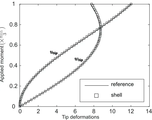
0 2 4 6 8 10 12 14

0 0.2 0.4 0.6 0.8 1

reference shell

Tip deformations

Applied moment

Figure 5: Load deflection curves for a cantilever shell subjected to an end moment

4 CONCLUSIONS

The analyses comfirm what has been known for many years, that shell elements can reduce the computational time significantly whilst still retaining the precision of hexahedra elements in bending cases. The compact MATLAB scripts given here provide engineers with a useful research tool to investigate the behaviour of shell structures. They are to be used in a coupled electro-mechanical analysis of a human heart as part of the first author’s PhD investigation. We are greatly indebted to Dr William Coombs of Durham University for providing us with his geometrically linear shell element code. This formed a crucial starting point for the development of the Total-Lagrangian analysis.

REFERENCES

[2] Coombs, W.M. et al. 70-line 3D Finite Deformation Elastoplastic Finite-element Code.Numerical Methods in Geotechnical Engineering : Pro. of the Seventh European Conference on Num. Met. in Geo. Eng. London: Taylor & Francis (2010) 151–156.

[3] European Heart Network.European Cardiovascular Disease Statistics (2017).

[4] Ruth, A.S.Electro-Mechanical Large Scale Computational Models of the Ventricular Myocarduium PhD thesis, Universitat Polit`ecnica de Catalunya (2004).

[5] Antonioletti, M.et al. BeatBox-HPC Simulation Environment for Biophysically and Anatomically Realistic Cardiac Electrophysiology. PLOS ONE (2017), 12(5).

[6] Ten-Tusscher, K.H. et al. A Model for Human Ventricular Tissue. Am. J. Physiol. Heart Circ. Physiol. (2004)286(4): H1573–H1589.

[7] Iyer, V. et al. A Computational Model of the Human Left-Ventricular Epicardial Myocyte. Biophys. J.(2004) 87(3): 1507–1525.

[8] Bueno-Orovio, A. et al. Minimal Model for Human Ventricular Action Potentials in Tissue. J. Theor. Biol. (2008)253(3): 544–560.

[9] Vigmond, E.J.et al. Computational Tools for Modeling Electrical Activity in Cardiac Tissue. J. Electrocardiol.(2003) 36(Suppl): 69–74.

[10] Pitt-Francis, J. et al. Chaste: Using Agile Programming Techniques to Develop Computational Biology Software. Philos. Trans. A. Math. Phys. Eng. Sci. (2008) 366(1878): 3111-3136.

[11] Clerx, M. et al. Myokit: A Simple Interface to Cardiac Cellular Electrophysiol-ogy.Prog. Biophys. Mol. Biol. (2016)120(1-3): 100–114.

[12] Okada, J.I. et al. Absence of Rapid Propagation through the Purkinje Network as a Potential Cause of Line Block in the Human Heart with Left Bundle Branch Block.

Front PHysiol. (2018) 9: 56.

[13] Bathe, K.J. and Bolourchi S. A Geometric and Material Nonlinear Plate and Shell Element. Comp. & Struc. (1980) 11: 23–48.

[14] Bathe, K.J. Finite Element Procedures. 2nd Edition, 2014.

[15] Bathe, K.J.et al. Finite Element Formulations for Large Deformation Dynamic Anal-ysis Int. Jour. for Num. Meth. In Eng.(1975) 9: 353–386.

[16] Stegmann, J. Finite Elements for Geometric Non-Linear Analysis Of Composite Laminates and Sandwich Structures. MSc thesis, Aalborg University (2001).