City, University of London Institutional Repository
Citation
:
Turkay, C., Slingsby, A., Lahtinen, K., Butt, S. and Dykes, J. (2017). Supporting
Theoretically-grounded Model Building in the Social Sciences through Interactive
Visualisation. Neurocomputing, 268, pp. 153-163. doi: 10.1016/j.neucom.2016.11.087
This is the accepted version of the paper.
This version of the publication may differ from the final published
version.
Permanent repository link:
http://openaccess.city.ac.uk/16153/
Link to published version
:
http://dx.doi.org/10.1016/j.neucom.2016.11.087
Copyright and reuse:
City Research Online aims to make research
outputs of City, University of London available to a wider audience.
Copyright and Moral Rights remain with the author(s) and/or copyright
holders. URLs from City Research Online may be freely distributed and
linked to.
Supporting Theoretically-grounded Model Building
in the Social Sciences through Interactive Visualisation
Cagatay Turkaya,∗, Aidan Slingsbya, Kaisa Lahtinenb,c, Sarah Buttb, Jason Dykesa
agiCentre, Department of Computer Science, City University London, UK bCentre for Comparative Social Surveys, City University London, UK cDepartment of Geography and Planning, University of Liverpool, UK
Abstract
The primary purpose for which statistical models are employed in the social sciences is to understand and explain phenomena occurring in the world around us. In order to be scientifically valid and actionable, the construction of such models need to be strongly informed by theory. To accomplish this, there is a need for methodologies that can enable scientists to utilise their domain knowledge effectively even in the absence of strong a priori hypotheses or whilst dealing with complex datasets containing hundreds of variables and leading to large numbers of potential models. In this paper, we describe enhanced model building processes in which we use interactive visualisations as the underlying mechanism to facilitate the construction and documentation of theory-driven models. We report our observations from a collaborative project involving social and computer scientists, and identify key roles for visualisation to support model building within the context of social science. We describe a suite of techniques to facilitate the exploration of statistical summaries of input variables, to compare the quality of alternative models, and to keep track of the model-building process. We demonstrate how these techniques operate in coordination to allow social scientists to efficiently generate models that are tightly underpinned by domain specific theory.
Keywords: visualization, visual analytics, model building, social science
1. Introduction
Scientists generally build statistical models for one of two main reasons; prediction and/or explanation. Within the social sciences, statistical models are almost exclu-sively used for explanation and to better understand the world around us and the underlying causal mechanisms driving human behaviour and/or attitudes. Such under-standing is necessary in order to affect change and improve society, for example, through policy interventions.
Commonly, statistical modelling in the social sciences is done using observed data (often from social surveys) and regression analyses to test a priori theoretically-derived causal hypotheses about the relationship between a set of explanatory variables, x, and an outcome, y. This involves a researcher-led process of defining theoretical constructs, deriving variables to measure these underlying constructs, running statistical models including these observed vari-ables, evaluating model results based on effect sizes and goodness of fit statistics, leading to conclusions and/or model refinement and retesting [1].
In the absence of well-defined theory and/or in the presence of large, new or complex data sets containing mul-tiple variables which cannot easily be reduced to a series of
∗Corresponding author
Email address: [email protected](Cagatay Turkay)
testable hypotheses, such an approach to statistical mod-elling may not always be feasible however. Social scientists may turn to prediction via data mining or machine learn-ing techniques in order to better understand the phenom-ena of interest [2]. Such an approach is likely to become increasingly common as social scientists move beyond a traditional reliance on social survey data as the basis of statistical modelling and embrace new forms of data [3]. The primary objective of such models nevertheless remains explanation; evidence from predictive modelling should be used to refine the underlying theory and develop hypothe-ses for subsequent testing. The relationship between ob-served data and underlying theoretical constructs there-fore remains of fundamental importance. If they are to be of use, it must be possible to relate the results of data-driven models back to sociological theory and the domain knowledge held by researchers and policy makers.
of the field of visual analytics – has already shown great potential [4, 5, 6] and our work contributes to this body of methods. In this paper, we describe our collaborative study in which we have designed and implemented inter-active visualisation techniques that enhance an existing workflow for constructing models. We introduce a number of techniques to: (a) assist in exploring statistical sum-maries of hundreds of variables, (b) facilitate comparison between the alternative models that are iteratively built and (c) help keep track of the modelling process and de-cision made. We describe and discuss our initial ideas on designs and functionalities. While developing these tech-niques, we derive general roles for visualisation in support-ing such involved model-buildsupport-ing processes and use these roles as guidance to inform our designs.
2. Related Work
The field of visual analytics [4, 7, 8] investigates how the merger of cognitive and creative capabilities of humans and computational power of algorithms advance the under-standing one can generate within data-intensive analysis cases. Within the context of numerical/statistical mod-elling, there are several examples where visual analytics has been applied successfully. Sedlmair et al. [5] gener-alise a subset of these work and present a framework for visual parameter analysis where they describe an elabo-rate data flow stelabo-rategy and suggest stelabo-rategies to navigate in the space of parameters with the guidance from visu-alisation. Afzal et al. [9] use a combination of interactive spatio-temporal visualisations and a decision history rep-resentation to support epidemiology model building. In their work, visualisation is a critical element to compare and evaluate different models and responses given to them. In Vismon [10], the authors designed a visualisation system to aid fishery managers to better model and better under-stand the uncertainties in the data and the computations. Torsney-Weir et al. [11] suggest a systematic parameter investigation process through visualisation in order to im-prove image segmentation models.
Visualization plays key roles in validating predictive models through interaction in the work by Piringer et al. [12]. The authors observed that a visualization-powered approach not only speeds up model building process but also increases the trust and confidence in the results. M¨uhlbacher and Piringer [13] discuss how the process of building re-gression models can benefit from integrating domain knowl-edge. Berger et al. [14] introduce an interactive approach to inspect the parameter space in comparison to multiple target values. Malik et al. [15] describe a framework that facilitates the interactive execution of auto-correlation meth-ods. Steed et al. [16] describe a visual analytics methodol-ogy where statistical regression, correlation analysis, and descriptive statistical calculations are incorporated as vi-sual guidance within an interactive system that enables the identification of important variables that can act as
significant predictors. They present their approach within the modelling of hurricane activity.
There are also methods that support feature selection tasks through visualisation. Krause et al.’s method [17] visually represents several cross-validation runs and gives an indication of how important particular features are for classification purposes. The authors observed that involv-ing the user in the model buildinvolv-ing process leads to eas-ier to interpret models. Interactive visual representations have been used to enhance the interpretation of decision trees [18] and clustering algorithm results [19].
Interactive systems have also demonstrated capabil-ity in improving the interpretabilcapabil-ity and explainabilcapabil-ity of computational models. Gleicher [20] describe Explainers – analyst crafted projection functions – that can explain the relations between the variables and the projection models more effectively. He describes how such expert generated models increase overall understanding of high-dimensional phenomena. Turkay et al. [21] demonstrate how visual in-teraction methods can be used to identify and represent local structures in high-dimensional spaces. Stahnke et al. [22] present an interactive method to modify the pa-rameters of a multi-dimensional scaling projection where accompanying visualizations display the contributions of the dimensions to the resulting clusters produced.
With our work, we advance the existing literature by emphasizing the importance of and suggesting new tech-niques for incorporate theory in the process of model build-ing. We also describe a set of roles for visualisation and demonstrate how geographical variation can be accounted for in model building processes.
3. Case study: European Social Survey (ESS)
In this paper, we carried out our investigations in the context of model building within the social science do-main and we draw observations, identify needs, and of-fer solutions from our work with social scientists involved with the European Social Survey (ESS). The ESS is an academically driven, methodologically rigorous survey of public attitudes and opinion which has been carried out in around 25 countries every two years since 20011. Data
covering a variety of social, political and demographic top-ics are collected from a nationally representative sample of the population in each country and used to conduct a wide range of substantive and methodological analyses. The particular focus of the ESS research used as a case-study for this project was to better understand why people do or not participate in the survey i.e. to model survey non-response. However, as will be discussed further in the concluding sections, the goals, data and methods employed in this research - and hence observations based on how in-teractive visualisation may be employed - are increasingly
Model building
1. Build modelUse informed subset
2. Quantify its fitness
Coefficients, ANOVA, R2,
p-values, cross validation
3. Populational &
Geographical variation 4. Keep a record of
alternatives and fitness 5. Annotate models
Variable selec
ti
on and understanding
Social theory
Theory that justifies the variable’s use
e.g. deprivation, crime, anti-social behaviour, quality of life
Single variables
Characteristics of variables
Descriptive statistics
Rela
ti
onship between variables
Similarity between variables
Co-variance, MDS, Correlation with targets
1.
Understand variables be
tt
er by
whi
tt
ling down to manageable
number
2.
Itera
ti
vely build
models based on
fi
tness of previous
3.
Final
model
~400 variables
~40 variables
R1
R2
R2
R3
R4
R6
R7
[image:4.595.100.495.83.331.2]R8 R5
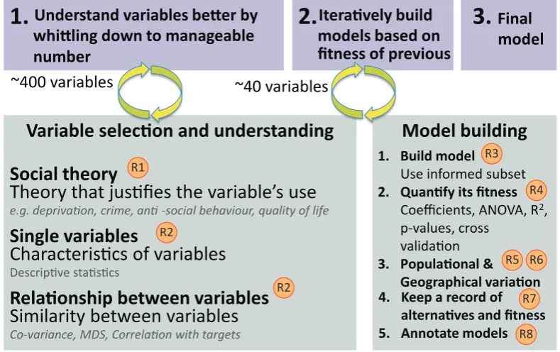
Figure 1: An illustration to summarise the enhanced model-building process and the key roles we identified for interactive visualisation to enhance this as described in Section 3.2 (labelledRn). The process moves between variable selection and model-building, and our techniques facilitate an iterative model-building process.
applicable to model building in other areas of the social sciences.
As part of the ESRC-funded ADDResponse project2 ESS researchers were interested in using auxiliary data to better understand individuals propensity to respond to social surveys. There is considerable interest in be-ing able to both predict and understand individuals re-sponse decisions so that researchers can intervene to im-prove response rates, especially among typically hard to reach groups who may otherwise be underrepresented in the final dataset [23]. Despite a large and growing field of research, and relatively well-developed theoretical mod-els, social scientists have had relatively little success in modelling response behaviour empirically [24]. One pos-sible explanation for this may be a lack of suitable data available with which to model the behaviour of both re-spondents and nonrere-spondents (for whom, by definition, survey data are not available) and to test underlying theo-ries. In order to address this possibility, ADDResponse appended auxiliary data from a variety of external sources -small-area statistics from administrative sources, commer-cial consumer profiling data and open source data about their physical location - to the geographically structured sample of 4,520 addresses selected to take part in Round 6 of the ESS in the UK 2012-13 and conducted extensive analysis of survey nonresponse.
The wealth of auxiliary variables (401 variables from 20 different sources) available for analysis represents both
2www.addresponse.org
the strength of the ADDResponse project and a signifi-cant challenge for researchers. Researchers were faced with a multitude of unfamiliar variables from external sources which, unlike the survey data themselves, were not col-lected specifically for the purpose of research and so were not theoretically constructed. This requires a different way of thinking about the data and the modelling process than would usually be the case. Social scientists explor-ing survey non-response typically start with a finite set of theoretically-defined constructs, design or select vari-ables to measure these constructs, and then run a pre-determined set of models to test hypothesised associations between these designed variables [25, 26]. Even where machine-learning techniques such as regression trees have been used to study nonresponse, there has usually been careful pre-selection of variables on theoretical grounds to make the analysis manageable [27]. In contrast, the ADDResponse project started with a range of variables at its disposal andthen faced the need to organise these variables around theoretical constructs, make selections between these variables for modelling purposes and then choose between alternative models. Our approach to or-ganising the variables is to identify a set ofsocial theories
con-cepts are associated with social science theories.
In order to provide more than statistical prediction and derive models which could ultimately be interpreted and used by survey practitioners, researchers still need to be able to ground their variable selection and model build-ing in theory and relate it back to expert domain knowl-edge. However, with so many unknown and potentially overlapping and/or redundant auxiliary variables, and sev-eral possible theoretical hierarchies (theories → concepts
→variables), this is not a straightforward process and in-volves variety and uncertainty at all steps of the process. It does, however, make the ADDResponse project an ideal case study for exploring how interactive visualization could help to inform and streamline this process.
Computer and social scientists collaborated closely through-out the project and, from the start, the tool has been de-signed around the needs of the intended end-users. There were frequent discussions between researchers across the two disciplines to map out workflows, specify tool require-ments and explore the potential capabilities afforded by visualisation. Discussions were backed up by observation sessions in which the computer scientists observed the so-cial scientists at work using their existing pre-visualisation tools and workflows and interactive sessions in which com-puter scientists demonstrated the prototype tools using the ADDResponse dataset and answered questions and received feedback from the social scientists. During the main tool development period weekly meetings between researchers provided an efficient way for new features to be demonstrated to the intended end-users, receive feed-back and be improved upon.
3.1. Existing model building workflow
Social researchers working on a project such as AD-DResponse, the goal of which is to model observed data using regression analysis to better understand associations (and ultimately causal links) between variables, face a number of tasks and decisions. These include: under-standing the distributions and underlying properties of the data, variable selection, model selection and compu-tation, and evaluating effect sizes and model fit. Model building is often an iterative process with models rede-fined and variables included or excluded from subsequent models based on prior results. Frequently, multiple models will need to be considered alongside one another, explor-ing different outcome variables and/or comparexplor-ing patterns across different populations. Given the end goal of expla-nation, the ability to relate decisions and results back to sociological theory and domain knowledge remains impor-tant throughout the process. Researchers rely on a variety of statistical and graphical tools to inform their decision making process. For example, scatter plots, histograms or other graphical representations of variables may be pro-duced to better understand the underlying data. Data reduction techniques such as principal components anal-ysis may be applied to assist in variable selection, iden-tifying and grouping observed variables which are
mani-festations of the same underlying concept [28]. Different regression techniques may be used to model associations between variables depending, for example, on the nature of the data (e.g. logistic regression for binary outcome vari-ables), what is assumed about the relationship between the outcome and predictor variables, and the desired degree of automation in model selection [29]. Model results are reviewed alongside regression diagnostics to check for po-tentially problematic variables (e.g. outliers, homoscedas-ticity or overlapping variables) and a range of goodness of fit measures are available to assist in evaluating the suc-cess of the model in explaining the outcome variable of interest [30]. Often used measures are Akaike Information Criterion (AIC) and McFadden Pseudo-R2[31]. AIC is an information theoretical measure to estimate the informa-tion loss in models where analysts can select the one with the least loss (i.e., smallest score) among several competing models [32]. Whereas McFadden is one of the pseudo-R2
measures to estimate model fit and get values within the [0,1] interval [31]. Software packages such as STATA or R facilitate increasingly varied and complex statistical analy-sis as well as incorporating sophisticated graphics packages for visualising both the underlying data and results. Syn-tax and output files can be annotated and used to keep track of outputs produced and decisions made.
A significant limitation of existing software and the approach to model building that it supports is that it is predominantly based around the idea of researchers speci-fying and running distinct analyses as part of a sequential, linear process. The results of these analyses are then dis-played separately from both previous/subsequent analyses and any available metadata e.g. information on the source or theoretical rationale behind the variables. Where the re-searcher is equipped with a limited number of pre-defined and theoretically grounded variables and models (as has often been the case among social scientists in the past), this need not be a problem. However, as researchers face the challenge of making sense of increasingly complex and unfamiliar datasets and produce multiple, iterative models whilst attempting to relate the results back to underlying theory, a straightforward linear cataloguing of inputs and outputs is likely to prove insufficient and a more holistic and dynamic approach is required. At the start of the ADDResponse project, researchers used a combination of excel spreadsheets, Post-it notes arranged and rearranged on the office wall and written notes to try and keep track of the analytic process and make comparisons across the-ories, variables and models. Interactive visualisation has the potential to provide a more streamlined solution.
3.2. Key roles for interactive visualisation
A
B C
Sel.2 : Deprivation Sel.1 : High Skew
D
E
[image:6.595.66.532.81.358.2]F
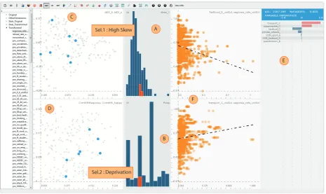
Figure 2: VarXplorerhelps to visually explore the variables and items concurrently – scatterplots with blue dots (C, D) visualise the variables where those with orange ones involve items (F). Interactive model building is also incorporated and computations are triggered in response to user selections (E). Here a series of selections of subsets of variables are made and the resulting models are inspected as explained in Section 4.1.
as key guiding principles to inform our designs and tech-niques we develop in this paper. We annotate them asRn
and refer to these roles wherever appropriate in the later sections.
3.2.1. Incorporating Theory
R1: Provide interactive access to theoretical annotations.
Variables’ potential suitabilities for building models need to be informed by social science theory (i.e., how strongly they relate to the theories & concepts as explained above). One way to incorporate such knowledge is to externalise the relations between the variables, concepts, and the theo-ries, and make these accessible as interaction points through-out the process. One possible way to do this is to encode such knowledge as metadata about the variables and mak-ing that data available for selections throughout the inter-active analysis.
3.2.2. Exploring variables
R2: Provide on-demand statistical and graphical summaries of variables, comparisons and relationships to each other.
Variables’ potential suitabilities are also informed by their statistical and geographical distributions and correlations with each other. During the process, analysts need to explore, investigate and compare variables on-demand to maintain a multi-perspective understanding.
3.2.3. Interactively building models
R3: Real-time computation of models on interactively de-fined domains. Due to the multidimensional and open-to-interpretation nature of phenomena being modelled, meth-ods to easily trigger model computations with interactively defined domains are needed to flexibility compare and con-trast several alternatives. Computational models need to run seamlessly in response to users’ interactive inputs with results being communicated through appropriate visual representations.
R4: Immediate feedback on model success. Such interac-tive model building should also be informed by different metrics of model fitness and success so that the analysts can make judgments easily and efficiently. The users need to receive an immediate response on whether an interactive action has improved the predictive power of the model.
3.2.4. Considering different populations
R5: Compare models and statistics across populations.
comparing the properties of variables and/or model re-sults across these different populations and grouping and tracking outputs by population.
R6: Provide geographically constrained models and statis-tics. Geographical aspects of these response models are important and the drivers of non-response bias are likely to vary geographically, thus requires special consideration. In contrast to conventional models, such geographically constrained results provide insight into the “locality” of the models. In contrast to the global models, however, such an approach involves several local models that need to be considered and compared. This calls for effective visualisation methods where the quality of all these local models can be inspected within their geographical context.
3.2.5. Recording the model-building process, i.e., prove-nance
R7: Maintain history of model building steps. One critical expectation during iterative model building processes is to be able to document the different models built, compare the variables they contain and their performance (often referred to as provenance [33]). This is in particular im-portant in presenting and defending the decisions made during the modelling iterations and explain how the pro-cess converged towards a set of plausible models.
R8: Allow models to be annotated. As also highlighted in the above discussion, the scientists need to reflect back on their process and explain why a variable is kept or dis-carded from the model. This is often best accomplished through annotations and notes to document the decisions made. Thus, there is a need to offer facilities to annotate models with notes to help researchers recall their decisions.
4. Enhancing the workflow
Fig. 1 shows how we are augmenting the existing pro-cess. In this work, we have done so with separate tech-niques that we realized through disjoint prototypes in or-der to test the methods themselves. Using an established approach involving user-centred iterative prototyping/feed-back cycles [34, 35], we designed interactive visualisation to meet these requirements as three prototypes. Our de-signs are informed by established advice as to effective ways of mapping visual variables to data variables [36, 37]. We initiated our process with the incorporation of the methods that are in use within the existing model build-ing process (as described above), namely the logistic re-gression as the modelling tool and the AIC and McFad-den measures for assessing the model fit. In addition to these techniques, we also investigated the incorporation of a purely data-driven perspective and also fed the data into a random forest classifier [38] implementation3 and investigated whether the variable importance values are in agreement with those identified through other methods.
3http://scikit-learn.org
Our decision here to utilise random forest technique is in-formed by evidence in the social science literature that ensemble methods carry the potential for additional roles on top of the more common classification and forecast-ing roles, namely, servforecast-ing as diagnostics tools to conven-tional methods, and providing further insight into the rela-tion between the explanatory and response variables [39]. Moreover, their conceptual resemblance to wider adopted methods such as regression trees [27], make them a suit-able candidate to introduce as a data-driven methodology into the process.
4.1. VarXplorer: exploring statistical relations between vari-ables
The first prototype we designed and developed for this use-case is the interactive multiple coordinated view envi-ronment we refer to as VarXplorer. Fig. 2 shows VarX-plorer designed to meet requirements related to under-standing the input variables and how they relate to each other (R1 & R2) and also includes model building and immediate feedback (R3 & R4) with geographical con-siderations (R6). Here we employ multiple visualisations where several selections made through each can be com-bined using Boolean operations. The users have the flexi-bility to select any of the variables and/or meta-data (se-lecting from the left-most pane in Fig. 2) and utilise an appropriate visualisation.
In order to have the variables as our main visual en-tities in the graphics, we employ a technique called dual-analysis [40]. To enable this, for each variable we compute several general and domain-specific measures and projec-tions: i) Statistical moments such as (sample) mean (µ), (sample) variance (σ), skewness, kurtosis etc. ii) correla-tions with response outcome and other key variables such as happiness score, social trust, etc. iii) multidimensional scaling (MDS) on the variables where the distance is pair-wise correlations (in a similar fashion to Turkay et al. [21]) iv) metadata that externalise the concepts/theories vari-ables relate to (R1). Variables are visualised over different measures that characterise them, e.g., a scatterplot where one axis isσof the variables and the other is the correla-tion with the average response rate in an area (postcode sector) and each dot is a variable. In addition to these variable visualisations, VarXplorer also supports visuali-sations where the main visual elements are the data items (4520 survey participants in this case). In order to support the distinction between these two types of views, variable plots have blue dots to indicate a single variable and items plots have orange dots.
In addition to the interactive visualisations, a number of computational tools have been integrated in the system to respond to interactions from users. Given that we aim to generate models to estimate non-response within this work, we incorporate logistic regression where the target
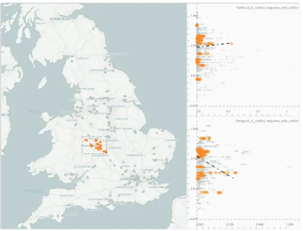
Figure 3: Interactively setting a geographical focus around the West Midlands region and observing the relation between response rate and the two variables (as identified in Fig. 2) “locally” for the selected region. Notice how both the relations changed “sign” compared to their “global” counterparts.
of variables, the logistic regression computations are trig-gered instantly operating “only” on the selected variables. A visual representation of variable weights is generated automatically to indicate the importance of variables (or-dered red or blue bars as seen in Fig. 2F). We decided to use the length of the bars to indicate the importance of variables since length is a visual variable that works well, in particular when ordered for comparison [37, 36]. We also support the length with two different colors to indicate the sign of the weight. In a similar fashion, we also incorporated a linear-regression method working in conjunction with scatterplots, again operating only on the selected items (see the two plots in Fig. 2F) (R5).
In Fig. 2, we start with a selection of highly skewed variables (with the assumption that they might carry dis-tinctive characteristics) with a selection through a his-togram of variables’ skewness values (Fig. 2A). This is followed by a selection (with an AND operation) on the variables intended to provide measures of (or proxies for)
deprivation one important theorised driver of survey non-response [25]. Again through a histogram of variable meta-data (Fig. 2B). The MDS of variables (Fig. 2C) reveals variability in the set of resulting variables (i.e., not all of them are inter-correlated), thus provide a plausible set to run a model locally. A logistic regression model is com-puted in real-time on this selection of variables. The vi-sual representation of variables’ importance (Fig. 2E) indi-cate thataccess to public transport,access to supermarkets
and count of fast food outlets as having higher weights in this model. However, goodness of fit metrics appropriate to models used for binary dependent variables (AIC and
McFadden pseudo-R2) signal low predictive strength, i.e.,
0.023 for McFadden R2 (possible range 0-1), (Fig. 2C blue bar) [41]. To evaluate the variables further, we pulled up two scatterplots where y-axes are the average response rate in the local area and x-axes areaccess to fast food and ac-cess to public transportrespectively (Fig. 2F). Notice that the former is negatively and the latter is positively cor-related with response rates. Other characteristics of the variables are investigated through a plot ofcorr. with re-sponse andcorr. with happiness (Fig. 2D).
We also support the investigation of geographical vari-ation (R6) in the computed results. In Fig. 3, we keep the two scatterplots from the previous setting, but this time trigger “local” regression computations for the West Midlands region in the UK. We observe that both of the correlation relations changed sign for this area, possibly indicative of the different social structures in the region.
4.2. VarMaps: exploring the geographical distribution of variables
The UK ESS4sample is geographically clustered in or-der to achieve a nationally representative sample of the population whilst making it cost-effective to carry out face-to-face data collection. At the first stage, a sample of 226 Primary Sampling Units (postcode sectors) was drawn. Twenty addresses were then sampled within each Primary Sampling Unity (PSU) to achieve a final sample of 4,520 addresses. The resulting geography is 226 sets of geograph-ically tight clusters of locations (Fig. 4, left). Our novel
Figure 4: The 226 sets of 20 tightly clustered household locations (left) required novel cartographic design (right) to present the data in a non-occluding manner that preserves the two-level hierarchy and retains much of its geographical distribution. The middle image is an intermediate step in the transformation to illustrate how the two maps relate to each other [42]. This shows the geographical pattern of how people responded to the ESS survey at two geographical scales: by household and by Primary Sampling Unit.
cartogram-like layout [42] in (Fig. 4, right) spreads these out so that none overlap, revealing the 226 sets of tightly-clustered household locations, retaining much of the geo-graphical distribution. When used with population vari-ables such as Fig. 7, it allowed our users to consider the geographical distribution of two geographical scales simul-taneously – local volatility in values (within few streets) and wider geographical patterns – in a non-occluding man-ner (R6). Since the data in our case study are inher-ently spatial, this prototype allow modelling decisions to be made according to the geographical distribution of the variables. The following sections contain examples on how these maps inform the variable selection and model build-ing decisions.
4.3. ModelBuilder: supporting, evaluating and recording the model-building process
Fig. 5 shows theModelBuilder prototype designed to meet the requirements related to building models including the incorporation of theory and expert knowledge (R1), interactively-building models (R3) with detail of fit (R4) and models that are fit to all 11 geographical regions (R6), maintain-ing a history of models built (R7) and allowing annota-tions to be attached to the models (R8).
For a given outcome variable and starting with an empty model root (Fig. 5D), clicking on potential explanatory variables (one of the variables listed in Fig. 5B) creates a new model that adds the variable to the set of variables in the model. As the user adds variables to the model, the model tree develops to show the provenance of the process (Fig. 5D). The variable’s contribution to the se-lected model (highlighted in yellow in Fig. 5E) is shown for each explanatory variable (brown to green in Fig. 5C) and a measure of overall model fit (AIC) is shown for each
model (red in Fig. 5E). This history is shown as a tree structure (R7), recording the process through which the analyst constructed the model, allowing models to be com-pared. Free text annotation (R8) allows decisions to be recorded, and a red cross indicates where the analyst con-siders the iterative process to have reached a dead-end. A separate model is built for each of the 11 geographical regions (R6), laid out geographically in a grid-map [43] according to Fig. 5F. This layout depicts both the contri-bution that the variable makes to the model (Fig. 5B) and the model fit (Fig. 5E).
4.4. The Model Building Process
Here we walk through our suggested model building process that involves the use of the techniques introduced in the previous section. The scientists initiate their analy-sis by investigating the relationships between the variables together with their associations with the known social sci-ence theory concepts inVarXplorer. This process ends up with a selection of variables which then can be investi-gated for spatial variation through VarMaps and used as a starting point in building a model to predict survey non-response throughModelBuilder. ModelBuilder acts as the interactive mechanism to improve the model in a step-wise fashion and keep a record of this process.
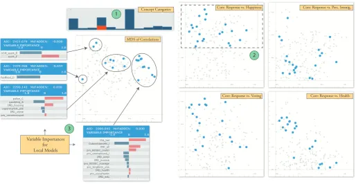
We start our investigation of the variables by looking into the concepts with which they are associated. Our strategy here is to focus on a number of concepts and aim to choose effective proxy variables for these. Fig. 6 exemplifies an explorative session where we begin with selecting the variables that can be proxies for “depriva-tion” (Fig. 6A). Looking at the four variable correlation maps (right, where x-axes are always correlation with the
B
C
E A
[image:10.595.91.505.81.248.2]D F
Figure 5: ModelBuilder. Prototype that implements the model building workflow for an outcome variable, in this caseresponse outcome
(highlighted text in red). The candidate variables to go into the model are listed (B) and the user can interactively generate a series of models building a tree to indicate the model-building provenance (D). The model fit is computed both globally and locally for various geographical regions and communicated through appropriate color mappings. Further details are in Section 4.3.
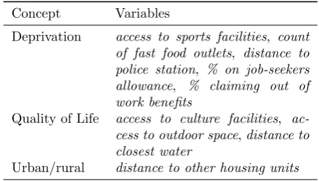
ESS indicators), we notice different correlation relations with the different ESS indicators and limit our attention to those that correlate with high levels of reported hap-piness (Fig. 6B). The MDS plots reveals sets of variables that are correlated within each other. We locally apply logistic regression on these subsets (Fig. 6C) and choose one or two representative from each of these sub-groups. A similar process is applied to other concepts such as “qual-ity of life” and “urban/rural life”, leading to a total of 9 variables. These variables are listed in Table 1. At this stage, we decided to include one more variable, electricity consumption, which was suggested by the random forest algorithm as one of the most discriminating variables to estimate response outcome.
We extend this list with a short list of variables that are thought to be important to include in the model to ex-plain non-response as informed by existing literature [25]:
% flats in an area, and ethnic fractionlisation, and select those manually in VarXplorer (not shown in images). The histogram of concept types revealed that these variables relate to individual characteristics and heterogeneity as the theoretical concepts.
We then move on to investigating the geographical vari-ations of these variables and observe theVarMaps for the selected variables. Fig. 7 lists the VarMaps for count of fast food outlets, access to outdoor space, and % on job-seekers allowance. Notice the London dominance for the
count of fast food outlets variable whereas the distribution of access to outdoor space is more even – making the lat-ter more suitable to include in “global” models. The same can be told forelectricity consumption which is identified as important by the random forest classifier which is run globally in this instance.
These variables are then selected inModelBuilder one by one for a more thorough, manual model building ses-sion. We build several models with different combinations.
Table 1: List of variables chosen in Section 4.4 and the associated concepts
Concept Variables
Deprivation access to sports facilities, count of fast food outlets, distance to police station, % on job-seekers allowance, % claiming out of work benefits
Quality of Life access to culture facilities, ac-cess to outdoor space,distance to closest water
Urban/rural distance to other housing units
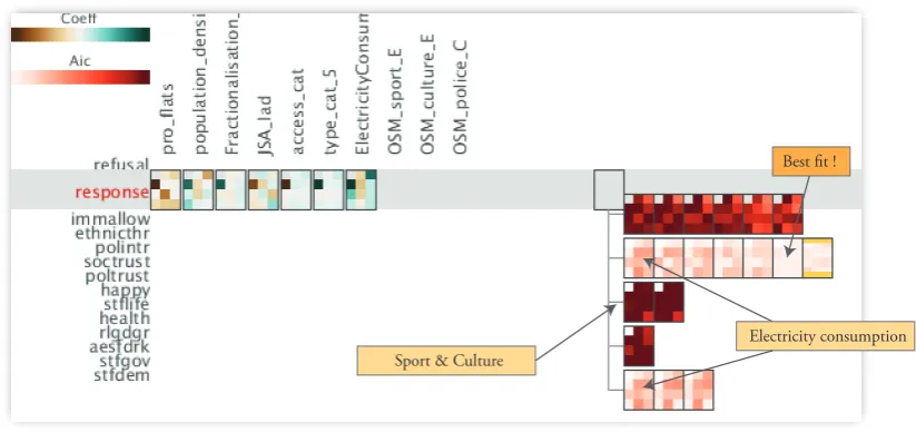
Investigating the variables’ contributions to the model fit, we observed that electricity consumption is the one that improves the model fit by far the best. This can be ex-plained by the even distribution of its values. The other variables, however, are often geographically varied, hinder-ing their contribution to the overall model fit. The model that fits the best is not only globally a good fit but also highly persistent locally, i.e., low variation within the 11 regions – indicating further the suitability of the model to act as an effective global model. One observation here is that we were able to generate several models to visually inspect all of these concurrently through our technique.
4.5. Reflecting on the enhanced model building process
[image:10.595.315.548.350.482.2]Corr: Response vs. Perc. Immig.
Corr: Response vs. Health Corr: Response vs. Voting
MDS of Correlations Concept Categories
Variable Importances for Local Models
1
2
Corr: Response vs. Happiness
[image:11.595.42.557.81.347.2]3
Figure 6: An example interactive variable selection process. After a series of filtering the variable set (A,B), logistic regression is computed locally for the observed sub-structures in the MDS plot (C). The four variable importance distributions indicate the characteristics of the different models built. Further details in Section 4.4
means that the resulting models are easier to defend, ex-plain, and use as the basis for action.
In the following, we reflect back on the five key role categories we have identified in Section 3.2 and discuss the ways that the visualisation enhanced model-building approach has affected the process. Notice that these are observations made (by the social scientist authors) during the modelling sessions carried out as a team of computer and social scientists as described in Section 3.
Incorporating Theory - Having access to metadata and being able to select variables on the basis of what they are proxies for and then to run analysis on each the-oretically linked group was useful in helping to build and track theoretically grounded models even whilst data min-ing/exploring unfamiliar variables.
Exploring variables - Being able to plot and compare properties of variables as well as cases was helpful espe-cially when used alongside mapping and metadata func-tions. This was particularly helpful to identify possible outlier variables which are either highly geographically skewed variables, or variables which had been assumed as proxies for a particular construct, e.g. deprivation, but appeared unrelated to others in the same domain empiri-cally.
Interactively building models - Being able to click to select/unselect variables and observing the colour coded fit statistics/parameter estimates made it very efficient to run and get an overview of different models and to compare the marginal effect of adding/excluding particular variables.
Considering different populations - Being able to de-fine and flexibly alter the definitions of “interesting” sub-sets is a powerful capability. Having access to all the dif-ferent data facets of survey responses, such as geographical location or demographics, and interactively defining mul-tiple sub-populations and comparing their impacts on the produced models is an important enhancement through visualisation.
Recording the model-building process - Being able to keep track of previous models and which variables had/hadn’t been included was particularly useful. This is a process which is otherwise quite hard to do, i.e., the use of post it notes and textual output with annotations.
5. Discussions, limitations and further work
In this paper, we realized our techniques through dis-joint prototypes rather than focussing on a single com-bined tool. Wherever needed, we manually established the information transfer between them, e.g., selecting a set of variables from VarXplorer and iteratively include them in models built in ModelBuilder. We think this is less disruptive to the modelling-building process and im-proves adoption.
Figure 7: Left to right:VarMapsforcount of fast food outlets,access to outdoor space,% on job-seekers allowance, andelectricity consumption. Notice the London dominance for thecount of fast food outletswhereasaccess to outdoor spaceis in general evenly distributed.
without compromising the social scientists’ expert knowl-edge so that greater confidence in the models is achieved. It is important to mention that in this paper we have not followed a structured, formal evaluation study where the overall model building process is compared with and without the tools being introduced. We instead gathered qualitative feedback and documented observations during the joint analysis sessions and reported on the improve-ments in Section 4.5. This decision was mainly due to the fact that the existing model-building workflow (prior to the project) were not involving capabilities such as interactive visualisation enabled model building, model provenance or geographical variable maps, making a direct comparison not feasible. One can, however, adopt more formal eval-uation study strategies such as insight based evaleval-uation methods [44], to further validate separate processes within the methods suggested. We leave this to future work and in addition also plan to make further observations on be-havioral changes as the tools are further adopted.
In this paper, we consider model building for a partic-ular purpose and in a particpartic-ular context. Our focus is on social science models where the primary purpose is expla-nation and results and conclusions need to be grounded in sociological theory or domain knowledge. There has also been a particular focus on modelling involving large or unfamiliar datasets where the observed variables were not essentially collected for the purpose of the research study or underpinned by a pre-defined theoretical construct and where researchers may require additional tools to help them relate exploratory, data-driven analysis back to the-ory. It is important to recognise that not all modelling problems are of this sort. In the event that researchers have access to primary data comprising a small number of specifically-collected variables and are focused on test-ing pre-defined theoretically-driven hypotheses about as-sociations between variables (e.g. evaluating the effect of offering a £5 incentive to participate on survey response rates after running an experiment in which one group were offered no incentive and another, matched group, were of-fered a £5 incentive to complete the same survey)
inter-active visualisations may be unnecessary to support anal-ysis. Similarly, in the event that the primary goal is pre-diction of future behaviour on the basis of past behaviour e.g., within an online shop where purchasing records are collected to build a recommendation system, there is less room for involving a human expert and a purely data-driven methodology could be much more effective, consid-ering the cost of an interactive process in terms of human time.
Nevertheless, although the discussion and development is strongly rooted in a specific case study – that of ex-ploring nonresponse to the European Social Survey – the roles identified for interactive visualisation in this study have wide applicability across the social sciences. As the growth of big data and the move towards open data con-tinue, social scientists will increasingly turn to exploring the potential afforded by auxiliary data not collected with research in mind to understand as well as predict human attitudes and behaviour. As they do so, tools which aid researchers to explore unfamiliar variables, to construct, compare, interpret and record the provenance of multiple models, and to do this whilst maintaining the link between data and domain knowledge will become increasingly im-portant.
6. Conclusion
Electricity consumption Sport & Culture
[image:13.595.94.506.85.279.2]Best fit !
Figure 8: Model Builder to investigate several model alternatives based on the set of variables identified. Best fit models (lower AIC scores, palish colors) are those often involve the electricity consumption variable.
visualisations to support the kinds of model building pro-cesses we investigate in this work. We also demonstrate how disjoint “prototypes” can lead to effective analysis ses-sions without the need for laborious software engineering work.
Acknowledgments
This work is partly funded by ADDResponse project funded by the UK Economic and Social Research Council (grant ES/L013118/1).
References
[1] G. Shmueli, To explain or to predict?, Statistical Science 25 (3) (2010) 289–310.
[2] M. Hindman, Building better models prediction, replication, and machine learning in the social sciences, The ANNALS of the American Academy of Political and Social Science 659 (1) (2015) 48–62.
[3] V. Mayer-Sch¨onberger, K. Cukier, Big data: A revolution that will transform how we live, work, and think, Houghton Mifflin Harcourt, 2013.
[4] D. Keim, F. Mansmann, J. Schneidewind, J. Thomas,
H. Ziegler, Visual analytics: Scope and challenges, in: Visual Data Mining, Springer-Verlag, 2008, pp. 76–90.
[5] M. Sedlmair, C. Heinzl, S. Bruckner, H. Piringer, T. Moller, Vi-sual parameter space analysis: A conceptual framework, ViVi-sual- Visual-ization and Computer Graphics, IEEE Transactions on 20 (12) (2014) 2161–2170.
[6] C. Turkay, F. Jeanquartier, A. Holzinger, H. Hauser, On computationally-enhanced visual analysis of heterogeneous data and its application in biomedical informatics, in: Interactive Knowledge Discovery and Data Mining in Biomedical Informat-ics, Springer, 2014, pp. 117–140.
[7] D. Keim, J. Kohlhammer, G. Ellis, F. Mansmann, Mastering the information age solving problems with visual analytics. [8] J. J. Thomas, K. A. Cook, Illuminating the path: The research
and development agenda for visual analytics, IEEE Computer Society Press, 2005.
[9] S. Afzal, R. Maciejewski, D. S. Ebert, Visual analytics decision support environment for epidemic modeling and response eval-uation, in: Visual Analytics Science and Technology (VAST), 2011 IEEE Conference on, IEEE, 2011, pp. 191–200.
[10] M. Booshehrian, T. M¨oller, R. M. Peterman, T. Munzner, Vis-mon: Facilitating analysis of trade-offs, uncertainty, and sensi-tivity in fisheries management decision making, in: Computer Graphics Forum, Vol. 31, Wiley Online Library, 2012, pp. 1235– 1244.
[11] T. Torsney-Weir, A. Saad, T. Moller, H.-C. Hege, B. Weber, J.-M. Verbavatz, S. Bergner, Tuner: Principled parameter finding for image segmentation algorithms using visual response surface exploration, IEEE Transactions on Visualization and Computer Graphics 17 (12) (2011) 1892–1901.
[12] H. Piringer, W. Berger, J. Krasser, Hypermoval: Interactive visual validation of regression models for real-time simulation, in: Proceedings of the 12th Eurographics / IEEE - VGTC Con-ference on Visualization, EuroVis’10, Eurographics Association, Aire-la-Ville, Switzerland, Switzerland, 2010, pp. 983–992. [13] T. Muhlbacher, H. Piringer, A partition-based framework for
building and validating regression models, Visualization and Computer Graphics, IEEE Transactions on 19 (12) (2013) 1962– 1971.
[14] W. Berger, H. Piringer, P. Filzmoser, E. Gr¨oller, Uncertainty-aware exploration of continuous parameter spaces using mul-tivariate prediction, Computer Graphics Forum 30 (3) (2011) 911–920.
[15] A. Malik, R. Maciejewski, N. Elmqvist, Y. Jang, D. S. Ebert, W. Huang, A correlative analysis process in a visual analyt-ics environment, in: Visual Analytanalyt-ics Science and Technology (VAST), 2012 IEEE Conference on, IEEE, 2012, pp. 33–42. [16] C. A. Steed, J. E. Swan, T. Jankun-Kelly, P. J. Fitzpatrick,
Guided analysis of hurricane trends using statistical processes integrated with interactive parallel coordinates, in: Visual An-alytics Science and Technology, 2009. VAST 2009. IEEE Sym-posium on, IEEE, 2009, pp. 19–26.
[17] J. Krause, A. Perer, E. Bertini, Infuse: interactive feature selec-tion for predictive modeling of high dimensional data, Visual-ization and Computer Graphics, IEEE Transactions on 20 (12) (2014) 1614–1623.
2011, pp. 151–160.
[19] E. Kandogan, Just-in-time annotation of clusters, outliers, and trends in point-based data visualizations, in: Visual Analyt-ics Science and Technology (VAST), 2012 IEEE Conference on, IEEE, 2012, pp. 73–82.
[20] M. Gleicher, Explainers: Expert explorations with crafted projections, IEEE transactions on visualization and computer graphics 19 (12) (2013) 2042–2051.
[21] C. Turkay, A. Lundervold, A. J. Lundervold, H. Hauser, Rep-resentative factor generation for the interactive visual analysis of high-dimensional data, IEEE Transactions on Visualization and Computer Graphics 18 (12) (2012) 2621–2630.
[22] J. Stahnke, M. Dork, B. Muller, A. Thom, Probing projec-tions: Interaction techniques for interpreting arrangements and errors of dimensionality reductions, Visualization and Computer Graphics, IEEE Transactions on 22 (1) (2016) 629–638. [23] A. Peytchev, Consequences of survey nonresponse, The
AN-NALS of the American Academy of Political and Social Science 645 (1) (2013) 88–111.
[24] D. S. Massey, R. Tourangeau, Introduction: New challenges to social measurement, The ANNALS of the American Academy of Political and Social Science 645 (1) (2013) 6–22.
[25] R. Groves, M. Couper, Nonresponse in household interview sur-veys, John Wiley & Sons, 2012.
[26] J. Bethlehem, F. Cobben, B. Schouten, Handbook of nonre-sponse in household surveys, Vol. 568, John Wiley & Sons, 2011. [27] D. Toth, P. Phipps, Regression tree models for analyzing survey response, in: Proceedings of the Government Statistics Section, American Statistical Association, 2014, pp. 339–351.
[28] D. J. Bartholomew, F. Steele, J. Galbraith, I. Moustaki, Anal-ysis of multivariate social science data, CRC press, 2008. [29] G. James, D. Witten, T. Hastie, R. Tibshirani, An introduction
to statistical learning, Springer, 2013.
[30] J. S. Little, Goodness-of-fit measures, in: M. Lewis-Beck, A. Bryman, T. F. Liao (Eds.), The SAGE Encyclopedia of So-cial Science Research Methods, SAGE Publications, Inc., Thou-sand Oaks, 2004, pp. 436–437.
[31] K. P. Burnham, D. R. Anderson (Eds.), Model Selection and Multimodel Inference: A Practical Information-Theoretic Ap-proach, Springer Science+Business Media, 2004.
[32] K. P. Burnham, D. R. Anderson, Kullback-leibler information as a basis for strong inference in ecological studies, Wildlife research 28 (2) (2001) 111–119.
[33] E. Ragan, A. Endert, J. Sanyal, J. Chen, Characterizing prove-nance in visualization and data analysis: An organizational framework of provenance types and purposes, Visualization and Computer Graphics, IEEE Transactions on 22 (1) (2016) 31–40. [34] J. Gulliksen, B. G¨oransson, I. Boivie, S. Blomkvist, J. Persson,
˚
A. Cajander, Key principles for user-centred systems design, Behaviour and Information Technology 22 (6) (2003) 397–409. [35] J. Dykes, J. Wood, A. Slingsby, Rethinking map legends with vi-sualization, IEEE Transactions on Visualization and Computer Graphics 16 (6) (2010) 890 – 899.
[36] J. Bertin, Semiology of Graphics, University of Wisconsin Press, 1983.
[37] W. S. Cleveland, R. McGill, Graphical perception: Theory, ex-perimentation, and application to the development of graph-ical methods, Journal of the American statistgraph-ical association 79 (387) (1984) 531–554.
[38] L. Breiman, Random forests, Machine learning 45 (1) (2001) 5–32.
[39] R. A. Berk, An introduction to ensemble methods for data anal-ysis, Sociological Methods & Research 34 (3) (2006) 263–295. [40] C. Turkay, P. Filzmoser, H. Hauser, Brushing dimensions – a
dual visual analysis model for high-dimensional data, Visual-ization and Computer Graphics, IEEE Transactions on 17 (12) (2011) 2591–2599.
[41] J. J. S. Long, Regression Models for Categorical and Limited Dependent Variables (Advanced Quantitative Techniques in the Social Sciences), SAGE Publications, Inc, 1997.
[42] K. Lahtinen, A. Slingsby, J. Dykes, S. Butt, R. Fitzgerald,
In-forming non-response bias model creation in social surveys with visualisation, in: VIS 2015, 2015.
[43] D. Eppstein, M. van Kreveld, B. Speckmann, B. Staals, Im-proved grid map layout by point set matching, Int. J. Comput. Geometry Appl. 25 (2) (2015) 101–122.