Shear instabilities in stellar objects: linear stability and non-linear evolution

(1)

City, University of London Institutional Repository

Citation

: Witzke, V. (2017). Shear instabilities in stellar objects: linear stability and

non-linear evolution. (Unpublished Doctoral thesis, City, University of London)

This is the accepted version of the paper.

This version of the publication may differ from the final published

version.

Permanent repository link:

http://openaccess.city.ac.uk/18239/

Link to published version

:

Copyright and reuse:

City Research Online aims to make research

outputs of City, University of London available to a wider audience.

Copyright and Moral Rights remain with the author(s) and/or copyright

holders. URLs from City Research Online may be freely distributed and

linked to.

(2)

Shear Instabilities in Stellar Objects

Linear Stability and Non-Linear Evolution

Author: Veronika Witzke

Submitted in accordance with the requirements for the degree of

Doctor of Philosophy

City, University of London

Department of Mathematics

(3)

(4)

Contents

List of Figures

1.1. The Hertzsprung-Russell diagram. Courtesy of NASA/CXC/SAO (2015). . . 2 1.2. Sun’s structure. Illustration of stellar layers and phenomena occurring

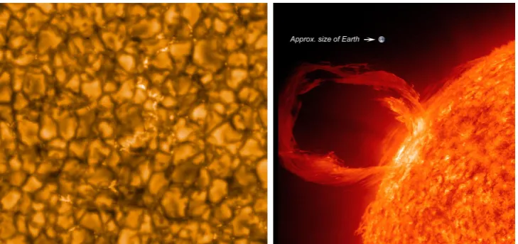
in the upper atmosphere. Taken from Kelvinsong (2012). . . 3 1.3. On the left side: Solar granulation. Courtesy of

JAXA/NASA/P-PARC (2010). On the right side: Solar flare. Courtesy of NASA/SDO (2016). . . 4 2.1. Illustration of the local domain used for the model in correlation to

the solar region that is subject to investigations. . . 16 2.2. Example background density and temperature profiles. a)

Temper-ature profiles for different θ, that were used. b) Density profiles for

θ = 2 but three different polytropic indices m. For these indices m

the atmosphere is stably stratified. . . 18 3.1. The velocity profiles considered by Reynolds (1883). (a) Velocity

pro-file without an inflection point. (b) Velocity propro-file with an inflection point. . . 36 3.2. Simple systems for a KH instability. (a) An interface with different

density and velocity at the top layer and bottom layer is shown. (b) A three layered system, where the middle layer has a continuously changing velocity and density ρ1. The top layer has a constant

ve-locity U1 with a lower density and the bottom layer has a constant

(8)

LIST OF FIGURES

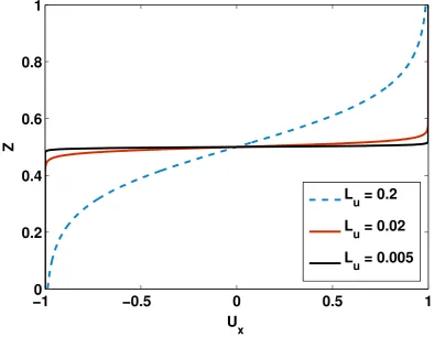
3.3. Example background shear flow profiles for three different Lu. Shear

flow profiles with very small and very large characteristic length Lu

for comparison. . . 43 3.4. Critical Richardson number in a viscous fluid withµ= 10−6for

differ-ent Mach numbers, M. The corresponding wave numberskmax of the

most unstable mode at the onset of instability are plotted, and the wave number is normalised by the inverse of the characteristic length 1/Lu. The horizontal line in both plots corresponds to Ri = 0.25.

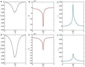
(a) Weakly stratified atmosphere with θ = 2. (b) Strongly stratified atmosphere,θ = 10. . . 52 3.5. Eigenfunctions for a fixed M = 0.1 and a fixed characteristic

length-scale Lu = 0.05 are found for two different θ, where θ = 10 for top

plots a, b, c and θ = 2 for the plots d, e, f. In both cases the eigenfunctions for δw, δT and δρ for the most unstable mode are shown. . . 54 3.6. Both plots show the growth rates ζ in a weakly thermally stratified

atmosphere with θ = 0.5 for a Richardson number of Ri = 0.22. (a) the fluid is compressible with M = 0.09. (b) M = 0.009, which corresponds to a incompressible fluid. The P´eclet number is varied among three orders of magnitude. . . 56 3.7. Plots of critical Richardson numbers for all k in a viscous fluid with

a Mach number,M = 0.009, a) θ = 0.5 and b)θ = 2.0 and viscosity

ν = 1×10−7_{. The P´}_{eclet number is varied from 10 to 0.01. . . .} ₅₉

3.8. Growth rate of the instability for a viscous fluid with θ = 2.0 and a Mach number of order 10−2_{. In (a) and (c) the P´}_{eclet number is}

P e = 1. In (b) and (d) P e = 0.1. Ri is varied in (a) and (b), but

Ri= 0.22 for the top plots (c) and (d). . . 60 3.9. Characteristics of instabilities for a viscous fluid with θ= 1.0, P´eclet

number of order 103 _and _Ri _{= 0}_._{3. (a) Growth rates. (b)}

(9)

4.1. Vertical velocity perturbations for different forcing methods just at the end of the exponential growth regime. (a) The viscous method. (b) The averaged relaxation method with τ0 = 10. (c) The averaged

relaxation method with τ0 = 0.1. (d) The local relaxation method

with τ0 = 10 and in (e) with τ0 = 0.1. . . 75

4.2. The time evolution of the volume averaged vertical velocity, as defined in Equation (4.10), for the two-dimensional calculations for case I in (a) and for case II in (b). Different τ0 parameters for the relaxation

method are used and compared to the viscous method and unforced calculations. The vertical velocity is displayed in logarithmic scale and t is given sound-crossing time. . . 76 4.3. The time evolution of the volume averaged vertical velocity for case

I with the local relaxation method. (a) Cases with τ0 ≤1. (b) Cases

with τ0 > 1. The vertical velocity is displayed in logarithmic scale

and t is given sound-crossing time. . . 78 5.1. The time evolution of the volume averaged vertical velocity, similar

to the definition in Equation (4.10) but for three-dimensional calcula-tions. Differentτ0 parameters for the relaxation method are used and

compared to the viscous method. The vertical velocity is displayed in logarithmic scale and t is given sound-crossing time. . . 85 5.2. The vorticity component perpendicular to the x-z-plane for different

forcing methods at two different stages during the time evolution. The plots at the top (a) and (b) show snapshots of two different times for the viscous method, where (a) is at ˜t = 7.2 and (b) at ˜t = 40. The middle row (c) and (d) show the relaxation method with τ0 = 10 at

˜

t= 6.8 and ˜t= 40, respectively. In (e) and (f) the relaxation method with τ0 = 0.1 was used, where ˜t= 12.3 in (e) and ˜t = 38 in (f). . . 86

5.3. The vertical velocity component,w, for different forcing methods after saturation. (a) Viscous method at ˜t ≈ 40. (b) Averaged relaxation method withτ0 = 10 at ˜t≈40. (c) Averaged relaxation method with

(10)

LIST OF FIGURES

5.4. Turbulent Reynolds number and length-scales for three different forc-ing methods. (a) Ret, as defined in Equation (5.12). (b) Turbulent

length-scales, lt. The red line indicates the horizontal extent of the

domain. . . 91 5.5. The horizontally averaged uxprofiles att≈60 are shown for different

forcing methods. . . 92 5.6. The total kinetic energy, internal energy and the gravitational

poten-tial energy evolution for the viscous forcing and relaxation method by using two different τ0. All energies are normalised by the

ini-tial total amount of the system’s energy Etot(t = 0) = 195.81. (a) Ekin(t)/Etot(t = 0) with time. (b)I(t)/Etot(t = 0). (c)Epot/Etot(t=

0). . . 95 5.7. The available gravitational potential energyEavail(t)/Etot(t = 0)

evo-lution for both the viscous forcing and relaxation methods by using two different τ0. . . 98

5.8. Time evolution of the viscous dissipation rate of momentum, ε, and the work done by the forcing,W. (a) Viscous forcing. (b) Relaxation method with τ0 = 10. (c) Relaxation method with τ0 = 1.0. . . 100

6.1. Density deviation from the initial background density profile, δρ. (a) The profiles at ˜t ≈ 60 for case I and different relaxation times. (b) Case II is displayed at ˜t≈250. . . 107 6.2. The minimal effective Richardson number obtained from the

horizon-tally averaged profiles as in Equation (6.1) with time. (a) Case I using two different relaxations times τ0. (b) Case II with three different

re-laxation timesτ0. The red line indicates the 1/4 stability threshold. . 109

(11)

6.4. Total vorticity in the x-z-plane for case A to C (see Table 6.2). The left column show cases A to C during saturation at approximately ˜

t ≈ 93. (a) Case A. (c) Case B. (e) Case C. The right column show the same cases during the quasi-steady state at different times (for reference see Fig. 6.3). The dotted lines indicate the extent of the turbulent region of the saturated state as obtained from Equation (4.13).116 6.5. The horizontally averaged and time averaged ¯ux profiles are shown

for cases A to H and O to U. In (a) the ¯ux(z) is displayed for cases A

to C in (b) the ¯ux(z) for cases D to H are shown. . . 117

6.6. The total vorticity component perpendicular to the x-z-plane shortly after saturation. Dotted lines indicate Lef f. (a) case D. (b) case F.

(c) case H where the red lines indicate the lower bound of the error for Lef f. . . 120

6.7. The temperature fluctuations around the initial temperature profile shortly after saturation. (a) Case D. (b) Case F. (c) Case H. Note, the scale in (c) is of one order of magnitude greater, such that small scale disturbances at the middle are not visible. . . 121 6.8. The total vorticity component perpendicular to the x-z-plane. (a)

case 3D-II at roughly ˜t≈200. (b) case 3D-I at roughly ˜t≈120. . . . 127 6.9. The ¯ux(z) for the diffusive instability cases. . . 131

6.10. The vorticity component perpendicular to the x-z-plane, the vertical velocityw, and temperature fluctuations around the initial tempera-ture profile for case Q long after saturation. (a) Vorticity. (b) Vertical velocity. (c) Temperature fluctuations. . . 132 7.1. A sketch of the scenario for potential tachocline dynamos, where the

stages are explained in the text. Taken from Priest (2014). . . 143 7.2. Schematic illustration of the structure in different main-sequence

(12)

LIST OF FIGURES

7.3. Magnetic energy with time together with and exponential curve fit. a) Case 2a and case 2b, which have low Prandtl numbers. b) The two large Prandtl number cases 2c and 2d. . . 151 7.4. Turbulent Reynolds numbers and typical length-scales with depth.

The vales are horizontally and time averaged during the saturated regime for all three cases and different forcing methods. (a) Ret(z).

(b) lt(z). . . 152

7.5. Magnetic energy evolution for case 3b and case 3c. . . 153 7.6. Time averaged relative helicity, H (z), as defined in Equation (7.9)

for all cases. a) Helicity obtained for case 1 and for all three different forcing methods is shown. b) Helicity for case 2 to case 4 is displayed. 154 7.7. Magnetic energy density evolution with time for large magnetic

Prandtl numbers of case 4. a) Case 4d with σm = 10. b) Case

4e. c) Case 4f. . . 155 7.8. Time evolution of Bmean for the cases 4d and 4e with time. . . 157

7.9. Time evolution of the horizontal magnetic field components hBxiand hByifor the cases 4d and 4e with time. . . 157

7.10. Γ(z) as a function of depth and time for case 4e. . . 158 D.1. Illustration of a sorting procedure for an array, which is distributed

(13)

List of Tables

4.1. Comparing the linear eigenvalue-solver results with those from non-linear calculations during the non-linear phase. For case I the shear am-plitude isU0 = 0.08 and 1/Lu = 118 such thatRi = 8×10−4. Taking Ck = 8×10−5 results in aP e≈8. For case IIU0 = 0.041, 1/Lu = 20

and Ck = 1×10−4 such thatRi = 0.1 and P e≈20. . . 71

5.1. Time intervals of the different dynamical stages. . . 93 6.1. Parameters for the investigated cases, where the resolution of the

domain is given by Nx, Ny and Nz. The dynamical viscosity is Ckσ,

where Ck is the thermal diffusivity and σ the Prandtl number. The

temperature gradient is denoted as θ and the polytropic index is m. For the initial shear flow the shear amplitude is U0 and the shear

width is controlled by Lu. . . 106

6.2. Comparing typical length-scales, turbulent Reynolds numbers and ef-fective shear width Lef f for different transport coefficients. For cases

A to H the initialRi number is fixed to be 0.006, whereθ = 1.9, the polytropic index ism= 1.6, the shear amplitudeU0 = 0.095, and the

shear width is Lu = 0.016. The effective shear width is calculated

after saturation and Re¯t, P e¯t, and ¯lw are averaged in the turbulent

region, which depends on the effective Lef f, and over a sufficiently

(14)

LIST OF TABLES

6.3. For all cases Lu = 0.016 and σCk = 1.0×10−4. For cases I to K the

temperature gradient is varied from θ = 0.85 to θ= 6.5. For cases L to N the P´eclet number is varied, butRi= 0.006. The effective shear width Lef f is calculated as described in Section 4.3. All turbulent

quantities are averaged in time and over the turbulent region indicated byLef f. . . 113

6.4. For the diffusive instability cases O to U the temperature gradient,

θ = 2.0, and the polytropic index, m = 3.0, are fixed, but the initial

Ri number changes from 0.4 for cases O to Q to 1.0 for case U. The effective shear width is calculated after saturation and ¯Ret, ¯P et, and

¯

lw are averaged in the region of the turbulence, depending on the

effective Lef f. . . 130

7.1. The values of various parameters for all cases considered together with the decay rates for each. For all cases the polytropic index is set to

m = 1.6 and the dynamic viscosity µ = 5×10−4_{. In part 1}

(15)

Acknowledgements

The last years, during which I worked on my PhD research project, brought many positive changes to my life and I am very grateful for that. This would not have been possible without many people all over the world, their support, motivation and inspiration.

First and foremost I want to express my sincere gratitude to my supervisor Dr Lara Silvers. I appreciate all her contributions of time, ideas, and funding to make my PhD experience productive and stimulating. Her enthusiasm for research is contagious and motivated me, even during tough times in my PhD. I am also thankful for the excellent example she has provided as a successful woman in math-ematics.

I would like to gratefully and sincerely thank Dr Benjamin Favier, who has been a truly dedicated mentor and collaborator, for his tremendous academic support and fruitful discussions. This research project would not have been possible without his permanent guidance and support.

I would also like to take this opportunity to thank my viva examiners Dr Oliver Kerr and Professor Steve Tobias for helpful comments and suggestions.

Very special thanks to all colleagues in the Department of Mathematics for their advice, collaborations and creating a pleasant working atmosphere. Additionally, I am very thankful for the friendship of all other PhD students in our office. Especially, I am indebted to Niamh and Laura for numerous discussions during our lunch breaks and their support.

(16)

LIST OF TABLES

Declaration

(17)

Abstract

Shear flows have a significant impact on the dynamics in various astrophysical ob-jects, including accretion discs and stellar interiors. Due to observational limita-tions the complex dynamics in stellar interiors that result in turbulent molimita-tions, mixing processes, and magnetic field generation, are not entirely understood. It is therefore necessary to investigate the inevitable small-scale dynamics via numeri-cal numeri-calculations. In particular a thin region with strong shear at the base of the convection zone in the Sun, the tachocline, is believed to play an important role in the Sun’s interior dynamics and magnetic field generation. Velocity measurements suggest a stable tachocline. However, helioseismology can only provide large-scale time-averaged measurements, so small-scale turbulent motions can still be present. Therefore, studying the stability of shear flows and their non-linear evolution in a fully compressible polytropic atmosphere provides a fundamental understanding of potential motion in stellar interiors and is the main focus of this thesis.

(18)

1. Introduction

The aspiration of mankind to understand nature has given rise to many scientific areas. One of them, astrophysics, is the study of celestial objects, such as planets, stars, and galaxies. A specific characteristic of astrophysics research is the method by which we obtain information on the object of interest: Since astrophysical objects are distant, the only way to measure their properties is to observe and investigate all types of radiation they emit. Therefore, detailed observations are difficult, even for our Sun (see Hansen and Kawaler, 1999a, and references therein). To enhance our understanding of these objects it is imperative to use analytical and numer-ical techniques in addition to observations. Using mathematnumer-ical models requires appropriate assumptions to simplify the system in order to shed light on particular aspects. Therefore, numerical results have to be compared with available observa-tions in order to be verified and to improve the current models. Before moving on to discuss numerical modelling in detail, it is crucial to gain a general picture of astrophysical objects.

Stars

(19)

The luminosity remains constant with distance per definition, and so it is an intrinsic quantity of a star (Karttunen et al., 2007).

Taking a closer look reveals that stars have different colours, where one possible system of classification is made by distinguishing three colours. Here filters are used to obtain the magnitude of a star in the colours ranging from ultraviolet (U) to blue (B) and to visual (V). Depending on the difference of magnitude between U to B and B to V, stars are categorised into different spectral types (Karttunen et al., 2007). The spectral types range from very hot stars of type O over B, A, F, G and K to the coolest stars of type M. For example, yellow and red stars belong to the spectral types G-K-M. Our Sun is a G type star with the full classification, G2 V (Karttunen et al., 2007).

[image:19.595.141.510.423.698.2]

In the early 19th century a study of the relationship between the absolute magnitude of a star and its spectral type led to the well known Hertzsprung-Russell diagram (see Fig. 1.1).

(20)

Despite a potential uniform distribution in such a diagram, the investigations re-vealed that most stars are located on a diagonal curve, the so called main sequence (Karttunen et al., 2007). However, there are several other branches, as for example the horizontal branch, the red giants, the super-giants and the white dwarfs. The different branches correspond to different stages of stellar evolution, where not every star follows through the same stages (Karttunen et al., 2007). Dense regions rep-resent evolution phases in which stars remain a long time. Since stars in the main sequence have similar interior structure and dynamics, our Sun, which is roughly at the middle of the main sequence, is a representative example of such stars.

Structure of the Sun

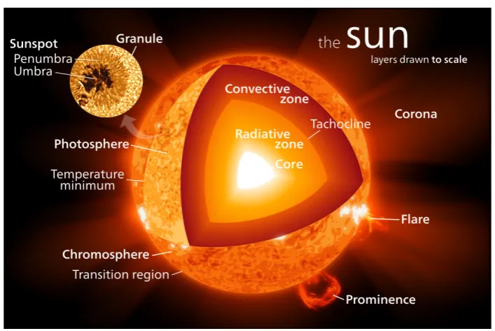
[image:20.595.149.503.394.631.2]

Our Sun has been a prominent object of investigations since 2000 B.C. (Priest, 2014). Nowadays, it is known that the Sun is a giant gas sphere with a complex underlying structure, which is divided into different layers, as illustrated in Fig. 1.2. The outer regions of the Sun are the corona, the chromosphere, and the photosphere.

Figure 1.2.: Sun’s structure. Illustration of stellar layers and phenomena occurring in the upper atmosphere. Taken from Kelvinsong (2012).

(21)

[image:21.595.145.510.454.626.2]

Such dark spots are regions of lower temperature than their surroundings and are called sunspots. The systematic investigations of sunspots started in 1610. At that time, Galileo and others began to use telescopes to record the number of sunspots (Hathaway, 2010), which eventually revealed a periodic behaviour of the sunspot activity. Much later, the emergence of sunspots was linked to underlying magnetic field evolution (Solanki, 2003), which demonstrates the complex interaction of solar processes. More comprehensive investigations started in the 19th century, where even the fine structure, called granulation (see Fig. 1.3), of the photosphere could be resolved by Langley (Priest, 2012). Such observations led to the discovery of abruptly occurring bright flashes, the so called solar flares. Solar flares, shown in Fig. 1.3, are often followed by bright, mostly loop shaped, gas patterns propagating outwards into the solar corona (Fletcher et al., 2011). These eruptions are solar prominences and are usually accompanied by coronal mass ejections (Schmieder et al., 2008). Nowadays, in order to investigate the composition of elements, densities and temperature in outer solar regions, various measurements using spectroscopic techniques are conducted (Appenzeller, 2012).

(22)

re-gions of the Sun, which are difficult to observe and are not entirely understood. The inner part of the Sun can be divided into the convection zone, the radiative zone, and the core. These regions obtained their names due to their energy trans-port properties: The convection zone is dominated by convective transtrans-port. The leading transport in the radiative zone is radiation and the core provides the energy source (D. H. Hathaway, 2015). Unlike the Sun’s atmosphere, the convection zone, the radiative zone and the Sun’s core are optically thick (Lopes, 2002). Therefore, electro-magnetic waves cannot escape this region, and optical observations are im-possible. In order to obtain information of the structure and dynamics in these regions, measurements of acoustic wave propagation need to be used (Gough et al., 1996). This technique is called helioseismology. So far helioseismology can only pro-vide time averaged measurements with rather low resolution (Christensen-Dalsgaard and Thompson, 2007).

However, these observations together with preceding theoretical conclusions allow one to draw the following picture: Beneath the solar surface the convection zone is located, where convectional flows as well as turbulent motions are predominant. These dynamics reach down to the recently discovered tachocline (Kosovichev et al., 1997; Tobias, 2004), which separates the convection zone from the very distinct radiative zone. The radiative zone, which is stably stratified, rotates as a solid body, but above this region, in the convection zone, differential rotation is present. A region with strong differential rotation, the so-called tachocline, is needed to match the rotational dynamics of these two regions (Spiegel and Zahn, 1992; Goode et al., 1991). Global properties of the tachocline like the thickness and approximate location between 0.67R, whereRis the solar radius, and 0.72Rwere determined

by helioseismic observations (see for example Kosovichev, 1996; Charbonneau et al., 1999; Arlt, 2009). However, approximations on the radial extent of the tachocline range from 0.019 R (Charbonneau et al., 1999) to 0.039 R (Elliott and Gough,

1999), which demonstrates the insufficient accuracy of measurements.

Magnetic Fields and Gas Dynamics

(23)

in-of high-priority, since the inner gas dynamics also play a crucial role in magnetic field generation (Hughes et al., 2007). In general, magnetic fields are generated as soon as there are electrically charged particles present and not at rest, which was established by the Amp`ere’s Law in 1825 (Jackson, 1975). As electrons have a mag-netic dipole moment due to their spin, magmag-netic fields are present everywhere on sub-atomic scales (Dirac, 1958). However, such magnetic fields are randomly dis-tributed. Therefore, to obtain magnetic fields that are structured on scales larger than sub-atomic scales, additional mechanisms are needed (Davidson, 2001). De-spite the complex dynamics required to generate and sustain structured magnetic fields, they have been observed in most astrophysical objects, such as galaxies, stars and some planets on scales comparable to the size of the object (Kardashev, 1992). Solar magnetic fields were discovered in 1908 by Hale (Solanki, 2003). One of the successful ideas to explain these observations was by Sir Joseph Larmor (Ruzmaikin et al., 1988). His main statement, that magnetic fields are a general feature in large rotating astrophysical objects due to a dynamo process, initiated an extensive study of the interior dynamics in galaxies, stars and planets.

In this context, the strong shear flow in the tachocline region is believed to play a curial role in the process of generating magnetic fields (see Parker, 1993; Silvers, 2008, and references therein). However, a consistent model is still absent, due to a lack of understanding of the small-scale and large-scale dynamics. Because of the absence of detailed observations in such regions, analytic and numerical techniques are required to shed light on the motions present. Therefore, the focus of this thesis is to exploit numerical calculations to study shear flows in stellar objects.

Shear flows

(24)

settings for us to understand the evolution of the shear flows inside the Sun. There-fore, we must start from a pure hydrodynamical system in our modelling to build up a comprehensive understanding, before including magnetic fields.

Previous studies of shear flows have shown that such flows can undergo what is known as the Kelvin-Helmholtz (KH) instability, which develops due to the con-version of the available kinetic energy of the shear flow into kinetic energy of the disturbances (see Drazin and Reid, 2004, Chap. 6). In addition to the KH instability, other instabilities, such as baroclinic instability (see Charney, 1947) or the Holmboe instability (Holmboe, 1962), can appear when flows are either rotating or stratified. For the study in this thesis the latter one is of greater interest for following reason: While the KH instability is suppressed by stratification, the more slowly growing Holmboe modes become dominant with increasing stratification (Peltier and Smyth, 1989).

(25)

the appearance and consequences of a Holmboe-like instability is investigated. A linear stability analysis is not sufficient to understand the dynamics of shear flows such that three dimensional direct numerical calculations are required to investigate non-linear evolution. In the existing literature most numerical studies of the turbu-lence transition in shear flows take the approach of an unforced flow (Caulfield and Peltier, 2000; Smyth and Moum, 2000; Smyth and Winters, 2003), which results in a finite lifetime of an unstable mean state. However, the tachocline is not a transient feature such that physical mechanisms are present by which the flow is sustained. The resulting force acting on the flow is not known in detail. Thus investigations of astrophysical shear flows utilise different methods to reach a sustained flow.

In the context of stellar dynamics, global-scale calculations of stellar interior dy-namics investigate the mechanism to maintain differential rotation by body forces resulting from viscous stresses, Reynold stresses and meridional circulation (Brun and Toomre, 2002; Miesch et al., 2008). Because in this work the investigations aim to model a local region of differential rotation in stellar interior, it is of twofold interest to choose a suitable method to maintain a target shear profile. First, the effect of different forcing methods on the evolution of turbulence can be investigated; and second, a comparison with results obtained by global-scale calculations can be drawn. Therefore, a comparative analysis of different forcing methods is the second part of this thesis. Finally, the last two parts of this thesis focus on the question of how modelling shear flows can help us to understand the complex dynamics and interaction of matter and magnetic fields in stellar interiors.

Outline

(26)

(27)

In search of a better understanding of dynamical processes in a particular system, it is necessary to formulate an appropriate model. In this chapter we start by reviewing some basic properties of solar-like stars in Section 2.1 in order to verify the choice of the basic state, the boundary conditions and geometry of the numerical domain. In Section 2.2 the set of governing equations for a pure hydrodynamical problem and its non-dimensional form is derived. For the magnetohydrodynamical problem, the principal assumptions of the induction equation and the complete set of differential equations are shown in Section 2.3. Finally, the numerical methods used to solve the set of differential equations are described in Section 2.4.

2.1. Stellar Properties

To numerically model stellar interior dynamics it is crucial to first examine stellar properties. In order to approximate the inner structure in real stars, static stellar models were considered, which obey the spherical symmetry of the system (Cox and Giuli, 1968). For this, two fundamental assumptions were made to model a stable homogeneous star. The first assumption is that mass changes with radius according to

dM(r)

dr = 4πr

2_ρ₍_r₎_, _(2.1)

whereM(r) is the mass within the radiusr,ρ(r) the density. The second assumption is due to the requirement that the star is stable and so it needs to be in a hydrostatic equilibrium

dp(r)

dr =−

GM(r)

r2 ρ(r) = −g(r)ρ(r), (2.2)

(28)

2.1. STELLAR PROPERTIES

and the density needs to be considered. For most stars it is convenient to assume that the pressure depends only on the density such that a polytropic relation

P =Kρ1+1/m, (2.3) where m ∈ _R+ _{is the polytropic index and} _K _{is an arbitrary constant, can be}

assumed (Cox and Giuli, 1968). These equations form the earliest stellar models, where it is assumed that a star is a polytopic gas sphere with self gravity (Collins, 2003). After introducing dimensionless variables

ρ=ρcθm, P =Pcθm+1, r =αξ, α=

r

m+ 1 4πG Kρ

1/(m−1)

c , (2.4)

where θ is the polytropic temperature, and combining Equations (2.1) - (2.3) the Lane-Emden equation can be derived,

1

ξ2

d dξ

ξ2dθ dξ

=−θm. (2.5) The order of the solutions for the Lane-Emden equation is determined by the poly-tropic indexm, such that it can be distinguished between several cases. Form = 0, the solution corresponds to an incompressible sphere, where the density remains constant with the radius. In the range 1≤m≤1.5 the solutions obtained represent a superadiabatic atmosphere that is unstable to convective motions, which is the case for the convection zone or fully convective stars (Cohen, 2009). For m > 1.5 the stratification is subadiabatic such that the atmosphere is stable against convec-tion. A special case is m = 3, which corresponds to the Eddington approximation and for m >5 the solutions cannot be used to model a star, because the radius of such a star becomes infinite.

(29)

and which layer of a star is modelled, is crucial in order to decide which type of basic state is required.

The substantial part of main-sequence stars is formed by the stellar core and the ra-diative zone, which exhibit the energy source of a star and where energy transport is due to radiative processes (Pradhan and Nahar, 2011). Above the radiative zone the stratification becomes super-adiabatic such that energy transport is predominately by convective motions. These two layers, the radiative zone and the convection zone, are separated by a thin region, the tachocline. This intermediate region is of particular interest, because it has a significant impact on magnetic field generation. Therefore, it is important to explore the known properties of this region.

Although, for other stars the location and properties of the tachocline are unknown, some information is available for the Sun, as helioseismology keeps constantly en-hancing the measurement’s accuracy. However, it is difficult to make assumptions about the precise shape of the shear flow, because the available measurements for the solar tachocline are not sufficient to resolve the velocity profile on small scales, such that only time averaged large-scale measurements can be provided (Christensen-Dalsgaard and Thompson, 2007). In the Sun, the tachocline overlaps with the base of the convection zone especially in regions of higher latitudes (Basu and Antia, 2001; Forg´acs-Dajka and Petrovay, 2002). The radiative envelope, located just be-neath the tachocline, has an angular velocity Ω0 = 2π×463 nHz (Gough, 2007),

i.e. assuming the top of the radiative envelope at 0.67R this results in a velocity

of 1.36 kms−1. The change of velocity across the tachocline was approximated to be ∆u≈50ms−1 _{(Soward et al., 2005), such that taking the speed of sound at 0.7} _R

into account, the Mach number for the mean flow in the tachocline is about 0.005. In order to understand the stability of the tachocline the Richardson number can be approximated from temperature and density profiles. The stratification changes from sub-adiabatic in the radiative envelope to super-adiabatic in the convection zone. Using Table 1.1 in Gough (2007) and considering a polytropic atmosphere, it is possible to calculate the polytropic index at 0.7R to be roughly 2.0, which

(30)

2.1. STELLAR PROPERTIES

upper part of the tachocline, which suggests a stable shear flow. Furthermore, by taking the thermal diffusivity κ the P´eclet number can be estimated to be of order 106 _{to 10}7_.

The transport coefficients are known to a greater accuracy throughout the solar interior. However, numerical calculations are incapable of reaching the correct order of magnitude of transport coefficients due to the numerical cost of performing at such low viscosity and thermal diffusivity. Therefore, it is necessary to verify the applicability of numerical calculations performed at different transport coefficients, respecting certain ratios. A more detailed discussion can be found in Chapter 6, where possible effects on the resulting dynamics are studied.

Setting up the model

(31)

2.2. Hydrodynamics

A hydrodynamical description of the system involves the continuum hypothesis, which assumes a continuous medium (Wesseling, 2009), and is valid for stellar in-teriors. Furthermore, for the Navier-Stokes equations, which form a macroscopic hydrodynamic description, the hydrodynamical approximation has to be applica-ble. This is provided, if for any given time the system remains in a thermodynamic equilibrium, such that the relaxation time towards an equilibrium is less than the smallest time increment. If this condition is satisfied, hydrodynamical characteris-tics such as temperature and density can be defined. In the region of interest the gas constituents behave as if they are in a thermodynamic equilibrium (Hansen and Kawaler, 1999b), such that the following macroscopic description is valid.

The set of differential equations can be obtained by considering conservation laws. The first conservation law concerns the mass conservation. It states that the change of density within a certain volume dV is equal to the outflow through the surface,

dS, for a closed system, i.e.

∂ ∂t

Z

V ρdV

=−

I

S

ρu·ˆndS, (2.6) whereρis the density,u the velocity field and ˆnis the normal vector to the surface. The minus sign is convention due to the normal vector pointing outwards. Then using the divergence theorem the continuity equation takes the form

∂ρ

∂t =−∇·(ρu). (2.7)

The Navier-Stokes equation arises from the momentum conservation for a fluid par-cel. The momentum change of a fluid parcel is equal to the sum of all forces acting on it. Then, the general form is given by

ρDu

Dt =∇ ·o+f, (2.8)

(32)

2.2. HYDRODYNAMICS

Making use of the continuity equation and rewriting the total derivative as the Lagrangian frame derivative leads to

∂ρu

∂t +∇·(ρuu) =∇ ·o+f. (2.9)

The stress tensor can be decomposed into the surface pressure and the viscous stresses, and the only body force considered is gravity, such that the Navier-Stokes equation becomes

∂ρu

∂t +∇·(ρuu) =−∇P +gρ+µ∇·τ, (2.10)

where P is the pressure, g the gravity and τ the strain rate tensor. The dynamical viscosity is denoted by µ.

Finally, from energy conservation the heat equation (or temperature evolution equa-tion) is derived, which is obtained by equating the total change of temperature, T, with all sinks and sources,

ρ∂T

∂t +ρu·∇T = γκ∇

2

T

| {z }

thermal diffusion

+µ(γ−1) 2 |τ|

2

| {z }

viscous heating

−ρ(γ−1)T∇·u

| {z }

work by compression

, (2.11)

where κ is the thermal conductivity and γ = cp/cv denotes the adiabatic index,

which is the ratio of the heat capacities cp at constant pressure, and cv at constant

volume. The thermal diffusion term was obtained by assuming a constant thermal conductivity throughout the domain. In this thesis the fluid is assumed to be an ideal gas, such that the equation of state is

P =RspecρT, (2.12)

where Rspec is the specific gas constant.

2.2.1. Non-dimensional Governing Equations

(33)

[image:33.595.153.500.116.339.2]

and z = d are impermeable. The horizontal directions, x and y, are periodic (see Figure 2.1 for an illustration of the domain). The fluid is assumed to be an ideal gas

Figure 2.1.: Illustration of the local domain used for the model in correlation to the solar region that is subject to investigations.

with constant dynamic viscosity µ, constant thermal conductivity κ, constant heat capacities cp at constant pressure, and cv at constant volume. In order to obtain

non-dimensional equations for the system under consideration, the fundamental unit of length is the domain depth d. Furthermore, fundamental units of temperature and density are set to beTtandρt, which correspond to the temperature and density

at the top boundary, and results in the fundamental pressurePt= (cp−cv)ρtTt. The

time is normalised by the sound crossing time, which is ˜t=d/[(cp−cv)Tt]1/2 for the

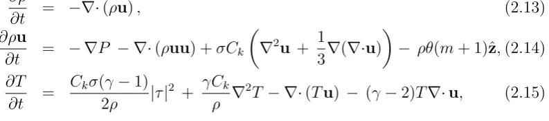
chosen fundamental units. Then the equations, in non-dimensional form, are

∂ρ

∂t = −∇·(ρu), (2.13) ∂ρu

∂t = − ∇P − ∇·(ρuu) +σCk

∇2_u ₊ 1

3∇(∇·u)

− ρθ(m+ 1)ˆz,(2.14)

∂T

∂t =

Ckσ(γ−1)

2ρ |τ|

2 ₊ γCk

ρ ∇

2_T _{− ∇·}₍_T_u₎ ₋ ₍_γ₋₂₎_T_∇·_u_, _(2.15)

whereθdenotes the temperature gradient and mis the polytropic index. Due to the fundamental units the following non-dimensional numbers are used. The dimension-less Prandtl number,σ =µcp/κ, is the ratio of viscosity to thermal conductivity and

[image:33.595.144.541.593.681.2]

(34)

2.2. HYDRODYNAMICS

of both results in the non dimensional dynamical viscosity. Because a Newtonian fluid is considered, the strain rate tensor has the form

τij = ∂uj ∂xi

+ ∂ui

∂xj −δij

2 3

∂uk ∂xk

. (2.16)

2.2.2. Boundary Conditions and Background State

As discussed in Section 2.1 a polytropic relation between pressure and density has to be assumed, where the pressure is a function of density only i.e.

P(ρ) ∝ ρ(1+m1), (2.17)

where m is the polytropic index. Due to the Schwarzschild criterion the fluid is stable against convection if the inequality m >1/(γ−1) holds, where the adiabatic index, γ, is equal to 5/3. Then, the system is convectively stable for a polytropic index of m >1.5. Only stable stratified atmospheres will be considered throughout this thesis.

Boundary conditions, at the top and bottom of the of the domain, are impermeable and stress-free velocity i.e.

uz = ∂ux

∂z = ∂uy

∂z = 0 at z = 0 and z = 1 (2.18)

and fixed temperature, which means:

T = 1 at z = 0 and T = 1 +θ at z = 1. (2.19) To include thermal effects it is necessary to choose the background temperature in such a way, that it is a stationary solution of the heat equation or remains quasi-stationary on time-scales larger than the thermal diffusion time-scale. This results in a temperature and density profile of the form:

(35)

Some background profiles for temperature and density are shown in Fig. 2.2.

0 0.1 0.2 0.3 0.4 0.5 0.6 0.7 0.8 0.9 1

0 5 10 15 a)

Z

T

0 0.1 0.2 0.3 0.4 0.5 0.6 0.7 0.8 0.9 1

0 10 20 30 b)

Z

ρ

0 0.1 0.2 0.3 0.4 0.5 0.6 0.7 0.8 0.9 1

−1 −0.5 0 0.5 1 c)

Z

U x

θ = 0.5

θ = 2

θ = 10

θ = 2 ; m = 1.6

θ = 2 ; m = 2.0

θ = 2 ; m = 3.0

L u = 0.2 L

[image:35.595.130.503.111.403.2]

u = 0.007

Figure 2.2.: Example background density and temperature profiles. a) Temperature profiles for different θ, that were used. b) Density profiles for θ = 2 but three different polytropic indicesm. For these indicesmthe atmosphere is stably stratified.

2.2.3. Important Approximations

(36)

2.2. HYDRODYNAMICS

thermal effects rather than from pressure and in the momentum equations density fluctuations are neglected except their coupling to the gravitational term.

(37)

2.3. Magnetohydrodynamics

Stellar interiors consist of plasma. Therefore, the equations of magnetohydrody-namics (MHD) are required in order to fully model the dymagnetohydrody-namics. The set of MHD equations is similar to the set of differential equations derived for the pure hydro-dynamical case in Section 2.2. However, additional terms that result from magnetic field coupling to matter need to be considered in the Navier-Stokes equation and temperature evolution equation. Furthermore, to describe the magnetic field evo-lution due to velocity fields and magnetic diffusion, the induction equation is needed. To begin to obtain the full MHD equations, the induction equation is derived from the Maxwell equations, which are the fundamental equations of classical electrody-namics:

∇ ·E = 4π%e, (2.22) ∇ ·B = 0, (2.23)

∇ ×E = −1

c∂tB, (2.24)

∇ ×B = 1

c(4πJ+∂tE), (2.25)

where E is the electric field and B is the magnetic field. The electrical charge density is denoted by %e, c is the speed of light and J is the electrical current

density. In addition to these equations, Ohm’s Law has to be considered. It states that in a frame of reference that is at rest J =σ0E holds, where σ0 is the electrical

conductivity. As here the frame of reference is moving with the fluid with a speed

u, it is necessary to perform a coordinate transformation under which the resulting electrical current remains unchanged. This description leads to the additional term

u×B, because the electric field transforms asE=Er−u×B, when the frame of

reference is changed. Then Ohm’s Law becomes

J =σ0

E+1

cu×B

. (2.26)

(38)

2.3. MAGNETOHYDRODYNAMICS

the electric conductivity in a plasma is very high, such that no electrical potential is present on scales larger than the Debye length. This also follows from applying the magnetohydrodynamical approximation. Following the discussion in Kippen-hahn and M¨ollenhoff (1975) to obtain the magnetohydrodynamical approximation a parameterα is introduced and only terms up to linear order inα are kept. Higher order terms are neglected. For that, the first assumption is that only non-relativistic velocities are considered. So if settingL as a typical length-scale andt0 as the

typi-cal time-stypi-cale, the typitypi-cal velocity U0 =L/t0 has to be much less than the speed of

lightc. This leads to the above mentioned parameter α,

U0

c =

L/t0

c =α 1.

Then, assuming that electric and magnetic fields do not change significantly on a typical time-scale and typical length-scale, the spatial and time derivatives can be approximated as follows

∂E ∂t ≈ E to ∂E ∂x ≈ E L, ∂B ∂t ≈ B to ∂B ∂x ≈ B L.

With the above assumption, the third Maxwell Equation (2.24) requires that

E B = L/t0 c

=α1.

This is used to rewrite the fourth Maxwell Equation (2.25) as follows

B/L= 1

c4πJ+

1

cE/t0. (2.27)

This equation is rearranged as follows,

B= L

c4πJ+ L

c αB

t0

⇒ B= L

c4πJ+α

2

(39)

Equation (2.26) are of the same order and therefore both terms on the right-hand side remain. At this point it is straight forward to rewrite the third and fourth Maxwell equations together with the Ohm’s Law to obtain

∂tB=∇ ×(u×B)− ∇ ×

c2

4πσ0

∇ ×B

, (2.29) where the pre-factor c2_/₍₄_πσ

0) = η, which is the magnetic diffusivity. In this

par-ticular case, the magnetic diffusivity is assumed to remain constant throughout the domain, such that using the vector identity ∇ ×(∇ × B) = ∇(∇ ·B)− ∇2_B _the

induction equation becomes

∂tB =∇ ×(u×B) +η∇2B. (2.30)

The first term on the right-hand side corresponds to the response of the magnetic field to plasma motion and the second term describes the diffusion of the magnetic field.

Having the MHD approximation and the Maxwell equations in mind, it is possible to write down the Navier-Stokes equation that become of the form

∂ρu

∂t +∇·(ρuu) =−∇P +µ∇·τ +gρ+

1

µ0

(∇ ×B)×B

whereµ0 is the vacuum permeability and the last term comes from the Lorentz force

FLorentz =%e(E+u×B). Here the first term in the Lorentz force is negligible due

to the MHD approximation and the second term was rewritten by using the fourth Maxwell Equation (2.25).

For the temperature evolution equation, an energy loss has to be considered due to ohmic dissipation, which is represented as an additional term

ρ∂T

∂t +ρu·∇T =γκ∇

2_T ₊µ(γ−1)

2 |τ|

2₋_ρ₍_γ ₋₁₎_T_∇·_u_{+ (}_γ₋₁₎_η_|_J_|2

| {z }

ohmic dissipation

, (2.31)

(40)

2.3. MAGNETOHYDRODYNAMICS

2.3.1. Non-dimensional MHD Equations

Using the same fundamental units as used for a pure hydrodynamical system in the previous section the non-dimensional MHD equations are obtained. The resulting equations are (Matthews et al., 1995):

∂ρ

∂t = −∇ ·(ρu) (2.32) ∂ρu

∂t = −∇P

∗_{− ∇ ·}

(ρuu−fBB)−ρg+σCk

∇2_u₊ 1

3∇(∇ ·u)

(2.33)

∂T

∂t =

γCk

ρ ∇

2_T _{− ∇ ·}₍_T_u₎₋₍_γ₋₂₎_T_{∇ ·}_u _(2.34)

+Ck(γ−1)

ρ

σ

2|τ|

2

+f ξ|J|2, ∂B

∂t = ∇ ·(Bu−uB) +ξCk∇

2

B (2.35)

∇ ·B = 0, (2.36)

where the total pressure P∗ =ρT +f|B|2_/_{2 includes the magnetic pressure. Here,}

f = |B|2_/µ

0Pt gives the ratio of the magnetic pressure to the fundamental unit

pressure. Note, that only for calculations withf 6= 0 the magnetic field is normalised by the magnitude of the background magnetic field. Like in the previous section,

Ck = κ˜t/(ρ0cpd2) is the thermal dissipation parameter, σ = ν/Ck is the Prandtl

number and one additional non-dimensional parameter is introduced, the inverse Roberts number ξ = ηcpρt/κ. The inverse Roberts number represents the ratio of

the Prandtl number to the magnetic Prandtl number σM =ρ0µ/η. Like in the pure

hydrodynamic case, the strain rate tensor has the form as in Equation (2.16). In addition the magnetic field has to remain divergence free due to the non-existence of magnetic monopoles and therefore Equation (2.36) has to hold.

2.3.2. Boundary Conditions and Background State

(41)

For the magnetic field there exist two possible boundary conditions: One possibil-ity, the so called pseudo-vacuum (Favier and Proctor, 2013; Jackson et al., 2014), assumes the magnetic field to be normal to the boundary. Here the boundary con-ditions read

Bx =By =∂zBz = 0 at z = 0 and z = 1. (2.37)

For the second possibility the magnetic field is tangential to the boundary, such that

Bz =∂zBx=∂zBy = 0 at z = 0 and z = 1. (2.38)

This is also called a perfect electrical conductor (Favier and Proctor, 2013).

2.4. Numerical Methods

One major issue solving Navier-Stokes or MHD equations numerically is due to the demand of resolution of a rapidly increasing instantaneous range of scales with greater Reynolds numbers. The existing methods to solve the set of equations numerically can be classified into three categories; direct numerical simulations (DNS), large eddy simulations (LES) or Reynolds-averaged Navier-Stokes simula-tions (RANS) (Miki, 2008). DNS provide the most accurate approach due to their theoretical ability to resolve all spatial and temporal scales. In practice, DNS solves a reasonable subset of scales that ensure accuracy but to keep the computational cost low. The latter two methods come with approximations: The RANS solve for a statistical evolution of the quantities, where each quantity is decomposed into a mean value and a fluctuating part (Durbin and Reif, 2010). The LES employ filter functions to model a certain range of small-scales, but directly solves large-scales (Garnier et al., 2009). Therefore, DNS are suitable for addressing fundamental research questions that require high accuracy, as for example needed in turbulent flows.

2.4.1. Non-linear DNS Calculations

(42)

finite-2.4. NUMERICAL METHODS

difference/pseudo-spectral code is exploited, where a description can be found in Matthews et al. (1995). This code was further developed, optimised and used over the last two decades (see for example Matthews et al., 1995; Silvers et al., 2009a; Favier and Bushby, 2012, 2013, and references therein).

Since the computational domain that I will consider is a Cartesian box with imper-meable walls at the top and bottom and periodic boundary conditions in x- and y -directions, the following numerical methods to calculate spatial and time derivatives are used.

Vertical Derivatives

The derivatives in the vertical direction are obtained by using an explicit fourth-order finite-difference scheme. The finite difference method (FDM) is the oldest method and dates back to 1768, when it was applied by Euler (Hirsch, 2007a). For such a method the conservative form of the differential form of the equations is used. The basic idea behind this method is to use the definition of the derivative

∂f(x)

∂x = lim∆x→0

f(x+ ∆x)−f(x)

∆x (2.39)

together with the Taylor expansion

f(x+ ∆x) = f(x) + ∆x∂f(x)

∂x +

∆x2

2

∂2_f₍_x₎

∂x2 +

∆x3

3!

∂3_f₍_x₎

∂x3 +... (2.40)

+ ∆x

n−1

(n−1)!

∂n−1f(x)

∂xn−1 +O(∆x

n₎_,

which is expanded around f(x).

Assuming an uniformly discretised grid and rewriting Equation (2.40) the first derivative at the point i is

f_i(1) =

∂f ∂x

i

= fi+1−fi ∆x −

∆x

2 f

(2)

i − O(∆x

2₎

| {z }

truncation error

, (2.41)

where (m) _{denotes the} _mth _{derivative with respect to} _x_{and the subscript}

i+1 that it

(43)

itself and one neighbouring point to its right. Furthermore, the highest order in the truncation error is of order one. Since the accuracy order depends on the power of the truncation error, Equation (2.41) is the first order forward difference formula. It is also possible to derive the backward difference scheme and a centred formula. As an example calculation, the centred formula can be obtained by taking fi+1 and

fi−1 and subtracting them from each other:

fi+1−fi−1 = 2∆xf(1)+

2∆x3

3! f

(3)₊2∆x5

5! f

(5)₊_...₊ 2∆x2n+1

(2n+ 1)!f

(2n+1)₊_..., _(2.42)

Rearranging this equation, the general centred finite difference approximation be-comes

fi+1−fi−1

2∆x =f

(1)₊∆x2

3! f

(3)₊ ∆x4

5! f

(5)₊_...₊ ∆x2n

(2n+ 1)!f

(2n+1)₊_... _(2.43)

For example, to get the second order centred scheme, Equation (2.43) is truncated after the first term on the right-hand side. For the fourth order it is necessary to incorporate two more points. This is achieved by deriving the formula for fi+2 and

fi−2, then getting rid of the second order error term one obtains:

8 (fi+1−fi−1)−(fi+2−fi−2)

12∆x =f

(1)

i − O(∆x

4

). (2.44) For the non-linear calculations in this thesis this scheme is used for the interior points, whereas for the points at the boundaries forward or backward schemes are applied. Alternatively, it is also possible to introduce so-called ghost points that extend the grid size when calculating derivatives at the boundaries of the domain and keep the centred scheme.

(44)

2.4. NUMERICAL METHODS

involves complex geometries, which is not the case here. The advantage of these two methods is that they are more easily applicable to arbitrary meshes, e.g. structured and unstructured, but the numerical implementations are more complex. For uni-form grids in a Cartesian geometry as used for the problem at hand, the FDM and FVM lead to the same difference equations (Hirsch, 2007b). Therefore, it is more convenient to exploit FDM to calculate the derivatives in the vertical direction.

Horizontal Derivatives

Taking advantage of periodicity of the domain in both horizontal directions, a pseu-dospectral method using fast Fourier transforms can be employed to calculate the spatial derivatives. Using spectral methods it is possible to obtain more accurate solutions than by using finite-difference methods with the same resolution (Canuto et al., 1988). The name pseudospectral was given by Orszag (1971) and indicates that the spectral method approximates the function not by the true spectral Galerkin method (Canuto et al., 2006), and the fact that the functions are discretised on a grid (Shizgal, 2015).

To demonstrate the general approach of spectral differentiation following the online lecture notes (Yu, 2015), the first formula for the first derivative of a periodic function

f(x) with period L is derived. Having discretised the functionf(x) into N samples

fn=f(nL/N), which are defined on n = 0,1, .., N−1. Rewritingfn in the form fn =

N−1 X

k=0

Ykei2πkn/N,

where the coefficientsYkcan be found by using the discrete Fourier transform (DFT) Yk =

1

N N−1 X

n=0

fne−i2πkn/N. (2.45)

(45)

Ykei2π(k+mN)n/N will give the same result on a discretised grid with N samples. Here

the alternative solutions have m times more oscillations between the sample points and therefore lead to significantly different derivatives (Yu, 2015; Canuto et al., 2006). This phenomena is called aliasing (see for example Hou and Li, 2007). In order to find a way around this ambiguity it needs additional criteria to find de-aliased solutions. There are several possibilities to do so. One solution is to restrict the possible frequencies to |k+mkN| ≤ N/2 or equivalently to minimise the first

derivative.

When minimising the mean-square slope (detailed derivation can be found in Yu, 2015), minima are found for mk = 0 if 0 ≤ k < N/2 and for mk = −1 if N/2 < k < N. However, for k = N/2, which is also called the Nyquist frequency, and for even N non-unique solutions exist. Following the procedure in Yu (2015), the ‘unique trigonometric interpolation’ that minimises the oscillations between the sample points has the form:

f(x) = F0+ X

0<k<N/2

Fkei2πkx/L+FN−ke−i2πkx/L

+FN/2cos (πN x/L). (2.46)

Note, calculating derivatives in the frequency space corresponds to a multiplication, where caution is required due to different solutions for the third term in (2.46) for even and odd N. The first derivative can be obtained by applying the derivative operator ∂/∂x to Equation (2.46). However, the second derivative must not be obtained by performing the derivation twice onto Equation (2.46), but by multiplying the Fk term by −(2πk/L)2, theFN−k term by the corresponding−(2π(k−N)/L)2,

and theFN/2 by−(πN/L)2. Then any odd derivative is obtained in a similar way as

(46)

Time-Stepping

After calculating all spatial derivatives a third-order Adams-Bashforth scheme, an explicit method, is used to evolve the equations in time. The choice of time-step length is restricted by stability constraints relating to the diffusion time and the wave travel time over a mesh interval. These two limits were found to be similar in magnitude (Matthews et al., 1995).

There exist several methods to evolve a system in time, which can be divided into explicit and implicit time-stepping methods. Explicit methods use the past state and the current state of the function to find the future state. Therefore, explicit methods are easy to implement, but require small time-steps for certain problems (Kuzmin, 2015). On the contrary, implicit methods incorporate an approximation of the later state to find the later state by solving an additional equation. So implicit methods require additional calculations that are difficult to implement, and are insufficiently accurate for transient problems (Kuzmin, 2015).

Apart from the classification of explicit and implicit methods there exist several numerical approaches for time-stepping, for example the Runge-Kutta method, Leapfrog method, and Adams methods. Runge-Kutta methods refer to the single-step methods (Butcher, 2008), but have multiple stages per single-step. The Leapfrog and Adams method are multi-step methods, where the past solutions are considered to evaluate the future solution. Although Runge-Kutta methods are the most popular methods, multi-step methods are more suitable for the code used here. All methods are generalisations of the Euler method, which was formulated as follows (Butcher, 2008). Consider the initial value problem:

s(t0, x) =s0(x),

∂s(t, x)

∂t |t=t0 =s

(1)

0 (x). (2.47)

Using the Euler method in order to find an approximation function f(t, x) for the function s(t, x) at a later time t0+h, the formula is given by

s(t0+h, x)≈f(t0+h, x) =f(t0, x) +hf (1)

(47)

In the numerical approach taken here, the time-step size depends on the diffusive times involved in the problem, such that time-steps are evaluated and adopted during run-time. Therefore, it is more convenient to use a multi-step method like the third-order Adams-Bashforth (AB) scheme. This method includes the time derivatives of the two previous time points. This means that fn+1 is evaluated in terms of

fn, fn(1), fn(1)−1 and f (1)

n−2, where the subscript n denotes the time point. Note, that

when the numerical calculation is started no previous time points exist, so the first iteration uses the first-order AB method, the second uses the second order, and finally the third-order AB method is used for all following iterations. The lack of accuracy in the first time-steps in not important, because the problem considered does not crucially depend on the initial conditions. This has been checked using two-dimensional calculations that were started from different random perturbations. The resulting global and statistical quantities remained the same for different runs. To illustrate how the Euler method has to be generalised to obtain higher order AB schemes, the second-order formula is derived: Consider the same initial value problem as in Equation (2.47), then expand Equation (2.48) up to terms including

f_n(1)₋₁:

fn+1=fn+α0fn(1)+α1fn(1)−1. (2.49)

To find the Adams weights, α0 and α1, the fundamental idea is to integrate f(1)

from tn to tn+1 and approximate the derivative f(1) by a polynomial of degree m

(Duraiswami, 2010). The coefficients of the polynomial can be found from them+ 1 previously calculated points. Therefore, for the second-order AB formula, it is nec-essary to consider a polynomial of degree one, i.e. P(t) = At+B. Using the two points at n and n−1, the following set of equations is obtained

Atn+B =fn(1), Atn−1+B =fn(1)−1. (2.50)

Solving for the coefficients A and B, one gets

A=f_n(1)−f_n(1)₋₁/h1, B =

tnf

(1)

n−1−tn−1fn(1)

(48)

where h1 = tn−tn−1. Note, the time-steps are not equidistant in the calculations

used in this thesis. Then, integration of the polynomial gives

fn+1−fn =

1 2A t

2

n+1−t 2

n

+B(tn+1−tn)

=f_n(1) t

2

n+1−t2n

2h1

− h0tn−1 h1

!

−f_n(1)₋₁ t

2

n+1−t2n

2h1

− h0tn h1

!

,

(2.52)

where h0 =tn+1−tn. After rearranging one gets fn+1 =fn+fn(1)

h0+

h2₀ h1 −h 2 0 h1

f_n(1)₋₁. (2.53) Then, the coefficients for the second-order AB formula, see Equation (2.49), are

α0 =h0

1 + h0 2h1

, α1 =−

h2₀

2h1

. (2.54) In a similar way the coefficients for the third-order AB formula with non-uniform time-steps can be obtained

fn+1 =fn+α0fn(1)+α1f (1)

n−1+α2f (1)

n−2 (2.55)

with

α0 =h0+

h2

0(h1+h2)

2h1h2

+ h0 3h1h2

,

α1 =

h2 0h2

2h1(h1−h2)

+ h

3 0

3h1(h1−h2)

,

α2 =−

h2 0h1

2h2(h1−h2)

− h

3 0

3h2(h1−h2)

,

(2.56)

where the additional time-interval h2 =tn−tn−2 was introduced. Possible Numerical Inaccuracies

(49)

(50)

3. Pure Hydrodynamic Shear Flow

Instabilities

At the base of the solar convection zone there is a thin region of radial shear called the tachocline (Kosovichev et al., 1997; Tobias, 2004), which is believed to play a crucial role in the solar dynamo (see Silvers, 2008, and references therein). Ve-locity measurements suggest that the tachocline region is hydrodynamically stable against vertical shear flow (Miesch, 2007). However, helioseismology is restricted to large-scale time averaged measurements (Christensen-Dalsgaard and Thompson, 2007) and so turbulent motions can be still present on small length-scales and time-scales. Thus it is very plausible for the tachocline to appear as stable, using current helioseismology techniques, but actually be hydrodynamically or magnetohydrody-namically unstable.

Schatzman et al. (2000) have shown that shear turbulence can appear in a narrow part of the tachocline, although it is widely assumed that the tachocline is stable (see Tobias, 2004). An unstable tachocline would be significantly different in their dynamical interactions from a stable region. Therefore, in order to understand the role of this region, for example in the solar dynamo, it is essential to understand unstable shear flows in a polytropic atmosphere.

(51)

in polytropic atmospheres. The results of the stability analysis will be presented in Section 3.3, followed by a discussion in Section 3.4.

3.1. Shear Flow Instabilities

Shear flows occur in a wide variety of natural settings as for example in oceanic flows, planetary atmospheres, stars and galactic discs (see for example Sundberg et al., 2010; Itsweire et al., 1993; Hawley et al., 1999; Kitchatinov and R¨udiger, 2009). Therefore, there have been a number of previous investigations that examine shear flows in different contexts that can help inform the approach to the examination of shear flows in stars (Balbus and Hawley, 1991; Brandenburg et al., 1995; Hawley et al., 1999; Kitchatinov and R¨udiger, 2009). While studying flows in general there exist many mechanisms of instability. Generally instability may occur whenever the equilibrium of forces acting on the fluid is disturbed (Paterson, 1983; Drazin and Reid, 2004). Before discussing shear flow instabilities in more detail in Section 3.2, it is convenient to introduce the concept of stability and some well established results.

3.1.1. Concept of Stability

To give a general understanding of the concept of stability the equilibrium state is considered to be the base state of the system, which is defined as follows (Drazin and Reid, 2004; Chen and Huang, 2015).

Definition 1. A statexeis called equilibrium state or equilibrium point of the system

if the system remains in this point, xe, for all future times, t.

Perturbing the base state by small disturbances may lead to either a decay of the disturbances, a growth of the disturbances or the initial disturbances will persist. A system in which small perturbations will decay away is called a stable system, whereas in an unstable system the initial perturbations will grow. Mathematically the concept of stability was formulated by Liapounov. A definition in the sense of Liapounov can be found in Chapter I in Drazin and Reid (2004) as follows:

Definition 2. The equilibrium state xe is stable, if for any > 0 ∃ δ > 0 such