Adaptive Power Transformer Lifetime Predictions
through Machine Learning & Uncertainty
Modelling in Nuclear Power Plants
Jose Ignacio Aizpurua,
Member, IEEE,
Stephen D. J. McArthur,
Fellow, IEEE,
Brian G.
Stewart,
Member, IEEE,
Brandon Lambert, James G. Cross, and Victoria M. Catterson
Senior Member, IEEE,
Abstract —The remaining useful life (RUL) of transformer insulation paper is largely determined by the winding hot-spot temperature (HST). Frequently the HST is not directly monitored and it is inferred from other measurements. However, measurement errors affect prediction models and if uncertain variables are not taken into account this can lead to incorrect maintenance decisions. Additionally, ex-isting analytic models for HST calculation are not always accurate because they cannot generalize the properties of transformers operating in different contexts. In this con-text, this paper presents a novel transformer condition as-sessment approach integrating uncertainty modeling, data-driven forecasting models and model-based experimental models to increase the prediction accuracy and handle uncertainty. The proposed approach quantifies the effect of measurement errors on transformer RUL predictions and confirms that temperature and load measurement errors affect the RUL estimation. Forecasting results show that the extreme gradient boosting (XGB) algorithm best cap-tures the non-linearities of the thermal model and improves the prediction accuracy amongst a number of forecasting approaches. Accordingly, the XGB model is integrated with experimental models in a Particle Filtering framework to im-prove thermal modelling and RUL prediction tasks. Models are tested and validated using a real dataset from a power transformer operating in a nuclear power plant.
Index Terms—Condition assessment, forecasting, prog-nostics and health management, sensitivity, transformers.
I. INTRODUCTION
P
OWER transformers are critical assets in the power grid. Condition monitoring and maintenance planning of transformers is crucial because their failure can lead to lack of export capability or even to catastrophic failures [1], [2]. With the increase of monitored parameters prognostics and health management (PHM) strategies have emerged as effective solu-tions to identify early indicators of anomalies, diagnose faults and predict the remaining useful life (RUL) of power assets [3]. The operation context of different transformers determines the best PHM strategy for monitoring their health [4]. This paper focuses on nuclear power plants (NPPs) and the aging of transformers in this context is affected by NPP operation.J. I. Aizpurua, S. D. J. McArthur and B. G. Stewart are with the Institute of Energy & Environment, University of Strathclyde, Glas-gow, UK (e-mail: [email protected]; [email protected]; [email protected]).
B. Lambert is with Bruce Power, Kincardine, Canada (e-mail: [email protected]).
James G. Cross is with Kinectrics Inc., Toronto, Canada (e-mail: [email protected]).
Transformer loading capability and RUL depend on the thermal conditions, and at the same time, thermal conditions depend on the load, environmental conditions and transformer parameters [5]. The winding hot-spot temperature (HST) is the main factor that determines the RUL of the insulation paper. The paper is comprised of polymers, in which the number of monomers, also known as degree of polymerization (DP), determines the strength and RUL of the paper [6]. A DP value of 200 is considered the end of life (EOL) condition of the solid paper [7]. The calculation of the HST is complex and it can be affected by other accelerating factors such as moisture, furans, carbon dioxide, or carbon monoxide [8]. For instance, the presence of moisture under high loading conditions can lead to bubble formation and potential catastrophic failure [8], [9]. Underestimated HST may lead to reduced cooling system operation and the transformer could be running hotter with an accelerating aging rate and significant reduced lifetime.
The IEEE C57.91 standard presents an analytic model to calculate the HST [7]. However, this model may not be generally applicable for all transformers operating in different contexts [10]–[12], and accordingly there have been pro-posed different machine learning methods which create fit-for-purpose thermal prediction models such as Artificial Neural Networks (ANN) [13], the C57.91 model with error correction via ANN [14], fuzzy logic with ANN [15], an evolving Gaussian fuzzy system [16], genetic programming [10], and ensemble of quantile regression models [17]. Temperature predictions can refer to different time horizons including short (few minutes), medium (few hours) or long term (few days) and the prediction error increases with the prediction horizon [14], [17]. The models mentioned above focus on short-to-medium term predictions. This paper focuses on short-to- medium-to-long term predictions because the proposed framework is planned to operate in an NPP and the decision window needs to be long enough to adopt timely decisions.
there is no consideration of improved thermal models, and default thermal equations in C57.91 are used for transformer RUL calculation.
The estimation of transformer aging parameters is complex and non-deterministic because the heat transfer process is distributed over different surfaces in the winding and insulation structures and there may be measurement errors. Accordingly, uncertainty modelling is critical for well-informed predictions. For instance, Jauregui-Rivera et al. [23] used bootstrapping methods to quantify confidence intervals for thermal param-eters. Some of the reviewed models consider uncertainties corresponding to different measured values [8], [17], [20], [22] and there are others which integrate different transformer health assessment parameters through an uncertainty-aware evidential reasoning framework [24]. However, to the best of our knowledge, there is no approach which integrates data-driven thermal forecasting models with model-based lifetime experimental models to increase prediction accuracy and han-dle uncertainty. This would help engineers in decision-making with error measurements and predicting the effect of future scenarios with varying conditions on RUL with more accurate results than experimental models.
Accordingly, this work presents a Bayesian inference frame-work to quantify the uncertainty-informed RUL and analyse the effect of measurement errors on RUL estimation. Building on this framework, an improved transformer RUL predic-tion approach is proposed integrating machine learning and experimental models in the Bayesian framework. Therefore the contributions of this paper are (i) the evaluation of the sensitivity of the effect of measurement errors on transformer RUL estimation, and (ii) adaptive prognostics predictions through the integration of uncertainty modelling, forecasting models and IEEE lifetime models.
The rest of the paper is organized as follows. Section II presents the IEEE thermal and lifetime models and analyses the uncertainty sources. Section III presents the proposed approach for uncertainty-aware predictive modelling. Section IV presents case study results and finally, Section V concludes.
II. TRANSFORMERTHERMAL & LIFETIME MODELLING
The IEEE C57.91 standard defines the insulation paper aging acceleration factor at timet,FAA(t), as [7]:
FAA(t) =e 15000
383 −273+Θ15000H(t) (1)
where ΘH(t) is the transformer winding’s HST at time t in ◦C, which can be calculated from other measurements [7]:
ΘH(t) = ΘTO(t) + ∆ΘTO,H(t)
= ΘA(t) + ∆ΘA,TO(t) + ∆ΘTO,H(t) (2)
whereΘA(t)andΘTO(t)are the ambient temperature and top-oil temperature (TOT) at time instant t and ∆ΘA,TO(t) and ∆TO,H(t)are the TOT and HST rise over ambient temperature and TOT respectively at timet calculated through:
∆ΘA,TO(t) = (∆ΘA,TOu(t)−∆ΘA,TOi(t))(1−e
−τ∆TOt)+∆ΘA,TO
i(t)
∆ΘTO,H(t) = (∆ΘTO,Hu(t)−∆ΘTO,Hi(t))(1−e
−∆τHt)+∆ΘTO,H
i(t)
(3)
whereτTO andτH are oil and winding time constants,∆t is the loading time interval,∆ΘA,TOi(t)and∆ΘTO,Hi(t) are the
initial TOT and HST rise over ambient and TOT respectively at time t, and ∆ΘA,TOu(t) and ∆ΘTO,Hu(t) are the ultimate
TOT and HST rise over ambient and TOT respectively at time t, defined as:
∆ΘA,TOu(t) = ∆ΘTO,R.[((i(t)/ir)
2γ+ 1)/(γ+ 1)]n
∆ΘTO,Hu(t) = ∆ΘH,R.(i(t)/ir)
2m (4)
whereγ is the ratio of load loss at rated load to loss at zero load, i(t) is the transformer load at time t, ir is the rated load,∆ΘTO,Rand∆ΘH,R are the TOT and HST rise at rated load respectively, and m and n are transformer parameters determined through a lookup table depending on the cooling system of the transformer [7].
In order to determine the RUL at timet, RU L(t), Eq. (1) can be converted into a Markovian recurrence relation form, where the insulation paper health state depends only on its previous state and current conditions:
RU L(t) =RU L(t−1)−FAA(t) =RU L(t−1)−e
15000
383−273+Θ15000H(t)
(5)
At instantt= 0, RU L(t−1) equals to the initial lifetime estimation RU L0. In subsequent iterationsRU L0 is updated with the most up-to-date RUL estimation to reflect the previous state at t−1. Eq. (5) relates the insulation paper RUL with temperature and load measurements and it guides the loading capability of the transformer by examining the effect of different load profiles on the transformer RUL. However, the application of (5) gives a single RUL value at time t and it does not consider the effect of different uncertainties such as measurement errors that affect the RUL estimation.
A. Sources of uncertainty
The HST is inferred from indirect measurements [cf. Eq. (2)]. Assuming that the TOT is measured, then HST calculated from TOT measurements may include measurement errors of TOT and load sensors. Additionally, the initial health state and the paper consumption process [cf. Eq. (5)] may not be accurate due to lack of knowledge and other factors involved in the paper degradation process.
If these uncertainty-surrounded values are not considered, the HST estimation may lead to erroneous results. Therefore, the effect of measurement errors requires to be explicitly considered. Accordingly, (2) including measurement errors and assuming steady-state [∆t=0 in (3)] is converted into:
ΘH(t) = (ΘTO(t) +ϕTO) + ∆ΘH,R.[(i(t) +ϕi)/ir]2m (6)
where ϕTO denotes the top-oil measurement error and ϕi designates the load measurement error.
Similarly, the paper degradation process in (5) is not a deterministic process, and it also needs to integrate uncertainty information corresponding to this process [22]:
RU L(t) =RU L(t−1)+wRULt-1−e
(15000+wt)( 1
383−273+Θ1H(t))
(7)
wherewRULt-1denotes the uncertainty of the lifetime estimation
at t−1,wt denotes the degradation process uncertainty and ΘH(t)is defined in (6). InitiallywRULt-1 will denote the initial
in subsequent iterations through the recurrence relation form of (7). Comparing (5) with (7) it is possible to see that the different uncertainty sources may affect the HST and RUL predictions. The proposed framework below effectively integrates these sources of uncertainty.
III. PROPOSEDAPPROACH FORANALYTICS-UPDATED & UNCERTAINTY-AWARELIFETIMEANALYSIS
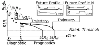
[image:3.612.90.250.242.316.2]The goal of the proposed framework is to estimate the cur-rent transformer insulation health state given inspection data up to now (diagnostics) and predict the likely future remaining lifetime given hypothetical future profiles (prognostics). Fig. 1 shows the PHM analysis framework where{z1,. . . ,zi,. . . ,zk} is the inspection data up to the current time instanttkand EOLi denotes end of life due to to the i-th degradation trajectory.
Fig. 1. Transformer insulation paper PHM framework
The generalization and accuracy of the HST model in (2) can be enhanced by complementing the equation with forecast-ing models. The analytic equations used to quantify ΘTO(t) are not always accurate [10], [14] because it is difficult to generalize with an analytic relation the properties of different transformers operating in different contexts and this affects transformer lifetime estimation. Accordingly, a novel RUL prediction framework is proposed shown in Fig. 2.
Fig. 2. Proposed remaining paper lifetime framework
The inspection data is not directly processable because it may include outliers and noisy measurements. The data preprocessing step denoises and filters the data. Subsequently the segmentation step divides the time series into different equidistant time periods. The preprocessed and segmented data is then connected with a feature extraction step so that a number of time-domain features are extracted. Finally, this stage is completed by selecting the most representative features for subsequent thermal and lifetime modelling steps (see Subsection III-A).
The thermal modelling approach is comprised of top-oil and HST calculations. For a number of utilities it is common not to have HST measurements because the required sensors are not cost-effective. Accordingly, machine learning (ML) techniques have been used to learn a predictive model which is able to predict the top-oil temperature,ΘˆTO, given a number of input parameters (see also Subsection III-B). Then this model is used along with the IEEE experimental model to estimate the HST:
ˆ
ΘH(t) = ˆΘTO(t) + ∆ΘTO,H(t) (8)
The only difference between (8) and (2) is that the TOT is predicted using ML models and not using analytic equations. After implementing the HST prediction model, it is possible to embed it into the lifetime modelling framework through the PF approach for a more accurate lifetime estimation which includes different uncertainty criteria (see Subsection III-C).
A. Data pre-processing & feature selection
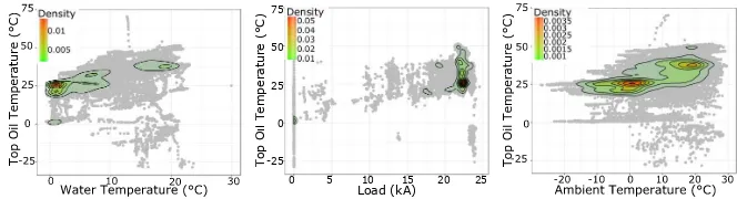
After denoising and filtering the measurements performed on-site (see Section IV), Fig. 3 shows the correlation of the top-oil temperature (vertical axis) with cooling water tempera-ture, load and ambient temperature (horizontal axis), where the grey points are the actual data samples. The higher the density (plotted in red) the more likely is the correlation and vice-versa (plotted in green). For instance, the most likely condition for water temperature versus top-oil temperature (Fig. 3 left) is that for water temperature between 0◦C and 5◦C the top-oil temperature is concentrated at 25◦C with a probability density value of 0.015. As the water temperature increases up to 10◦C, the top-oil temperature fluctuates between 20◦C and 35◦C with a probability density value of 0.001 (green area in Fig. 3 left). It can be seen in Fig. 3 that there is a non-linear relationship among the measured variables and the top-oil temperature. This indicates that these variables may be good predictors for top-oil temperature because they add new information to the forecasting model. This confirms expert knowledge [7] which states that for water-cooled transformers, the relevant parameters to estimate top-oil temperature are cooling water temperature, ambient temperature and load.
In order to improve the prediction capability of forecasting models, it is possible to infer additional time-domain features from water temperature, ambient temperature and load time-series. To this end, first the time series is divided into seg-ments, and then features are inferred. Different state-of-the-art features have been extracted (listed in Table I [25], [26]) which results in a total of 18 features plus the three time series.
TABLE I
TIME-DOMAIN FEATURES OF THEk-TH SEGMENT OF THE INPUT DATA CONTAINING A TOTAL OFNDATA SAMPLES,xi,k,PER SEGMENTk
Feature Definition Feature Definition
Mean X1=ΣNi=1xi,k
N
Impulse
factor X2=
max(|xi,k|) 1
NΣNi=1|xi,k|
Skewness X3= ΣN
i=1(xi,k−µk)3 (N−1)σk3
Kurtosis X4= ΣN
i=1(xi,k−µk)4 (N−1)σk4
Root mean
square X5=
r ΣN
i=1x2i,k N
Crest factor
X6=
max(|xi,k|) r
1
NΣNi=1x2i,k
[image:3.612.312.563.521.590.2]Load (kA)
Top Oil
Tempera
ture (°
C)
0 5 10 15 20 25 0
[image:4.612.137.469.55.145.2]-25 25 50 75
Fig. 3. Top-oil temperature correlated with cooling water temperature, load and ambient temperature
account lagged signals and their effect on the prediction (see LSTM models in Subsection III-B4).
The feature selection process is implemented in Section IV-B1 using the case study datasets. Accordingly, the design of the subsequently introduced machine learning algorithms are based on these datasets and extracted features.
B. Thermal modelling through machine learning methods
So as to forecast the top-oil temperature, different ML models have been designed and tested including Random Forests (RF) [27], Artificial Neural Networks (ANN) [28] and Support Vector Regression (SVR) [29], and also improved versions of RF (Extreme Gradient Boosted Regression Tree, XGB [30]) and ANN (Long Short Term Memory, LSTM [31]). The rationale for choosing these models is to compare the predictive power of XGB and LSTM with their counterpart models (RF, ANN) and other classical models (SVR).
1) Random Forests (RF): RF is an ensemble of recursive trees [27]. Each tree is generated from a bootstrapped sample and a random subset of descriptors is used at the branching of each node in the tree. RF creates a large number of trees by repeatedly resampling training data and averaging differences through voting.
The RF model has been implemented through the
randomForestpackage in R. The hyperparameters include
the number of trees (ntree) and the number of variables randomly sampled as candidates at each split (mtry). These parameters have been optimized through a 10 repeated 5 fold cross-validation (CV) process searching the best parameters from a predefined grid of parameters (see Subsection IV-B2 for more details of the CV process): ntree=[100, 500, 1000, 1500] and mtry=[1:15]. Best results were obtained with ntree=500 and mtry=2.
2) Extreme Gradient Boosted Regression Tree (XGB): XGB [30] is a faster and more efficient implementation of gradient boosting [32] which creates an accurate learner by combining many regression trees. The objective of training an XGB model is to minimize the training loss and avoid overfitting through regularization terms. This process is based on additive training implemented through a second order gradient algorithm [30]. The XGB model has been implemented through the
xgbtree package in R. The hyperparameters include the
maximum depth of the tree (max depth) and learning rate (η). The more complex the tree, the more complicated patterns it will learn, but it will be more prone to over-fitting. The learning rate models the error generalization. These hyper-parameters have been optimized through a 10 repeated
5-fold CV process searching the optimal parameters from a predefined grid of parameters:η=[0.001, 0.003, 0.01, 0.1, 0.3], max depth=[1, 2, 4, 6, 10]. The best parameters for this work areη=0.3 and max depth=2.
3) Artificial Neural Network (ANN): ANNs are widely used for classification and regression tasks [28]. The multilayer perceptron (MLP) feedforward model was used in this work. The MLP is a three-layer network (input, hidden, output) comprised of fully connected neurons. Each neuron performs a weighted sum of its inputs and passes the results through an activation function. All the designed ANN models use a sigmoid activation function for the hidden layer and linear activation function for output nodes.
Model training is performed using a back-propagation al-gorithm. The goal is to learn the neuron weights to generate the network output from the sample input, which minimizes the error with respect to the target output. 10 repeated 5 fold CV was used to select an optimal number of hidden nodes. A number of networks were trained for each fold varying the number of hidden nodes from 1 up to 30. Of the trained networks, the one with the highest accuracy was selected and was comprised of 13 hidden nodes. The ANN was implemented using thennetR package.
4) Long Short Term Memory (LSTM): Is a type of recurrent neural network which can capture correlations among signals which involve long or short term time lags [31]. An LSTM model is comprised of one input layer, one or more recurrent hidden layers, and one output layer. The recurrence loop allows layers to store information. Instead of using nodes for the hidden layer as in ANN models, the basic units of LSTM models are cells, which can perform complex logic operations (sometimes resembling finite state machines). The LSTM model is trained through back-propagation of errors using stochastic gradient descent.
The LSTM model has been implemented through the
Keraspackage in Python. The hyperparameter tuning process
consists of selecting the next parameters: number of layers, number of LSTM units, batch size, learning rate, and number of epochs. Batch size denotes the subset size of the training data. The LSTM model is not trained in a single trial, but takes subsets of the data and learning correlations between subsets. Each batch trains a network in successive order taking into account the updated weights coming from the previous batch. Number of epochs is the number of forward and backward passes of all the training data.
different hyperparameters were tested through 10 repeated 5-fold CV and grid search with parameters defined in the following ranges: batch size = [5, 10, 15, 30, 45, 90], number of cells=[1:30], epochs=[10, 1000, 2000, 4000, 5000, 10000], activation functions = [softmax, relu, linear, tanh, sigmoid, softsign, softplus], learning rate = [1e-4, 1.5e-4, 2e-4, 3e-4, 4e-4, 5e-4, 1e-3, 2e-3]. Best results were obtained with two layers with 7 cells in each layer, batch size of 15, 5000 epochs, learning rate of 1.5e-4 and softmax activation function.
5) Support Vector Regression (SVR): The SVR maps input data into an m-dimensional feature space using a kernel function [29]. The kernel translates a nonlinearly separable problem into a feature space, which is linearly separable by a hyperplane. The SVR defines a ǫ loss function that ignores the errors situated within a certain distance of the true value. The SVR is parametrized through the choice of kernel function. For a nonlinear problem the RBF kernel is recom-mended: k(x, x′) = exp(γ||x−x′||2), where γ is the RBF width, x and x′ are training and testing data samples, and ||d|| is the Euclidean norm. The SVR solves an optimization problem maximizing the distance from the hyperplane to the nearest training point. SVR penalizes the loss function with a cost variable c. SVR training consists of calculating the hyperparameterscandγ. Model training was performed using the R kernlab and MLR packages and grid search was used to optimize c and γ within c = [2−8,2−4,2−2, 1] and γ = [2−8:2:24]. Of the trained SVRs, the one with the highest accuracy was selected which had ǫ=0.1,γ=0.25 andc=1
C. Lifetime modelling through Particle Filtering (PF)
PF is a Monte Carlo based Bayesian filtering method. PF enables the integration of multiple measurements in a single degradation modelf(·)and filters the true state of the system, xt, taking into account multiple sources of uncertainty [33]. A two-step method is implemented when PF is used for PHM [34]. Firstly the system state estimation is performed:
xk=f(xk-1, wk-1) (9)
zk=h(xk, ϕk) (10)
wheref(·)is the state degradation function,wkis a state noise vector wk = hwt, wRULti, h(·) is the measurement function,
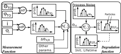
andϕk is a measurement noise vectorϕk=hϕTO, ϕii. Fig. 4 shows the application of (9) and (10) in the trans-former paper RUL estimation process. The measurement func-tion defined in (6) integrates load (i) and top-oil temperature (ΘTO) along with their measurement errors (ϕi and ϕTO) and other transformer parameters, and computes the hot-spot temperatureΘH. The degradation function defined in (7) integrates the process noise Wt and calculates the RUL from the HST and initial health state. The initial health state is then iteratively updated with the actual state.
[image:5.612.337.533.54.142.2]The state estimation xk given measurements zk up to the time instant k is defined in terms of probability density function (PDF) p(xk|z0:k). The initial state p(x0) is assumed to be known (see diagnostics in Fig. 1). There are different methods to estimate the transformer’s initial health state such as the experimental analysis of the degree of polymerization of the insulation paper, or if the paper is new, the initial
Fig. 4. PF framework for transformer insulation paper analysis
health state may be assumed to be of 180000 hours under the conditions stated in IEEE C57.91 [7]. The prior PDF of the state xk from the distributionp(xk-1|z0:k-1) is determined by:
p(xk|z0:k-1) =
Z
p(xk|xk-1, z0:k-1)p(xk-1|z0:k-1)dxk-1
=
Z
p(xk|xk-1)p(xk-1|z0:k-1)dxk-1
(11)
where the state-transition distribution function p(xk|xk-1) is defined by the recurrence relation form in (9). In order to update the prior PDF, a new measurement is collected at time k;zk, and the posterior PDF is obtained using the Bayes rule:
p(xk|z0:k) =
p(xk|z0:k-1)p(zk|xk)
p(zk|z0:k-1)
(12)
The analytic solution of (12) is complex. Thus, the PF was proposed based on iterative application ofprediction,
updateandresamplingsteps at each time instantk[33].
Prediction:assuming at timek−1,Nprandom samples
(particles) of the system state are available, {xi k−1}
Np i=1, as a realization of the posterior distribution p(xk-1|z0:k-1), the prediction at k is performed by sampling the probability distribution of the system noisewk-1and simulating the system dynamics according to (9) to generate new samplesxi
k which are realizations of the predicted distributionp(xk|z0:k-1).
Update: each sampled particle is assigned a weight based
on the likelihoods of observationszk collected at timek:
wi k=
p(zk|xik)
PNp
j=1p(zk|xjk)
(13)
An approximation of the posterior PDF p(xk|z0:k)is then obtained from the weighted samples{xi
k, wik} Np
i=1.
Resampling: as the PF evolves in time, weight
de-generacy phenomena occurs where all but one particle have negligible weights [33]. To avoid this problem a degeneracy condition is defined based on the effective size:
ˆ
Neff= 1/
Np
X
i=1
wik (14)
IfNeffˆ falls below a thresholdNT(NT=Np/2in this work), a systematic resampling step is applied [33].
Algorithm 1 below is a variant of the PF framework and defines the model implemented in this work for transformer paper lifetime modelling as defined in Fig. 2.
IV. CASESTUDY
Algorithm 1 PF framework for paper lifetime prediction
1: {RU Lk-1, xik−1, w
i k−1}
Np
i=1 ⊲Results from instantk−1
2: for k=1:∆t:Pred.Horizon do⊲Iterate∆ttimestep until horizon 3: Read and pre-process measurements
4: Segment data, extract and select features atk:{xk} 5: Forecast ΘHˆ (k) from (8)
6: Sample error variables: rTO∼N( ˆΘTO,ϕTO), ri∼N(i, ϕi),
rRULk-1 ∼N(RU Lk-1, wRULk-1),rk∼N(0, wk)
7: fori= 1 :Np do ⊲Statepredictionstep 8: Propagatexi
k using (9), (10),RU Lk-1 &ΘTO(ˆ k) 9: Compute{wk}i Np
i=1, using (13) ⊲Update
10: ifNˆeff< NT then ⊲Resamplingcf. (14)
11: Updatexi
k andwikvia systematic resampling
12: RU L[k]← {xi k, wik}
Np
i=1 ⊲Store particle results at timek
13: RU Lk-1=RU L[k] ⊲Update for the next iteration 14: returnRU L⊲All particles & weights in the prediction horizon
distribution models the uncertainty-related variables (cf. Algo-rithm 1, line 6). For confidentiality reasons, it is assumed that the initial state of the insulation paper is equal to a new paper with 180000 hours of life and an uncertainty of 500 hours, i.e.RU L0∼N(180000,500)[7] and the process noise is assumed to be rk∼N(0,20). However, note that the PF framework is flexible and it enables the integration of non-Normal distributions too.
TABLE II
TRANSFORMERPARAMETERS
Param. Value Param. Value
Cooling / m,n Oil Directed Water Forced / 1, 1 Rating 267 MVA ∆H,R/∆TO,R 30◦C / 24.3◦C V1/V2 17 kV/230√3kV
wcore,coil/wtank 95254 kg / 30617 kg ir/γ 15.1 kA/0.25
A. Diagnostics & sensitivity analysis
1) Diagnostics: Using the proposed framework in Fig. 2, it is possible to estimate the actual health state of the insulation paper by replacingline 5of Algorithm 1 with realΘTO(t) measurements and scoping the prediction horizon into the length of the available data.
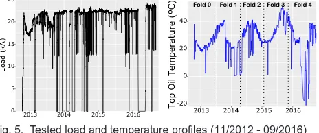
Assuming that the initial health state corresponds to 11/2012 the health state after 3 years and 10 months is evaluated, i.e. at 09/2016. Accordingly, the available datasets for top-oil and load for the same period are processed so as to first calculate the HST [cf. (6)] and then estimate the RUL at 09/2016. Fig. 5 shows the preprocessed load and top-oil temperature data.
Load (kA)
2013 2014 2015 2016 0
[image:6.612.55.301.63.231.2]5 10 15 20 25
Fig. 5. Tested load and temperature profiles (11/2012 - 09/2016)
In order to calculate the health state of the transformer as of 09/2016, it is assumed that the temperature error is ϕTO = 5 ◦C and the load error is ϕi = 1 kA. The datasets in Fig. 5 are applied to the PF framework in Algorithm 1 as follows:
• line 1: initial state: RU L0∼N(180000,500).
• line 5: calculate the HST from (2) using the collected
top-oil temperature data in Fig. 5.
• line 6: draw random numbers corresponding to the
selected error variables.
• lines 7-13: calculate the PDF of the RUL att.
This process is repeated for the selected prediction horizon
(line 2) with a ∆t=1 hour timestep, and finally the PDF
of the RUL is obtained after processing all the available data
(line 14). There is no need to extract features and predict
the TOT because the TOT is available until 09/2016 and the goal is to diagnose the health state at this time instant.
Fig. 6 shows transformer lifetime diagnostics results. The operating time axis denotes the processed data (11/2012-09/2016), the RUL axis denotes the degradation of the health state starting from the initial state, and the density axis denotes the PDF value.
0.002
0.001
0
D
Jul 2016 Jan 2016
Jan 2015 Jan 2014
Jul 2013
Jul 2014
Jul 2015
180k 176k 174k 172k 170k 168k
178k Remaini
ng Useful Li
fe (hours )
[image:6.612.349.521.253.404.2]Operating ti me Jan 2013
[image:6.612.315.561.466.548.2]Fig. 6. Transformer diagnostics results for 11/2012-09/2016
Fig. 7 shows the health state of the transformer at the initial and final time instants directly taken from Fig. 6.
Fig. 7. RUL at initial and final time instants (inferred from Fig. 6)
An important result is that the initial assumptions about the Normal distribution of the errors (cf. Fig. 7 left) change as the PF framework propagates the measurements and associated errors. By the end of the diagnostics process (cf. Fig. 7 right) Normality cannot be assumed and therefore, when inferring the confidence intervals, standard percentile values are not applicable. Namely, the final health state is distributed into two nodes located at 169300 and 170200 hours. Accordingly, it is necessary to calculate the area under the curve so as to ensure that it covers the desired confidence interval (CI) area. Fig. 8 shows the 95% confidence interval quantification concept for non-Normal distributions bounded into [95- CI, 95+CI].
[image:6.612.54.286.582.679.2]Fig. 8. 95% confidence intervals [95-CI, 95+CI]
[image:7.612.358.514.59.203.2]an uncertainty-informed decision with intuitive lower and upper limits on the estimated parameters. Accordingly, Fig. 9 shows the maximum likelihood and 95% CI of the predictions in Fig. 6.
[image:7.612.99.246.199.315.2]Fig. 9. Transformer diagnostics, 95% CI of Fig. 6
Fig. 9 shows the maximum likelihood and 95% CI for the PDFs shown in Fig. 6. The degradation is almost exponential as determined by the ageing acceleration factor in (1), but this is affected by the de-energized periods of the transformer which are reflected in the load and top-oil temperature. For example, the transformer was shut down in mid-2016 which resulted in zero load, decreased top-oil temperature, and accordingly almost negligible RUL decrease. The uncertainty propagation is dependent on the assumed error variables and processed data as discussed in the next subsection.
2) Sensitivity Analysis: In order to evaluate the effect of error variables on the RUL estimation a sensitivity analysis has been performed examining the effect of the change of load and temperature measurement errors. Note that this information is lost with existing lifetime estimation models.
The HST in (6) defines the effect of load and temperature measurements errors. For this case study (cf. Table II), this equation is parametrized as follows (i(t),ϕi are in kA units):
ΘH(t) = ΘTO(t)+ϕTO+ [∆H,R/ir2].[i(t)2+ϕi2+2.i(t).ϕi] = ΘTO(t)+ϕTO+0.13.i(t)2+0.13.ϕi2+0.13.i(t).ϕi
(15)
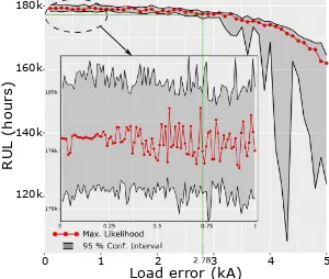
It is possible to see that the effect of temperature measure-ment errors are added as absolute values. In contrast, for small load variations, the effect of load measurement errors on the HST are not relevant. However, ifϕi>p
(1/0.13)∼2.78 then the effect starts increasing rapidly due to the factor 0.13.ϕi2 and the exponential degradation in (7). The term 0.13.i(t).ϕi depends on the specific transformer loading.
The effects of different load and temperature errors have been analysed using monitored data. For computational effi-ciency the data has been limited to a year (11/2012-11/2013). Fig. 10 shows the effect of different load measurement errors on lifetime estimation assuming constant temperature mea-surement error (N(ΘTO,5)) and process noise (N(0,20)).
110k 120k110k130k
140k150k 160k
1k
1k
5 4
3 2
1 0
Load err or (
kA)
R ng Useful Li
fe (hour s) 0
0 00 0 00 0 00
Fig. 10. Load error sensitivity analysis — 3D representation
It is apparent from Fig. 10 that different load measurement errors play a different role on the lifetime estimation. Fig. 11 shows the maximum likelihood and 95% CI for the load error sensitivity analysis inferred from Fig. 10.
Load error (kA)
RUL (hour
s)
180k
9 o !" #$l
160k
140k
120k
0 1 2 3 4 5
17 17 18
2 %&
Fig. 11. Load error sensitivity analysis with 95% CIs
As the load measurement error magnitude increases in Fig. 11, the uncertainty bounds increase and the maximum likelihood value decreases. The zoomed view of the interval [0.01-1] kA shows that the error bounds are around 2000 hours and they are fairly constant in this zone. However, around the elbow point identified in (15) the maximum likelihood value starts decreasing rapidly and the 95% confidence intervals widen due to the increased effect of the error values. Owing to the stochastic nature of the PF algorithm, the 95% CIs vary according to the nature of the PDF (see PDFs in Fig. 10).
In order to evaluate the effect of temperature errors, the load measurement error (N(i(t),1)) and process noise (N(0,20)) have been assumed constants. Fig. 12 shows the 95% CI for effect of error measurements for this situation.
[image:7.612.360.510.306.433.2]Fig. 12. Temperature error sensitivity analysis
On the other hand, above a temperature error of 5◦C the effect of the temperature error becomes non-negligible and it directly affects the health state. Additionally, it is possible to see that for temperature measurement error values below 2◦C the CIs are very narrow, but as the error increases these bounds widen. This is because for low temperature errors the model is confident that the final health state is the maximum likelihood value because there is no temperature error. However, as the temperature error increases, the CIs widen and the final evaluation of the health state is more uncertain.
When the load error is zero and the temperature measure-ment error is 5◦C (Fig. 11) the variation of the RUL estimation is caused by the term ϕTO in (15). In contrast, when the temperature measurement error is zero in Fig 12, but the load error is kept at 1kA, it can be seen that the variation due to the term ϕi in (15) is almost negligible, which confirms that the effect of temperature errors are more sensitive than load errors for low loading conditions.
B. Prognostics
In order to predict the future health state of the transformer the approach shown in Fig. 2 is adopted. First an appropriate predictive model is designed which is able to estimate HST given hypothetical load and temperature profiles. This estima-tion can then be directly connected with the PF framework to propagate uncertainties and estimate the lifetime. The adopted temperature error isϕTO= 5◦C and load errorϕi= 1kA.
1) Feature processing & selection: The length of the segment determines the validity of features and the final prediction error. According to the performed experiments, best results were obtained with a length of 5 days. With a segment length longer than this the features lost representativeness and the error increases (see Fig. 13) .
Subsequently, all the features (cf. Table I) along with the preprocessed variables have been processed through a recursive feature elimination (RFE) procedure and grid search [35]. This step selects the most representative features which minimize the prediction error. RFE was implemented for RF, XGB and SVR using the Caret R package and grid search was implemented for ANN and LSTM models. The error is quantified through 10 repeated 5 fold CV using the normalised root-mean-squared error (RM SE):
RM SE= RM SE max{RM SEi}Ni=1
;RM SE=
v u u t
PN i=1
ˆ ΘTO−ΘTO
2
N (16)
whereN is the number of predicted data samples.
[image:8.612.324.544.117.220.2]Fig. 13 shows the feature selection results with best features for different segment sizes for XGB and RF models. Best results were obtained with the listed 12 features in Fig. 13.
Fig. 13. Feature selection and segment size
Best results for SVR were obtained with three features (water temperature, mean ambient temperature, load), nine for ANN models (water temperature, mean ambient temperature, mean load, RMS water temperature, mean water temperature, skewness water temperature, RMS load, kurtosis ambient tem-perature, IF ambient temperature) and six for LSTM models (water temperature, mean ambient temperature, load, RMS load, mean load, mean water temperature) all with a segment size of 5 days. After the feature extraction step, all the forecasting models have been designed and trained according to the process outlined in Subsections III-B1-III-B5.
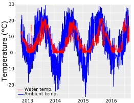
2) Thermal modelling: The first step is to learn a predictive model so as to predict the top-oil temperature. Figs. 5 and 14 show load, ambient, water and top-oil measurements hourly sampled for a period of 3 years and 10 months.
Fig. 14. Water and ambient temperature data (11/2012-09/2016)
It can be seen that the top-oil temperature profile is highly non-linear due to the specific operational constraints of NPPs. Namely, the plant is shut down for maintenance activities and this affects the load and top-oil temperature values. Additionally, depending on the harshness of the winter, load conditions and applied water temperature, the oil temperature can drop below zero degrees, e.g. winter 2016.
[image:8.612.371.502.429.530.2]behaviour of some models and generate repeatable results. For the error calculation the RMSE has been used. Note that there are different alternatives to validate the results such as the stratified double CV scheme [26].
In total, after preprocessing the data and removing invalid samples, there are 32440 samples so each fold has 6488 samples. Accordingly, at each fold the models predict up to 6488 hours ahead (∼271 days). Table III displays the mean RMSE and the standard deviation for various models for all the folds estimated through the 10 repeated 5 fold CV procedure.
TABLE III
RMSEOFMLMODELS FOR TOP-OIL TEMPERATURE FORECASTING
Tech. Fold #1 Fold #2 Fold #3 Fold #4 Average etrain etest etrain etest etrain etest etrain etest etrain etest
XGB 0.37 ± 0.28 4.13 ± 0.37 1.2 ± 0.35 5.07 ± 0.35 2.08 ± 0.13 6.63 ± 0.67 3.04 ± 0.24 9.1 ± 0.15 1.67 ± 1.14 6.23 ± 2.17 LSTM (2L) 1.77 ± 0.05 3.99 ± 0.42 2.45 ± 0.12 4.13 ± 0.3 2.89 ± 0.15 6.85 ± 0.25 4.63 ± 0.28 9.97 ± 0.39 2.94 ± 1.05 6.24 ± 2.43 LSTM (3L) 1.82 ± 0.09 4.31 ± 029 2.43 ± 0.33 4.39 ± 0.24 3.01 ± 0.28 6.67 ± 0.24 4.21 ± 0.6 9.7 ± 0.11 2.87 ± 0.88 6.27 ± 2.19 LSTM (1L) 2 ± 0.17 4.3 ± 0.71 2.52 ± 0.24 4.4 ± 0.49 3.29 ± 0.52 6.9 ± 0.26 4.34 ± 0.67 9.6 ± 0.52 3.05 ± 1.01 6.3 ± 2.5 RF 0.85 ± 0.02 4.23 ± 0.05 0.84 ± 0.01 5.05 ± 0.06 0.91 ± 0.005 6.49 ± 0.001 1.07 ± 0.005 10 ± 0.005 0.92 ± 0.1 6.4 ± 2.55
SVR 1.66 4.9 2.87 4.13 2.38 6.93 3.5 9.76 2.35 ± 0.77 6.43 ± 2.51 ANN 1.12 ± 1.04 5.8 ± 1.6 1.49 ± 0.27 5.47 ± 0.83 2.07 ± 0.14 6.54 ± 0.18 3.43 ± 0.19 11.07 ± 0.93 2.03 ± 1.01 7.22 ± 2.6 IEEE
C57.91 N/A 5 N/A 5.6 N/A 8.6 N/A 12 N/A 7.77
± 3.2
From the prediction results in Table III it can be seen that the XGB predicts best the top-oil temperature value. The mean performance of the LSTM is practically the same, but in the worst case scenario the maximum error is greater than the XGB, i.e. etestXGB = 8.4< etestLSTM=8.67. Additionally, an
important advantage of XGB over LSTM is that XGB models are easier and faster to train and test. Accordingly, the XGB model is used for lifetime modelling and RUL estimation. Fig. 15 shows the last fold prediction for XGB and LSTM, where ground truth denotes the measured top-oil temperature data.
Fig. 15. Top-oil temperature forecasting results for the last fold (see top-oil temperature and folds in Fig. 5)
RF also shows a good performance, but the problem is that RF overfits the model as shown by the low training error. Also note that different trials of SVR models generate same results because of the fixed decision boundaries.
In contrast, the thermal model defined in the IEEE C57.91 standard has the poorest performance and highlights that the
IEEE analytic model may not perform accurately for every transformer operating in different contexts.
3) Lifetime modelling: The lifetime prediction model uses the most accurate thermal model within the framework in Fig. 2. Given hypothetical ambient temperature, load and water temperature variables, first the selected features are inferred (cf. Fig. 13), and then the XGB model predicts the top-oil temperature. Subsequently, the IEEE model is used to estimate the hot-spot temperature from the predicted top-oil temperature, and finally, this is used to predict the paper RUL using the PF framework defined in Algorithm 1.
[image:9.612.338.522.267.367.2]To test the approach with different hypothetical profiles, one year’s worth top-oil and ambient temperature data have been taken from Fig. 14 as a representative reference for yearly temperature patterns. Then user-defined load profiles are used to predict the TOT under different loading conditions. Fig. 16 shows tested load and temperature patterns.
Fig. 16. Tested future load and temperature profiles
These patterns have been repeatedly applied to the PF framework in Algorithm 1 for two different prediction hori-zons of 5 and 10 years:
• line 1: initial state:RU L0∼N(180000,500).
• line 4: infer selected features from load, ambient
tem-perature and water temtem-perature profiles in Fig. 16.
• line 5: using the designed XGB model, first forecast
the TOT and then calculate the HST.
• line 6: draw random numbers corresponding to the
assumed error variables.
• lines 7-13: calculate the PDF of the RUL at time
instantt.
This process is repeated for the selected prediction horizon
(line 2) with a ∆t=1 hour timestep, and finally the PDF
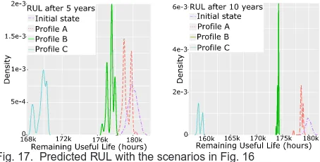
[image:9.612.52.296.563.643.2]of the RUL is obtained after processing the data up until the prediction horizon (line 14). Fig. 17 shows the RUL predictions after 5 and 10 years.
Fig. 17. Predicted RUL with the scenarios in Fig. 16
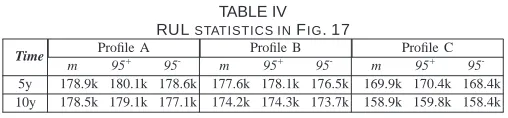
[image:9.612.315.542.591.706.2]TABLE IV RULSTATISTICS INFIG. 17
Time Profile A Profile B Profile C
m 95+ 95- m 95+ 95- m 95+ 95
-5y 178.9k 180.1k 178.6k 177.6k 178.1k 176.5k 169.9k 170.4k 168.4k 10y 178.5k 179.1k 177.1k 174.2k 174.3k 173.7k 158.9k 159.8k 158.4k
The predicted RUL values are consistent with the applied profiles. That is, C shows the most severe degradation followed by B, and the application of A results in a higher RUL.
V. CONCLUSIONS
This paper has presented a novel transformer condition assessment approach integrating model-based experimental models, forecasting models and uncertainty modelling con-cepts in a Bayesian Particle Filtering framework.
Error propagation and sensitivity analysis are key activities for decision-making under uncertainty. The implemented sen-sitivity analysis evaluated the effect of load and temperature measurement errors on transformer lifetime and it showed that for low load measurement errors the effect of temperature errors are more critical. However, the load measurement error increases rapidly above an elbow value which has been formulated analytically.
It has been demonstrated that the integration of machine learning (ML) models with experimental models improves transformer lifetime estimations. Among the tested ML models for thermal modelling, the eXtreme Gradient Boosting (XGB) has shown the best prediction performance. Accordingly, the transformer RUL has been examined with different operational profiles using the XGB-based temperature prediction model, IEEE-based lifetime model and uncertainty information of col-lected measurements and stochastic processes. The predicted RUL values are consistent with the applied operational profiles and this demonstrates the validity of the proposed approach for adaptive lifetime predictions.
As NPPs age, the aging of transformers is becoming increas-ingly critical because they are crucial assets to export energy from the NPP. The proposed approach enables the modelling of these dynamic contexts accurately while accounting for uncertainties. Future work may focus on integrating other degradation accelerating factors in the proposed approach such as the moisture and other chemical factors.
REFERENCES
[1] W. H. Tang and Q. Wu, Condition monitoring and assessment of power
transformers using computational intelligence. Springer, London, 2011.
[2] M. Liserre, G. Buticchi, M. Andresen, G. Carne, L. Costa, and Z. Zou, “The smart transformer: Impact on the electric grid and technology challenges,” IEEE Ind. Electron. Mag., vol. 10, no. 2, pp. 46–58, 2016. [3] H. Ma, T. K. Saha, C. Ekanayake, and D. Martin, “Smart transformer for smart grid - intelligent framework and techniques for power transformer asset management,” IEEE Trans. Smart Grid, vol. 6, no. 2, pp. 1026– 1034, 2015.
[4] J. Aizpurua, V. Catterson, B. Stewart, S. McArthur, B. Lambert, B. Am-pofo, G. Pereira, and J. Cross, “Determining appropriate data analytics for transformer health monitoring,” in NPIC-HMIT, pp. 1–11, 4 2017. [5] M. Djamali and S. Tenbohlen, “Hundred years of experience in the
dynamic thermal modelling of power transformers,” IET Generation,
Transmission Distribution, vol. 11, no. 11, pp. 2731–2739, 2017.
[6] A. Teymouri and B. Vahidi, “Co2/co concentration ratio: A comple-mentary method for determining the degree of polymerization of power transformer paper insulation,” IEEE Elect. Insul. Mag., vol. 33, no. 1, pp. 24–30, 2017.
[7] IEEE PES, “IEEE Guide for Loading Mineral-Oil-Immersed Transform-ers and Step-Voltage Regulators,” IEEE Std. C57.91, 2011.
[8] R. Medina, A. Romero, E. Mombello, and G. Ratta, “Assessing degra-dation of power transformer solid insulation considering thermal stress and moisture variation,” Electr. Pow. Syst. Res., vol. 151, pp. 1–11, 2017. [9] Y. Cui, H. Ma, T. Saha, C. Ekanayake, and D. Martin, “Moisture-dependent thermal modelling of power transformer,” IEEE Trans. Pow.
Del., vol. 31, no. 5, pp. 2140–2150, 2016.
[10] A. Seier, P. D. H. Hines, and J. Frolik, “Data-driven thermal modeling of residential service transformers,” IEEE Trans. Smart Grid, vol. 6, no. 2, pp. 1019–1025, 2015.
[11] E. Pournaras and J. Espejo-Uribe, “Self-repairable smart grids via online coordination of smart transformers,” IEEE Trans. Ind. Infor., vol. 13, no. 4, pp. 1783–1793, 2017.
[12] M. Andresen, V. Raveendran, G. Buticchi, and M. Liserre, “Lifetime-based power routing in parallel converters for smart transformer appli-cation,” IEEE Trans. Ind. Electron., vol. 65, no. 2, pp. 1675–1684, 2018. [13] J. Velasquez, M. Sanz, and S. Galceran, “General asset management model in the context of an electric utility: application to power trans-formers,” Electr. Pow. Syst. Res., vol. 81, no. 11, pp. 2015–2037, 2011. [14] D. Villacci, G. Bontempi, A. Vaccaro, and M. Birattari, “The role of learning methods in the dynamic assessment of power components loading capability,” IEEE Trans. Ind. Electron., vol. 52, no. 1, pp. 280– 290, Feb. 2005.
[15] M. Hell and P. Costa and F. Gomide, “Participatory learning in power transformers thermal modeling,” IEEE Trans. Pow. Del., vol. 23, no. 4, pp. 2058–2067, Oct. 2008.
[16] L. Souza, A. Lemos, W. Caminhas, and W. Boaventura, “Thermal mod-eling of power transformers using evolving fuzzy systems,” Engineering
Applications of Artificial Intelligence, vol. 25, no. 5, pp. 980 – 988, 2012.
[17] A. Bracale, G. Carpinelli, M. Pagano, and P. D. Falco, “A probabilistic approach for forecasting the allowable current of oil-immersed trans-formers,” IEEE Trans. Pow. Del., vol. PP, no. 99, pp. 1–1, 2018. [18] Q. Chen and D. M. Egan, “A bayesian method for transformer life
estimation using perks’ hazard function,” IEEE Trans. Pow. Sys., vol. 21, no. 4, pp. 1954–1965, 2006.
[19] D. Zhou, Z. Wang, and C. Li, “Data requisites for transformer statistical lifetime modelling - part I: Aging-related failures,” IEEE Trans. Pow.
Del., vol. 28, no. 3, pp. 1750–1757, 2013.
[20] E. Chiodo, D. Lauria, F. Mottola, and C. Pisani, “Lifetime characteri-zation via lognormal distribution of transformers in smart grids: Design optimization,” Applied Energy, vol. 177, pp. 127 – 135, 2016. [21] M. Humayun, M. Z. Degefa, A. Safdarian, and M. Lehtonen, “Utilization
improvement of transformers using demand response,” IEEE Trans. Pow.
Del., vol. 30, no. 1, pp. 202–210, 2015.
[22] V. M. Catterson, J. Melone, and M. S. Garcia, “Prognostics of trans-former paper insulation using statistical particle filtering of on-line data,”
IEEE Elect. Insul. Mag., vol. 32, no. 1, pp. 28–33, Jan. 2016.
[23] L. Jauregui-Rivera, X. Mao, and D. Tylavsky, “Improving reliability assessment of transformer thermal top-oil model parameters estimated from measured data,” IEEE Trans. Pow. Del., vol. 24, no. 1, pp. 169–176, 2009.
[24] W. H. Tang, K. Spurgeon, Q. H. Wu, and Z. J. Richardson, “An evidential reasoning approach to transformer condition assessments,” IEEE Trans.
Pow. Del., vol. 19, no. 4, pp. 1696–1703, 2004.
[25] T. W. Rauber, F. Boldt, and F. M. V. ao, “Heterogeneous feature models and feature selection applied to bearing fault diagnosis,” IEEE Trans.
Ind. Electron., vol. 62, no. 1, pp. 637–646, Jan. 2015.
[26] R. Razavi-Far, M. Farajzadeh-Zanjani, and M. Saif, “An integrated class-imbalanced learning scheme for diagnosing bearing defects in induction motors,” IEEE Trans. Ind. Infor., vol. 13, no. 6, pp. 2758–2769, 2017. [27] L. Breiman, “Random forests,” Machine Learning, vol. 45, no. 1, pp.
5–32, Oct. 2001.
[28] M. R. G. Meireles, P. E. M. Almeida, and M. G. Simoes, “A compre-hensive review for industrial applicability of artificial neural networks,”
IEEE Trans. Ind. Electron., vol. 50, no. 3, pp. 585–601, Jun. 2003.
[29] A. J. Smola and B. Sch¨olkopf, “A tutorial on support vector regression,”
Statistics and Computing, vol. 14, no. 3, pp. 199–222, Aug. 2004.
[30] T. Chen and C. Guestrin, “Xgboost: A scalable tree boosting system,” in
Proc. of ACM Knowledge Discov. & Data Mining, pp. 785–794, 2016.
[31] S. Hochreiter and J. Schmidhuber, “Long short-term memory,” Neural
Computation, vol. 9, no. 8, pp. 1735–1780, 1997.
[33] M. S. Arulampalam, S. Maskell, N. Gordon, and T. Clapp, “A tutorial on particle filters for online nonlinear/non-gaussian bayesian tracking,”
IEEE Trans. Signal Process., vol. 50, no. 2, pp. 174–188, Feb. 2002.
[34] B. Saha and K. Goebel, “Model adaptation for prognostics in a particle filtering framework,” Int. J. of Prognostics and Health Management, vol. 2, no. 6, 2011.
[35] M. Kuhn and K. Johnson, An Introduction to Feature Selection, pp. 487–519. New York, NY: Springer New York, 2013.
Jose Ignacio Aizpurua (M’17) is a Research Associate within the Institute for Energy and En-vironment at the University of Strathclyde, Scot-land, UK. He received his Eng., M.Sc., and Ph.D. degrees from Mondragon University (Spain) in 2010, 2012, and 2015 respectively. He was a visiting researcher in the Dependable Systems Research group at the University of Hull (UK) in 2014. His research interests include prognostics and health management, reliability, availability, maintenance and safety (RAMS) analysis and systems engineering for power engineering applications.
Victoria M. Catterson (M’06-SM’12) is a Senior Lecturer within the Institute for Energy and En-vironment at the University of Strathclyde, Scot-land, UK. She received her B.Eng. (Hons) and Ph.D. degrees from the University of Strathclyde in 2003 and 2007 respectively. Her research interests include condition monitoring, diagnos-tics, and prognostics for power engineering ap-plications
Brian G. Stewart (M’08) is is Professor within the Institute of Energy and Environment at the University of Strathclyde, Glasgow, Scotland. He graduated with a BSc (Hons) and PhD from the University of Glasgow in 1981 and 1985 respec-tively. He also graduated with a BD (Hons) in 1994 from the University of Aberdeen, Scotland. His research interests are focused on high volt-age engineering, electrical condition monitoring, insulation diagnostics and communication sys-tems. He is currently an AdCom Member within the IEEE Dielectrics and Electrical Insulation Society.
Stephen D. J. McArthur (M’93-SM’07-F’15) re-ceived the B.Eng. (Hons.) and Ph.D. degrees from the University of Strathclyde, Glasgow, U.K., in 1992 and 1996, respectively. He is a Professor and co-Director of the Institute for Energy and Environment at the University of Strathclyde. His research interests include intel-ligent system applications in power engineering, covering condition monitoring, diagnostics and prognostics, active network management and wider smart grid applications.
Brandon Lambert is a Design Engineering Manager within Bruce Power. He received his B.Eng. degree from Lakehead University, Thun-der Bay, Canada in 2012 and his P.Eng. from the Professional Engineers of Ontario in 2015. His design interests include large power transform-ers, high voltage transmission systems, as well as dielectric and insulating materials.