A study of the brain's transfer function for edge perception

Rochester Institute of Technology

RIT Scholar Works

Theses Thesis/Dissertation Collections

4-7-1987

A study of the brain's transfer function for edge

perception

Charles G. Fink

Follow this and additional works at:http://scholarworks.rit.edu/theses

This Thesis is brought to you for free and open access by the Thesis/Dissertation Collections at RIT Scholar Works. It has been accepted for inclusion in Theses by an authorized administrator of RIT Scholar Works. For more information, please [email protected].

Recommended Citation

A STUDY OF THE BRAIN'S TRANSFER FUNCTION FOR EDGE PERCEPTION

by

Charles G. Fink

A thesis submitted in partial fulfillment of the requirements for the degree

of Master of Science in the Center for Imaging Science in the College of Graphic Arts and Photography of the Rochester Institute of Technology

April 7, 1987

Signature of the Author

Center for Imaging Science

Center for Imaging Science in the College of Graphic Arts and Photography of the Rochester Institute of Technology

April 7, 1987

Signature of the Author

Center for Imaging Science

Accepted by _I

0

Center for Imaging Science

College of Graphic Arts and photography Rochester Institute of Technology

Rochester, New York

CERTIFICATE OF APPROVAL

MASTER OF SCIENCE DEGREE THESIS

The Master of Science Degree Thesis

of Charles G. Fink has been examined and approved by the thesis committee as satisfactory

for the thesis requirements for the Master of Science degree

Dr. Willem Brouwer, Thesis Advisor

Optics Professor, E-O Center, Tufts Institute

The Master of Science Degree Thesis

of Charles G. Fink has been examined and approved by the thesis committee as satisfactory

for the thesis requirements for the Master of Science degree

Dr. Willem Brouwer, Thesis Advisor

Optics Professor, E-O Center, Tufts Institute

Dr. Edward Granger

Image Evaluation Instructor, CIS, RIT

A STUDY OF THE BRAIN'S TRANSFER

FUNCTION FOR EDGE PERCEPTION

by

Charles G. Fink

Submitted to the

Center for _Imaging Science

in partial fulfillment of the requirements

for the Master of Science degree

at the Rochester Institute of _Technology

ABSTRACT

A concept was developed and a computer program was

designed and implemented to model the eye, the _brain, and

the perception system. These models were used to _study

edge transformation through the human visual system. The eye model was developed _using optical spread and neural

sampling data along with different inhibition

distributions. The effects of lateral inhibition on

retinal edge response were studied and hypothetical brain transfer functions were calculated. The results of this

study indicate that no single mechanism or linear model can explain both the sinewave response and edge perception for the human visual system. The eye and brain models were

also used to predict edge perception. The applications and

limitations of computer _modeling are demonstrated for both human vision phenomena as well as artificial vision system

ACKNOWLEDGMENTS

The author wishes to express sincere appreciation to Dr. Willem Brouwer for his encouragement and guidance in the development of this thesis and for the opportunity of being his optics _teaching assistant. Dr. Brouwer s vast knowledge and inspiration was not _only valuable to his students and coworkers but he was also instrumental in restructuring this degree program into what he appropriately named The Center for _Imaging Science_(CIS) .

In addition, the author would like to thank the following people for their valuable assistance and advice:

Dr. Granger of Eastman Kodak Research Labs and _CIS, Dr. Smith, Director Evoked Response _{Lab, Neuro-Opthalmology}, University of Rochester Medical Center and Dr. Williams, Center for Visual _{Sciences, University} of Rochester, for their contribution as thesis committee members and _advising in each of their respective _fields;

TABLE OF CONTENTS

LIST OF TABLES vii

LIST OF FIGURES viii

1. INTRODUCTION 1

1.1 Optical Qualities of the Eye 4

1.2 _{Neurophysiology 5}

1. 3 Psychophysics 15

1.4 Computer _Modeling 18

2. EXPERIMENTAL ₂₅

2. 1 Program Structure 2 5

2. 2 Eye Model 29

2. 3 Perception 3 4

2. 4 Brain Modeling 3 5

2. 5 Sampling 3 7

3. RESULTS ₄0

3.1 Eye Models 4 0

3.2 Brain Models 56

3. 3 Edge Perception 62

4. CONCLUSIONS 68

5. RECOMMENDATIONS FOR FUTURE WORK 71

APPENDIX A Schematic of the Eye and Physical

Statisitics 74

APPENDIX B Pictures; Ramp, Step and Cornsweet

Edges 77

APPENDIX C Visual System _Modeling Program

Menu _Summary 79

APPENDIX D Table 3 : _Summary of Retina Responses

to Edges as a Function of _Changing the

Excitation and Inhibition Ratios 84

APPENDIX E Table 4: _Summary of Retina Responses

to _Ramp Slopes as a Function of _Changing the

Excitation and Inhibition Ratios 86

REFERENCES 88

LIST OF TABLES

Table 1 : Edge Responses for Three Eye Models as a

Function of _{Adding Progressively} More

Inhibition 13

Table 2 : Retinal Edge Response for Three Eye Models... 49

Table 3 : _Summary of Retina Responses to

Edges as a Function of _Changing the

Excitation and Inhibition Ratios 84

Table 4 : _Summary of Retina Responses to

Ramp Slopes as a Function of _Changing

Figure 1 :

Figure 2 :

Figure 3 :

Figure 4 :

Figure 5 :

Figure 6 :

Figure 7 :

Figure 8 :

Figure 9 :

Figure 10 Figure 11 Figure 12 Figure 13 Figure 14 Figure 15 Figure 16 Figure 17 Figure 18 Figure 19

Figure 20

Figure 21

Figure 22

LIST OF FIGURES

Lateral Inhibition Schematic 7

Lateral Neural Interaction 9

Eye Model Components and _Resulting

Retinal Spread Function 11

Ramp Object and Mach Band Perception 16

Step, Cornsweet Edge and _Resulting

Perceptions 17

Box Diagram of Models 18

Box Diagram of Components 2 3

Schematic of Model Components 2 6

Optical Spread at the Retina Surface 3 0

Brain Transfer Function Calculation 35

Adding Spread and Inhibition Functions.... 41

Eye Models as a Function of Inhibition

Shape 43

Eye Models for Gaus and Wider Gaus

Inhibition 45

Eye Models for Combination Inhibition 4 6

Three Eye Models 4 7

Edges and _{Corresponding} Retina Responses

for _Increasing Cornsweet _Decay Rates 52

Brain Models as a Function of Objects 56

Brain Models Before and After _Scaling 57

Brain Models as a Function of Eye Models.. 59

Eye and Brain Models for Combination 60

Predicted Perception 63

Predicted Perception as a Function of

SECTION I

INTRODUCTION

This _study of the brain's transfer function for edge

perception investigates how edges are transformed through

the visual system. In order to understand the brain's

function in contour _perception, we must first model how an

object is _optically transformed _by the eye and encoded _by

the retina. These retinal signals are then transmitted to

higher order processors in the brain _resulting in the

perception of the object. The _brain, which will be treated

as a "black box"

, will bridge the gap between the encoded

retinal image and _resulting perception.

It is proposed that if one studies _only a limited

region of perception _phenomena, sets certain conditions and

makes some fundamental _assumptions, that linear systems

techniques can then be applied to _modeling the human visual

system. As a result a model can be developed and a

computer program can be written to _study the effects of

lateral inhibition on edge perception.

The initial conditions and assumptions which allow

linear systems _modeling of the human visual system will be

briefly outlined. _{First, only} the foveal region will be

modeled and the same average object luminance will be

also be limited to the perception of _only monochrome _edges,

which are constant with respect to time and stationary in

object space. It is assumed that under these limited

conditions, an eye model _{incorporating} the optical spread,

receptor _sampling and one channel of lateral inhibition in

the retina will model the eye's _primary function in edge

perception. _Finally, it is assumed that this single

channel out of the retina is the _only signal into the brain

model to yield the final perception.

This _study involves four major scientific disciplines.

First, optical science will provide the tools to determine

the optical spread function of the eye. Human visual

system _{neurophysiology} will provide the background for the

image _encoding mechanisms in the retina. Psychophysics

will provide the perception information. _Finally, math

modeling, Fourier transforms and convolutions will be

applied in a computer simulation to analyze how edges are

transformed through the visual system and to calculate the

transfer functions for edge perception.

In order to _apply the convolution _integral, we must

assume that the system is linear and shift invariant.

However, the human visual system is neither linear nor

shift invariant over the perceptible luminance range.

Therefore, the _study will be limited to a region where the

visual system is approximately linear and a transfer

The psychophysical data will be from experiments v/ith

tightly controlled _viewing conditions. For instance, the

objects will be constant with respect to time to minimize

potential transient effects. The edges will be stationary

in object space to minimize _tracking and motion effects.

However, since the human eye is _constantly moving, the term

"stationary" _is

used relative to the object space not the

retinal image. The perception of scenes and recognition of

objects is _extremely complex. To _simplify this process

only edges will be studied with this model.

One of the main goals of this _study is to better

understand possible visual processes and their effect on

edge perception. _However, the _study will also have direct

application to the development of artificial vision systems

and _integrating optics and "smart sensors"

which

incorporate some degree of focal plane signal

1. 1 Optical Qualities of the Eve

The light from an object passes through the cornea,

aqueous _{humor, lens,} and vitreous humor of the eye before

reaching the retina. Due to the _geometry of the _eye, the

light must also traverse through the neurons of the retina

before _reaching the receptors (See Appendix A for details

on the _geometry of the human _eye) .

The spread of light in an optical system can be

measured and used to determine the point spread function.

Briefly, the point spread function describes the energy

distribution in the image of a point source after an

optical _system, in this case the eye. The research of

R. W. Gubisch has developed a function which

approximates the light distribution at the retina surface

for various pupil sizes.

This information can be used to model the _intensity

distribution of a given object at the retina surface. In

order to get the _intensity distribution at the retina

receptors, the light spread due to retinal scatter should

also be considered. In the computer _model, the receptor

signal is represented _by an area of positive response which

will be combined with the negative response due to the

1. 2

Neurophysiology

Neurophysiology provides the retinal signal processing

data. The goal is to use this information to model the

primary function of retinal image preprocessing. The

initial models were based on lateral inhibition, receptor

sampling data and possible neural _intensity nonlinearities.

The receptors in the _retina, the cones and _rods,

convert light _energy into neural signals which are then

processed _by subsequent retina layers. When light is

incident on a receptor a visual pigment is degenerated and

neural signals are transmitted. The research of

Enroth-Cugell ' and Robson2 indicates that there are linear

and nonlinear channels in the cat _retina, therefore neural

nonlinearities must also be considered.

Since the receptors are individual sensors, this is the

point where the retinal image is _discretely sampled. The

retina contains rods that respond to all visible light and

cones which have a response that is a function of the

spectral region. The fovea is a region which contains the

highest _density of receptors and therefore is the _primary

area for edge perception. The fovea receptors are small

cones which have approximately a 30 arc-second

center-to-center separation3'4. This provides a _sampling rate of

The _study of the retina's multi-layered neural network

will be important in _{understanding} how images are _initially

encoded and sent to higher order processors. In the last

twenty years, microelectrode _{sensing technology} developed

an _ability to _directly measure the electrical potential of

cells and provides some of the _preliminary data and

understanding of the possible retinal mechanisms and neural

interactions. Since the human eye can not be probed with

microelectrodes, scientists have measured the neural

interaction of mammals which have a retinal structure

similar to the human eye.

The horseshoe crab, Limulus, is often used in retina

research. The compound eye of the Limulus is _relatively

large which makes it _{very easy} to _directly measure the

response of single cells to a given stimuli. The Limulus

retina is a three dimensional neural network that exhibits

a local _excitatory and extended _inhibitory response5,6.

This type of lateral inhibition mechanism is often used to

-j explain Mach bands and other contrast phenomena .

These _{Electrophysiology} experiments appear to have

confirmed _early lateral inhibition hypotheses and have lead

to new discoveries of cell responses. The research of

Hartline et al8'9

on the simultaneous neural output of

two or more optic nerve fibers has lead to the measurement

of the lateral inhibition of nerve impulses as well as the

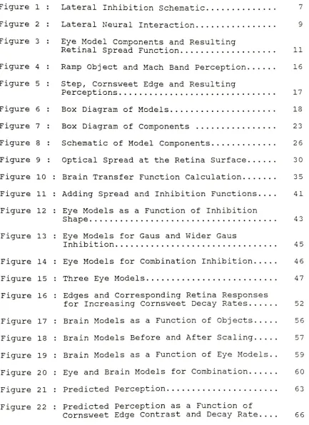
Lateral _{inhibition is}

a _{decrease in the}

signal out of

one cell due to the _{excitation of}

a _{neighboring cell. The}

degree of _{modulation is}

a _{function of}

both cells separation

and _the

intensity

through this

horizontal _{communication}

that _{neighboring cells}

can

influence the _{output of cells}

in other areas of the retina. Figure 1

schematically shows how an edge might be encoded

using a _{very simple}

inhibition model. -1 1.0 OBJECT COMPONENT (""RESPONSE 0.0 0.5 \|/ -1 TOTAL A B C D E F G H B 0.0 0.0 0.0 0.0 0.0 0.0 0.0 -.5 0.0 1.0 -.5

-1 2.0 -1 -1 _2.0 -1 1.0 G H -1 2.0 -1 -1 2.0 0.0 0.0 0.0 0.5 0.0 0.0

SYSTEM RESPONSE

~h>

Lateral _{Inhibition Schematic.}

The response of a _simple

inhibitory

The disinhibition phenomena is a decrease or possible

elimination of _{the inhibition effect}

by receptors

surrounding the _{inhibiting receptors. This} phenomena is

due to an area of _{illumination positioned such} that the

lateral inhibition decreases the signal of the cells which

were _{originally inhibiting the measured cell. As a}

result, this decreases the _inhibiting cells _ability to inhibit.

The net effect is an _increase in the signal of the measured

cell due to the cells _causing disinhibition. This

disinhibition phenomena has also been observed in the human

visual system11.

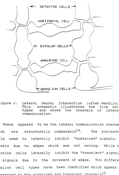
Photomicrographs and _{Electrophysiology} experiments have

lead to the _discovery of five basic types of _cells,

schematically shown in Figure _2, which are arranged in

three distinct layers12. Werblin measured the cell

potentials of the _mudpuppy (Necturus _maculosus) with a fine

micropipette electrode _allowing him to measure the

electrical characteristics of each cell in the retina _using

dye-injection for measured cell identification13. This

data _along with electron micrographs can be used to

schematically diagram the communication channels in the

Figure 2. Lateral Neural Interaction (after Werblin).

This schematic illustrates the five cell

types and shows two channels of lateral

communication.

There appears to be two lateral communication channels

which are _structurally comparable14. The horizontal

cells seem to _laterally inhibit "sustained"

signals, or

signals due to edges which are not moving. While the

amacrine cells _laterally inhibit the "transient" _signals,

or signals due to the movement of edges. Two different

ganglion cell types have been identified which appear to

The research of _{Enroth-Cugell} and Robson support the

idea of two distinct retinal output channels at the

ganglion level of the cat _retina, which _they labeled X and

Y16. Hochstein and _Shapley have suggested that the Y

channel contains a linear excitation _center, a linear

inhibitory surround and _overlapping nonlinear _excitatory

subunits17'18. The experiments of _Devalois, which

studied the response of single cells in the lateral

geniculate nucleus of the Macaque _monkey, discovered that

the non-opponent _excitatory cells _{carry luminosity}

information while the opponent cells do not19.

In addition to at least two different output channels,

the retinal cells have a unique neural response and

architecture with potential perception _{preprocessing} and

detection functions. One lateral inhibition channel will

be considered and _{only stationary} edges will be _studied,

since this computer simulation has one input and one output

channel.

For the computer model let us assume that on the

average the inhibition acts as a linear region of negative

signals _surrounding the input signal, as shown in the

bottom function in Figure 3. If we now add the _excitatory

signal after the optical spread of the _eye, as shown in the

top function, the result is a neural response as a function

RETINA SPREAD FUNCTION COMPONENTS

OPTICAL, OfHlBmjRr <*RESULTANT

a

1

I

OPTICAL

DISTANCE _(ARC-UIN)

INHIBITORY RESULTANT

Figure 3. Eye Model Components _and

Resulting Retinal Spread Function. The spread function shown

was determined _{by adding} the optical and

inhibitory functions.

The _magnitude, shape and spatial extent of neural

inhibition are the main variables in the eye models. The

changes in the shape and spatial extent represent changes

in the strength of the inhibition as a function of distance

from the _neighboring cell to the input _excitatory signal.

Another important variable is the ratio between the

excitation and inhibition areas which represent the

retina's _ability to send _intensity information. These

variables will allow us to _study some of the possible forms

Table 1 shows the shapes of three edges after passing

through the three eye models shown at the _top of each

column (More complete tables can be found in Appendices D

and _E) . The difference in the three _models is due to the

change in the area of the inhibition function. The first

column shows the effects of the optical spread only. In

the second column an area of inhibition is added which has

less area than the excitation. In the final column the

area of inhibition is increased to equal the area of excitation. The first column represents the effect of a

smoothing function and models the appearance of the object at the retinal receptors. The middle retina model is an edge detector which also carries _intensity information.

The retinal response in the last column reflects an edge

detecting mechanism, i.e. the only output signal is due to

a detected change in the object. _Therefore, this model does not _{carry intensity} information.

The recent research of Cornsweet et al presents the

idea of retina _intensity dependent summation . This

concept has also been included as a subroutine in the

computer simulation to allow this option to be compared and

contrasted with inhibition mechanisms.

The multi-layered neural _processing of the retina is

complex and is _likely to contain the first steps of the

pattern recognition process. The fact that the eye "grows"

Table 1. Edge Responses for Three Eye Models as a

Function of _{Adding Progressively} More

it is so difficult to isolate the mechanisms of the eye and

the brain. It also emphasizes how the eye is essentially

an extension of the brain. Since the optic nerve is a

tangible _connecting nerve cord and some ganglion response

data has been documented in other _animals, this is where

the two systems were separated into retinal encoded images

and perceived images.

The encoded retinal images are sent to higher-order

neural networks in the perception process. This visual

information is first processed in the Lateral Geniculate

Nucleus and then the perceptual process is completed at the

Primary Visual Cortex. All of this post retinal image

processing will be incorporated in a black _box, which will

be labeled the "brain".

The brain also appears to be a multi-layered neural

processor. The nobel prize _winning research of Hubel and

Wiesel has lead to considerable progress in the _mapping of

o-i

the macaque monkey's _Primary Visual Cortex . Hubel and

Wiesel have detected _cells, which _they call "simple _cells",

in the higher-order processors which respond best to

certain types of stimuli. These simple cells seem to feed

more complex cells which gives one the idea that there is

some sort of _hierarchy of layers which gets more complex at

each step. Bela Julesz distinguishes two parallel

channels, the preattentive and attentive which also implies

These theories about possible brain mechanisms will be

helpful in _{understanding the} functions of higher-order

processors of visual _{information. These} theories will also

help in _{understanding} how the brain might convert retinal

signals into perceived images and assist in the

interpretation of the _resulting brain transfer functions.

1. 3 Psychophysics

Once eye models have been developed a _variety of object

intensity profiles can be transformed into encoded images.

Next, we need to _apply psychophysics data or models in

order to determine the perception of these edges. This

section will discuss some important edge perception

characteristics and their application in _calculating the

brain's transfer function.

As emphasized in earlier sections the human visual

system is nonlinear and complex, especially when

recognizing objects within scenes. _However, in this _study

we will avoid most of these complexities _{by considering}

only edge perception. To minimize intensity nonlinearities

and eliminate pupil size effects, the objects will differ

only in intensity distribution, not absolute luminance. Therefore the object profiles will have the same average

There have been _many studies in contrast perception of

the human visual system23-34. It is of particular

interest to _study the perception of the ramp, step,

Cornsweet and O'Brien edges. The results of Jeff Pelz's

Masters _Thesis, which studied the induced contrast of the

Cornsweet edge versus the _step35, will also provide an

important source of perception data. Let us begin _by

looking at the Mach band phenomena.

The perception of Mach bands is the result of a _ramp

edge, as shown in Figure 4. The appearance of Mach bands

at the high and low contours of the _ramp is often used to

illustrate the result of a system with an _inhibitory

surround. Note that there is a difference in the shape of

the Mach bands at the high contour versus in the low

contour. This is a type of _nonlinearity in the visual

system which can't be modeled with a simple linear

model36

(Reference Table ₁₎ . A photograph of a _ramp

intensity profile has been included in Appendix B, page _77,

to demonstrate the Mach band phenomena.

OBJECT PERCEPTION

Figure 4. Ramp Object and Mach Band Perception. This

figure shows the intensity profiles of the

The _step and the Cornsweet edge have dramatically different _intensity profiles. However the resulting

perception for both objects is a _step (for limited

contrasts), as illustrated in Figure 5. This is apparently due to the _inability of the human visual system to detect

gradual changes in the Cornsweet edge and therefore only the _step portion is perceived. This will yield important

clues to the low _frequency response of the visual system.

It miqht also _help determine if local retinal processes

carry intensity information (See Appendix _B, page _77, for

pictures of the Cornsweet _illusion) .

OBJECT PERCEPTION

STEP >

CORNSWEET

EDGE

t>

Figure 5 Step, Cornsweet Edge and _Resulting Perceptions. This figure illustrates that the perception of

1-4 Computer _Modeling

Once we have _information about the retinal output and

the _{resulting perception, we will have the response of one}

component and the system response. We can treat these

systems as "black boxes" _to

graphically show the goals of

this _study, as shown in Figure 6.

object _{(x) -y\}

Retina

sr(x)

--> Retinal Response(x)

object _(x) >

Human Visual System

Retina

sr(x)

Brain

sb(x)

-^Perception _(x)

Figure 6. Box Diagram of Models.

(sr(x) and _SjD(x) represent each "black box" _in

spatial _domain, for the retina and brain respectively. ₎

The goal is to model the retina and then solve for the

"brain black box"

. In this paper the

"brain" _is

any post

retinal signal processing. We will also assume that the

lateral inhibition channel out of the retina. In order to

obtain the transfer function for the _brain, let us first

review some basic transfer function evaluation techniques.

The convolution _integral, optical spread functions, and

Fourier analysis will be applied to _study the

transformation of edges through the visual system and

calculate the transfer functions. Briefly, the spread

function is a mathematical representation of how a delta

function, or an _infinitely small point _source, will spread

when transformed through a system. The spread function can

then be multiplied point _by point with the object using the

convolution integral (also known as the superposition

3 7

integral ₎ shown in Equation 1.

i(x) =

o(x) * s(x) =

/o(x')

s(x-x') dx' (Equ. 1)

(Where * represents the convolution process

and ' represents the multiplication _process.)

This technique allows the image of an object to be

determined mathematically. _However, in order to _apply this

convolution integral we need a linear shift invariant

system _(L.S.I.) . This is true for modeling many artificial

vision _systems, but may have limited application in human

vision studies. It is assumed that within a limited region

we can represent the optical spread and lateral inhibition

and, _therefore, the convolution integral can be applied.

For a given _input

(object(x)), the output ₍image_(x))

can be determined _{by convolving the} object and the system

spread function in the spatial _domain, shown in Equation 2.

image(x) =

object(x) * spread(x) (Equ. ₂₎

For _example, when the edges in Appendices D and E are

convolved with the models at the _top of each column the

results are the retinal responses (which can also be

considered _images) that fill the _body of the tables.

The Fourier transform allows one to transform from the

spatial domain to a _frequency domain representation. Let

us look at the Fourier transform of the spread function

from spatial domain to _frequency domain.

S(f)

~~^

Spread(x) (Equ. ₃₎

Where represents the Fourier transform and can

be expressed mathematically with the _following Fourier

integral38, shown in Equation 4:

S(f) =

J

e~l27T fx

dx (Equ. ₄₎

Similarly, image _(x) and object_(x) can be represented in the

The inverse Fourier transform _integral, as shown in

Equation _5, allows one to transform back to the spatial

domain:

+00

s(x) =

ys(f)

df (Equ. ₅₎

- 00

The _{frequency representation of the spread function,}

s(x), is called the transfer _function, S(f). The transfer

function describes the optical performance as a function of

frequency components. The transfer function for a perfect

system, for which all frequencies are reproduced _perfectly,

would therefore be a constant equal to one. _However, this

is impossible for natural systems.

The convolution _process, Equation _2, in spatial domain

can also be performed as a multiplication in the _frequency

domain.

IMAGE(f) =

OBJECT(f) * S(f) (Equ. ₆₎

Since this is a point _by point _{multiplication,} it is much

faster than the convolution integral and _especially

efficient for large arrays. Another important advantage of

using the frequency domain representation is that we can

divide the output _by the input. In this case the image can

be divided _by the object, yielding the system transfer

By dividing both sides of Equation 6 _by the object_(f) we

obtain:

IMAGE _(f)

S(f) = _(Equ.

7)

OBJECT _(f)

If we now back-trans form to the spatial domain we have

calculated the spread function for the system.

The Fourier transform will be performed _usinq a

discrete Fast Fourier _{Transf orm(FFT)} 39 . The FFT is an

algorithm which allows a computer program to _efficiently

transform discrete data. Since the retinal receptors are

individual cells, the continuous _intensity distribution at

the retina surface is _discretely sampled at this point.

This receptor _sampling will be represented _{by using} object

arrays with the appropriate number of data points for the

receptor separation. The _sampling rates will be discussed

in more detail in Section 2.5.

The spread function and transfer function _relationship

is _very important. We have seen from Equation 4 that we

can transform the spread function and obtain the transfer

function. _Taking the modulus of _S(f) will give us the

modulation transfer function _(MTF) , which is commonly used

to _specify the _frequency response of an _imaqing system.

follows for sinewave testing:

x(f)max ~

KfJnin

MTF(f) =

(Equ. ₈₎

I(f)max + _Kf) mm

(Where _I(f)Inax and

I(f)min are the maximum and minimum measured _intensity values _{respectively.)}

If the retinal output and final perception for a

certain stimulus are _known, this would allow the transfer

function to be calculated for the retina and for the entire

visual system for that stimulus40.

SR(f) =

Retinal Response_(f)

Object_(f)

(Equ. ₉₎

Sp(f) =

Perception_(f)

Object_(f)

(Equ. ₁₀₎

(Where

SR and

Sp represent the retina and perception modulation transfer functions _{respectively.)}

At this point we assume that the retina and brain

components are linear shift invariant and can be cascaded

to yield the _perception, p(x), schematically shown below:

o(x)

'"Brain"

>r.r. _(x) -9*

sb(x)

->P(x)

Figure 7. Box Diagram of Components. Where _o(x) represents

the _object, r.r.(x) the retinal response to the

These cascaded L.S.I. systems can be convolved to yield

the system _response41, as shown in Equation 11:

sp(x) =

sr(x) *

sb(x) (Equ. ₁₁₎

(Where the subscripts _{p, r,} and b represent

the _perception, retina and _{brain, respectively.)}

In a system with cascaded _components, the convolution of

the spread functions determines the system spread function

(the component transfer functions can be multiplied in

frequency domain) . The brain transfer function can also be

calculated in _{frequency domain, by dividing} the perception

transfer function _by the retina transfer function:

sP(f)

SB(f) = _(Equ.

12)

SR(f)

The computer model will also allow an _object,

perception and eye model to be specified and the _resulting

brain transfer function to be calculated. Once a brain

transfer function is calculated it can be used to "predict

perception". If the eye and brain models are held

constant, the system output can be calculated as a function

of input object. For a linear system, only one model is

required to determine the output for all inputs. However

if the system is not _linear, the models will change as a

SECTION II

EXPERIMENTAL

This section will present the implementation of visual

system _modeling concepts discussed in the introduction.

The emphasis will be on _modeling the physical phenomena of

a visual system. The models were then used to _develop a

computer program to assist in _studying how edges are

transformed through vision _systems, with specific

references to the human visual system and applications to

artificial vision systems. The unknowns in this _study are

the retinal response and the brain's transfer function.

2. 1 Program Structure

It was proposed that if the retinal response can be

approximated, the brain transfer function can be studied as

a function of the edge objects. This study would require

that an edge profile and the _resulting perception are

known. If so, we can then use the optical _spread, neural

sampling and neural inhibition models to compute the

retinal response. The "brain" would then be the black box

linking the retinal response and the final perception.

Figure 8 _{schematically} illustrates the important elements

OBJECT EYE IMAGE

"BRAIN*

BLACK

BOX

OBJECT * (SPREAD+SAMPLING+INHIBITION) ^ B. B -^ IMAGE

Figure 8. Schematic of Model Components.

In order to accomplish these _objectives, the vision model

was split into five major groups: the _object, eye _model,

brain _model, perception model and perceived image.

The program structure was developed to have general

application in _studying a wide _variety of _imaging systems

and to be _directly applied to _developing artificial vision

systems. These _imaging systems could consist of an optical

component, a discrete sampling function and image plane

preprocessing. The program structure and flow of

information were designed with maximum _flexibility to

accommodate both changes _during development and future

expansions into a more complex _modeling tool. Appendix C

The implementation of the structure began with writing

the menus and _{breaking the program into} logical levels.

The _primary functions were defined and an outline was

developed. Then the lowest level functions and _utility

routines were _{identified. These routines were set up} with

generic arrays _{named, function,} modifier and _result, so

that _{any calling} routine would determine which order the

data would fill these arrays. The middle structure could

then be shifted and changed to adapt to program

developments.

Next the arrays were defined and the flow of

information was developed. These arrays were defined so

the data at each of the important stages would remain

unaltered _by subsequent processing. The arrays were:

object, image at the retinal receptors (after the optical

spread) , retina response after the eye (after neural

processing) and the perceived image. The models were

similarly set _up in independent arrays: the optical spread

and inhibition _functions, the eye _model, the brain model

and the perception model.

The arrays all contained 512 elements with the middle

256 points _containing all the information and the 128

points on each end of the _array for the FFT process. The

objects and images are _relatively large compared to the

optical spread and neural processing, therefore these

varied _up to 128 points. For _instance, the retinal model

default value is 12 8 points. _Therefore, when _convolving

the eye model across an edge this is equivalent to passing

a 128 point kernel across a 512 point object. This can be

understood _{by taking Equation 1} and _integrating from -64

to 64 for _every x from -255 to _256, as shown in Equation

13. The object arrays are defined so that all the

information is contained in the middle 256 points within

the 512 point _array which avoids edge problems when

convolving the eye model across the object.

64

i(x) =

o(x) * s(x) =__/o'(x)

'

s(x-x') dx' (Equ. 13)

-64

There are two types of objects: asymmetric and

symmetric _intensity profiles. The asymmetric functions can

be bigger and allow a closer look at changes in the image

at each stage. The symmetric functions have the advantage

2.2 Eve Model

In order to solve for the unknown retinal response, we

must _develop a model of the eye. The region of the visual

system was restricted _{by limiting} the _viewing conditions

and _{by making} a few fundamental assumptions to allow simple

linear models to be developed. The model was first limited

to the foveal region and _{only monochrome, stationary} and

time constant objects were studied. The average luminance

was constant to avoid changes due to pupil changes (e. g.

changes in optical _spread) and other neural nonlinearities

over magnitudes of luminance changes. (Note the phrase

"Eye Model"

refers to the combination of the optics and

neural mechanism and that the signal out of the eye is

referred to as the "retinal _response", so in some cases the

two are _synonymous) .

The object, a one dimensional _{intensity profile,} is

first blurred _by the optics of the eye and the neural

scatter. Light propagates through the _cornea, aqueous

humor, lens, vitreous humor and retinal neurons before the

receptors transform the light _energy into neural signals

(Reference Appendix _A) . In the foveal region, the retinal

neurons are "pulled" away so that this area is thinner than

any other portion of the retina, therefore causing minimal

light scatter. _Assuming that this scatter in the fovea was

eye, we can use the equation developed _by G. Westheimer

(shown in Equation ₁₄₎ which models42

the data of R. W.

Gubisch43. This equation approximates the light

intensity distribution at the retinal surface. Equation 14

is normalized to _unity at the origin and the components and

the resultant are shown in Figure 9 in both spatial and

frequency domain.

f(x) =

0.47exp(-3.3x2) + 0. 53exp(-0. 93 | x| ) (Equ. 14)

Where x is retinal distance in arc minutes.

OPTICAL SPREAD FUNCTION OPTICAL TRANSFER FUNCTION

o. Q.a 0.7 0.0 0.1 0.4 O.J 0.2 0.1 0

-0.1 -0.2 -0.3 -0.4 -OS

-0.0 nininnnnnii Ml) DIM1 1 1 1 1 11 1 III 1 1 11 1 II 1 11 1>IM 1 1 1 1 1 11n1 11

-10 0

DISTANCE(JJIC-UIH)

iiiiniil ImhimnullMiiiiimiiimi uiinuniiiiuiumiiiimim ii n ii miiiimh in

rrutqUMtJCY(CYOJ3/DMGRXK)

Figure 9. Optical Spread Function at the Retina Surface.

Graphical representation of Equation 14 in

spatial and _frequency domain; the _resultant, f_(x) , is the sum of a Gaus and exponential

appropriately scaled to approximate the light

Since the retinal receptors are individual cells, the

retinal image must be _discretely sampled. The fovea is the

region of the retina where the high _frequency perception is

performed and is therefore crucial in edge perception. The

cones in the fovea are _{approximately} 0.5 arc-minutes in

size. The program default value of 0.3125

arc-minutes/sample was chosen to approximate the retinal

sampling rate and coordinate with the _{resulting frequency}

domain (See Section 2.5 for more details).

After the optical _blur, the light _energy is converted

to neural signals and is processed _by the subsequent

retinal layers. This post receptor neural _{processing by}

the _{horizontal, bipolar,} amacrine and ganglion cells

results in at least two distinct signals to the optic

nerve. The current computer model was used to _study the

effects of one channel of neural preprocessing. It was

proposed that _limiting the perception region will allow one

linear function to _{approximately} model the retina's

response to edge stimuli.

If we _say that the neural inhibition on the average can

be approximated _by a symmetric _shape, we can generate

functions to describe this process. _Keeping the optical

spread model constant, it was possible to _study the effects

of _changing the shape and spatial extent of the neural

inhibition. If we hold the object and _resulting perception

inhibition models and the _resulting changes in the "brain"

model. There are four basic neural inhibition equations

available;

-A + a*x (Equ. ₁₅₎

-A-exp(-a'x2) (Equ. 16)

-A*exp(-a-|x| ) (Equ. ₁₇₎

-A'x4+B'

|x| 3+C*x2+D' |x|+E (Equ. ₁₃₎

(Where the capital letters are variables to change the

magnitude and "a" sets the _decay rate and all equations

are a function of retinal _{distance, "x".)}

There is also the _ability to use _any combination of the

above equations. _Noticing that Equations 16 and 17

approach zero _slowly, the program was modified to allow the

user to shift the neural model to go to zero in the

designated eye model window. The result was an _ability to

generate areas of negative _response, or _inhibition, of

different magnitudes as a function of spatial extent. To

avoid negative average signal intensities, it is _necessary

to have the total area of the retinal response equal to or

The program has the _ability to allow nonlinearities in

addition to simple linear models. The three points where

nonlinearities could be applied are before the receptors,

at the receptors transduction of light into neural signals

and after retinal neural processing. One example of a

nonlinear equation option is shown _below;

In Out =

(Equ. ₁₉₎

In+k

where k is a constant. When k is positive the equation

takes the form of a decelerated nonlinear transformation

and when k is negative the _nonlinearity becomes

accelerated.

The optical spread and the neural _processing are

combined to complete the model of the eye. For the simple

linear _model, the spread function and the inhibition are

added. When the nonlinear options are used, more complex

combining techniques are required _depending on where the

2. 3 Perception

The perception options allow the user to generate an

image, directly input perception data or use a perception

model to _{mathematically determine} the image. The user can

define a linear model _using the _existing equations or

insert a new model. The current _models, shown in Equations

20 and _21, were developed _by the research of D. H.

Kelly . Variables _{are used where possible} to _allow the

user to _modify these functions.

f2 .

e{ B f} _(Equ.

20)

C *

(1 + A _f2) * e<"B

*

f> _{(Equ. 21)}

Note that these models are defined in _frequency space and

therefore the equations are a function of frequency. If

the user opts to input perception data _manually, the

program will also allow the calculation of the

corresponding perception transfer function (as shown in

Equation ₁₀₎ .

This _study concentrates on the perception of three

basic edqes; the step, the Cornsweet edge and the ramp.

The Cornsweet versus _step perception data is based on

experiments performed using a Dianza _display system

This system was used to investigate the effectiveness of

the Cornsweet illusion and as a result it can be

confidently stated that within a limited contrast range a

Cornsweet edge can't be distinguished from a _step function

(note the _viewing arrangement was consistent with the

restricted perception conditions presented _earlier) .

2.4 Brain Modeling

At this point we can determine a retinal response for

each object input and _knowing the _resulting perception, we

can link the two with a black box which will be labeled the

"brain". Since _linking the retinal response and the

resulting perception would require _{deconvolution,} both

responses are Fourier transformed and the perception is

divided _by the retinal response. This is shown _graphically

in Figure 10.

Perception_(x)

^__^

P(f) =

B(f)

RR(f)

Object_(x) * Retina_(x) = _Retinal Response(x)

Figure 10. Brain Transfer _Function, B(f), Calculation. Where

~~

represents the FFT and * _the

The process _{illustrated in} Figure 10 immediately

presents a problem if the denominator is zero, causing the

resultant _B(f) to go to infinity. A symmetric edge can be

represented _by a rectangle function. Since the Fourier

transform of a rectangle is _sine(x)/(x), which has periodic

zero _crossings, it is critical to avoid these zeros in the

denominator, RR(f) . Since the FFT is _a discrete Fourier

transform and represents a sampled version of the function,

the _sampling function can be shifted to solve this

"division _by zero"

problem.

This problem was resolved _{by shifting} the even,

symmetric object _intensity profile _by one element in a 512

element array- This _effectively shifts the _sampling

function and the _resulting shift in the _frequency domain

avoids the zero crossings (the _imaginery component is

negligible, especially in the low frequency region) . As a

result of the _{shift, B(f)} can now be calculated.

Finally, the eye models and brain models were used to

predict perception as a function of object input. The

predicted perception is calculated _{by convolving} the object

with the eye model. This result is transformed into

frequency domain and multiplied _by the brain transfer

function yielding the predicted perception. This predicted

2 .5 Sampling

The retina receptors are individual _cells, therefore

the image at the retina must be _discretely sampled. The

center to center receptor separation is approximately 2 to

2. 3 microns which _corresponds to _{an angular separation of}

25 to 3 0 arc seconds and a _sampling rate of 0.42 to 0.5

arc-minutes/sample. _Selecting a _sampling rate _(Ax) of 0.5

arc-minutes/sample, we can calculate the _{corresponding}

frequency sampling rate.

The Whittaker-Shannon _sampling theorem states that;

N(Ax)(Af) = _{1.0 (Equ.}

22)

The Nyquist limit states that at least two samples are

required to resolve one cycle. _Applying this rule and

solving Equation 2 2 for A f, we can determine the

sampling rate in _frequency domain:

Af = _1.0

/{ 2 _{(N) ( Ax)}} (Equ. ₂₃₎

For N =

512, the maximum size of each _array and a _sampling

rate of 0.5 arc-minutes/sample we can determine the

sampling rate in _frequency domain.

A f = _{1-0 /{2}

The brain models and retinal transfer functions are

real symmetric functions. Therefore for a perception

model with 128 _{array elements,}

fmax is determined by:

fmax =

( A f_{) (128/2)} = +/" _7-5

cycles/degree

In order to increase the maximum _frequency beyond 7 . 5

cycles/degree and improve the resolution in the eye _models,

a _sampling rate of A x = _0.3125

arc-minutes/sample was

selected, which is equivalent to:

A x = _0.3125

/ 60 = _{0.00521 degrees/sample}

This results in a A f = _{0.1875 cycles/degree and an}

fmax = +/~ ₁₂

cycles/degree.

The _sampling rate of 0.3125 arc-minutes/sample then is

not the optimum _sampling rate of the _fovea, but is a more

conservative estimate and _may better represent an average

sampling rate of the foveal area. Also the _sampling rate

will _ultimately determine the high _frequency limitation of

the eye and therefore will become an _increasingly important

variable when studying the resolution limits of the human

eye.

These equations allow the program user to determine the

sampling rates in the spatial and _frequency domain in order

xmax and

fmax must all be contemplated before

developing the eye and perception models.

The program contains variables for all the _array sizes

and _sampling rates in order to allow maximum _flexibility

and to accommodate changes in the region _being studied.

For this _study it was important to have good resolution in

the eye models to investigate the effects of changing the

inhibition shape and spatial extent. The initial research

also showed that there was significant information in the 7

to 15 cycles/degree region. If it is _necessary to study

the higher _{frequency region,} the program can be expanded to

accommodate larger arrays or larger model sizes. It also

became apparent that wider inhibition functions were

required, so the eye _modeling arrays were expanded to the

SECTION III

RESULTS

This section is divided into three parts to present the

results of _{developing the eye models and edge}

response, and

calculating the brain models and _predicting perception.

There will also be a discussion of the applications and

limitations of the computer program in _modeling each

component of the visual _system, the entire human visual

system and artificial vision systems. Let us start with

the _modeling of the eye.

3 . 1 Eve Models

The eye models were simple combinations of an optical

spread function and a single channel of lateral

inhibition. The optical spread function was kept constant

to _study the effects of _changing the shape of the

inhibition and the relative areas of the two functions.

Since the spread function was kept _constant, the high

frequency response of the retinal transfer function was

relatively constant. This study concentrates on the lower

and middle _frequency regions _{(approximately} 2 to 10

cycles/degree) , where the inhibition function has the most

significant influence.

RETINA SPREAD FUNCTION CAUS QiHlBTTWH

RETINA TRANSFER FUNCTION

gaus atmamou

111111111111111llllII IJllll IIII IIHIII! II IIIIllll IIII IIIIIIHIIII II M II IIMI III -10

DISTANCE(ARC-MW)

OPTICALSPREAD INHIBITION

FREQUENCY(CYCLES/DECREE)

RESULTANT

Figure 11. _Adding Spread and Inhibition Functions.

The middle functions in both graphs are the

result of _adding the spread and inhibition models in spatial and _frequency domain.

function and the optical spread function in both the

spatial and _frequency domain. This results in a positive

spread which is narrower and a negative extended region on

each side of the central spread function. In _frequency

domain the inhibition causes a decrease in the low

frequencies and the DC response of the system. This also

dramatically decreases the area of the retinal transfer

function. If the area of the transfer function is related

to the amount of data transmitted, Figure 11 illustrates

that the inhibition function significantly decreases the

data. In this example, the Gaus inhibitory function was

scaled to have an area equal to the area of the optical

spread or excitation, yielding a system response of zero at

Figure 12 shows both the retinal spread functions and

transfer functions for a series of different inhibition

shapes added to the same optical spread function (note the

format of _adding an _inhibitory function to the excitation

in Figure 12 follows the same format as Figure ₁₁₎ . All

inhibition functions in these figures were scaled to yield

an eye model which has the same spatial _extent, (go to zero

in the same _window) an equal area and thus a zero response

at zero frequency. The different inhibition distributions

caused changes in the shapes and the areas of both the

spread functions as well as in the shape and the area of

the transfer functions. The _wider, more gradual inhibition

distributions, such as the linear _function, had less effect

in _reducing both the middle frequencies and the total area

of the transfer function.

This can be understood _{by looking} at the transforms of

the inhibition. The wider inhibition functions yielded the

narrower transforms and were therefore less effective in

the middle frequencies. In contrast, to _develop an eye

model with a sharper negative surround requires a narrower

inhibition function. This narrower inhibition in spatial

domain results in a wider transform in _frequency space.

The _resulting retinal transfer function has a decreased

response in the low frequencies and the maximum frequency

response has shifted into the middle frequency region, e.g.

RETINA SPREAD FUNCTION

LOfMAA ummrnon

RETINA TRANSFER FUNCTION utttA* utBoarnoM

0.0 -0.0

-0.7

-0 -0

I -l.t --43J --0.J

-RETINA SPREAD FUNCTION QUA&AAT7C OtaatTtOM

RETINA TRANSFER FUNCTION

0.0

-a *

-0.7 -0.0 -o.e

0.4 -o.j

-O.J

0.1

--O.I~ -01 --O.J

-lmiMiitrui HTTrTTTTTTTTTTTTTTTTTTTTTl

QOAOtUTTC OfBaiTTOM

RETINA SPREAD FUNCTION C4UESLU* ammmatr

nrirriMriirTirnrrrrrrTirrnrrmimiiiinrirnniiiTM irrrirrrrnrrTTrrT

RETINA TRANSFER FUNCTION GAUSSZAJtUfBOSITWI*

DimjtCWfAAC-MUt)

I IMMI MTMTTimM.I! II MilMTirril II (MlII!l It PI

8 JO

rnxQutxcr(crass/BMGttM)

Figure 12 Eye Models as a Function of _{Inhibition Shape.}

For artificial vision _systems, the change in shape and

spatial extent can be related to physical properties of the

recording device. A similar approach can be used to study

changes in system response as a function of _changing the

optical design and _resulting optical spread. _Next, the

analysis can be expanded to higher frequencies to _study

pixel _sampling rate effects and the optimization of each

variable on system response.

The eye _modeling routine was then expanded to allow

wider _{inhibitory functions. To study} the effects of

changing the spatial _extent, two Gaus inhibition functions

were generated _using the same variables and _{changing only}

the width. The results are shown in Figure 13. The four

functions displayed reflect the sum of a Gaus and a wider

Gaus function scaled to match the area of the spread

function and to have 10 percent more excitation than

inhibition. The wider Gaus resulted in a wider retinal

spread and the higher transfer function.

The literature indicates that the peak _sensitivity of

the human visual system is in the 4 to 7 cycles/degree

region46-49. The inhibition function has the most effect

in the low _frequency region. As a result a narrower

inhibition function was developed to shift the peak in the

transfer function into the higher _frequency region. The

result is an eye model with sharper negative lobes and

(XAJJ.V1IH)7YN3/SJMdJJiO (lALiniV)TVNOIS latLWO

Figure 13. Eye Models for Gaus and Wider Gaus _Inhibition.

The graphs show the retinal responses for equal

optical spread and _{inhibition areas}

RETINA SPREAD FUNCTIONS

CAUSANDEXPONENT INHIBITION

RETINA TRANSFER FUNCTIONS

GAUSANDEXPONENTIAL INHIBITION

\

-3

in t. 0. a

DISTANCE(ARC-UINUTES)

EQUAL ARIAS

FREQUENCY(CYCLES/DECREE)

10% EXCITATION

Figure 14. Eye Models for Combination Inhibition. This figure shows the result of the exponential and

Gaus inhibition function with equal area and

10% with more excitation than inhibition.

sharper negative lobes are similar to the results of

Hines50 This inhibition function was developed _by

combining the appropriate mixtures of exponential and

Gaussian inhibition functions (it will often be referred to

as "combination" or "combo" for _brevity) . Note that for

comparison, the transfer function scale matches Figure 13.

The three eye models shown in Figure 15 cover the range

from _gradually changing to more rapidly changing negative

lobes in the eye model and the corresponding range of

responses in the low frequency region of the transfer

functions. Therefore these three models were used to

calculate the brain transfer functions. C-1

The results of Hines

research31

RETINA SPREAD FUNCTIONS

0.9

1

<K

I

Q

-0.2 Ii1 1 1 inn i u 1 1 n u i in 1 1 1 ii 1 1 1 1 1 in 1 1 1 1 n ii ii i iii 1 1 u i n 1 1 n 1 1 1 1 1 1 ii 1 1 ii 1 1 1 1 1 1 1 1 11

-10 o 10

DISTANCE (ARC-UIN)

RETINA TRANSFER FUNCTIONS

I

i*

1

4

-2

-1

-o _YuT\11 1 1 1 1 1 1 1 1 1 1 1 1 1 1 1 1 1 1 1 1 1 1 1 1 1 1 1 1 1 1 1 1 1 1 1 1 1 1 1 1 1 1 1 1 1 1 1 11 1 1 1 1 1 1 1 111 1 1 1 1 1 1 1 1 1 1 1 1 1 11

0 5 10 15

FREQUENCY (CYCLES/DECREE)

COMBINATION WWSGAUS GAUS

Fiqure 15. Three Eye Models. These three models represent

the range of eye models that were used to

line spread function of the human visual system changes as

a function of retinal position. This suggests that the

lateral inhibition _may change shapes and spatial extent

according to changes in optical _spread, receptor signal and

perception function. There is also a _similarity in the

changes in the shapes of the retinal transfer functions and

the changes in vision models in the contrast _sensitivity

data as a function of luminance level found _by Van Nes52.

A significant decrease in the amount of data that the

eye sends to the brain can be achieved _{by adding} an

inhibition function. Figure 15 shows how the inhibition

function can _{significantly} decrease the area of the

resulting transfer function. As a _result, the data

transmitted will decrease as reflected _by the decrease in

the area of the transfer function. Table 2 illustrates the

change in the edge response and demonstrates a decrease in

the data transmitted as a function of the three retina

models for each object. Information _theory also supports

this differential mechanism as an efficient _encoding

technique. The theoretical research of Huck et al53

has

found that "the optimum edge detection response can be

closely approximated with minimal amount of data _processing

if the optical design and the lateral _inhibitory algorithm

are _properly combined".

Table 2 also shows how the retina response changes as

0.U

i.ujntrwtTvtrvra j/hi/i i,.

"-*-*o*4

A*Q.<W.-VS

H!

%\

^u

to5 <l -rf;

>B

si

to

SI

a:J

-r!

I1

n;

TfT 7 7

c

E E c c

v i

3 =

-=-^-, E

/ E

|

;

fiiunnJmna ao*uao (lAtinm-mtois""'"" 'iAJir7Tv>-rrmrs jjidiAo Table 2. Retinal Edge Response for Three Eye Models.

This table summarizes the dramatic decrease in the signal out of the retina and change in the