ACCEPTED MANUSCRIPT
*Corresponding author. Tel.: +44 (0)141 548 4544; fax: +44 (0)141 552 6686;
E-mail address: [email protected] (Euan Barlow)
Highlights
A mixed method approach supports decision making for offshore wind farm installation. An optimisation tool identifies the optimal sequencing of installation operations. A simulation tool identifies robust start-dates with respect to seasonality.
ACCEPTED MANUSCRIPT
2
A mixed-method optimisation and simulation framework for supporting logistical decisions during
offshore wind farm installations
Euan Barlowa,b*, Diclehan Tezcaner Öztürka,b, Matthew Reviea, Kerem Akartunalıa, Alexander H.
Dayb, Evangelos Boulougourisb
a
Department of Management Science, University of Strathclyde, Glasgow, G4 0GE, UK.
b
Department of Naval Architecture, Ocean and Marine Engineering, University of Strathclyde, Glasgow, G4 0LZ, UK.
Abstract
With a typical investment in excess of £100 million for each project, the installation phase of
offshore wind farms (OWFs) is an area where substantial cost-reductions can be achieved; however,
to-date there have been relatively few studies exploring this. In this paper, we develop a
mixed-method framework which exploits the complementary strengths of two decision-support mixed-methods:
discrete-event simulation and robust optimisation. The simulation component allows developers to
estimate the impact of user-defined asset selections on the likely cost and duration of the full or
partial completion of the installation process. The optimisation component provides developers with
an installation schedule that is robust to changes in operation durations due to weather
uncertainties. The combined framework provides a decision-support tool which enhances the
individual capability of both models by feedback channels between the two, and provides a
mechanism to address current OWF installation projects. The combined framework, verified and
validated by external experts, was applied to an installation case study to illustrate the application of
the combined approach. An installation schedule was identified which accounted for seasonal
uncertainties and optimised the ordering of activities.
ACCEPTED MANUSCRIPT
3
1. Introduction
Offshore wind farms (OWFs) in Europe are progressing towards larger sites further offshore in
deeper water, as typified by the UK round 3 sites which are to be developed over the coming years
(Renewable UK 2014). These sites will typically consist of 100-400 turbines and will be located up to
190 km from shore in water depths up to 55 m (Renewable UK 2014), and the installation of these
sites will typically span several years. Information on expected costs of installation is sparse for
these larger sites but for existing smaller sites closer to shore, costs are typically upwards of £100
million (Kaiser and Synder, 2010). In comparison with existing OWF, these new sites are typically
increased distances from shore with larger turbines that lead to increased periods of installation
spanning several years (Renewable UK 2014). Improved management of installation logistics was
identified as offering substantial cost-reductions to the lifetime cost of an OWF (Offshore Wind Cost
Reduction Task Force 2012, European Wind Energy Technical Platform 2014). Deeper water on-site
will add to the increases in operational durations, and will increase the complexity of the offshore
operations and sensitivity to weather conditions in comparison with coastal installations. As these
sites will be exposed to harsher weather conditions, the combination of more weather-sensitive
installation operations carried out over a longer time period increases the uncertainty in predictions
of cost and duration for the installation. One mechanism for achieving the desired cost-reductions is
to pursue the most cost-effective logistical decisions, and these can be identified by improving the
understanding of how cost and duration are affected by logistical decisions during the installation.
Several studies present applications of decision support to OWF installations. Scholz-Reiter et al.
(2010) and Ait-Alla et al. (2013) look at short-term vessel planning for the installation of an offshore
wind farm. Mixed-integer linear programming models are employed to identify the optimal
configuration of vessel schedules to minimise installation duration and cost, respectively. Weather
data are represented in categorical states and supplied to the models as deterministic inputs. In
ACCEPTED MANUSCRIPT
4 control system with a reactive scheduling component is used to determine the effect that different
levels of inventory have on the progress of the installation. Appropriate vessel loads and operations
are determined using forecast weather conditions with five categorical weather states considered.
Each of these studies demonstrates the application of the respective decision support tools to
small-scale OWF installations, and in practice these tools would struggle to cope with the demands of a
realistic OWF installation problem. Lange et al. (2012) present a simulation tool which models the
construction of an OWF from the manufacturing of components through to final installation,
providing a high-level view of the entire installation process. Key stages in the manufacture and
supply network which could lead to bottlenecks can be identified; however, the wide scope of this
tool necessitates a relatively simplistic model of the offshore installation operations. Stempinski et
al. (2014) consider the scheduling of installation operations for tripods for turbine foundations. They
present two simulation methods: one method utilises a probabilistic assessment of weather
downtime to generate the schedule, the second method employs a discrete-event simulation with
historical weather time-series. In each case weather limits for the offshore installation operation are
obtained using a numerical simulation of this process. This tool considers the installation of a single
category of asset using a single installation vessel, and it is unclear how this tool could handle the full
complexity of an OWF installation schedule.
In a more general context, decision support models have been developed for various other types of
offshore installation projects. For example, Morandeau et al. (2012) present a tool designed to
support installation operations for marine energy sites. This tool employs summary statistics to
simulate the expected impact of weather on the installation, and the tool is applied to the
installation of an array of 10 tidal turbines. Li et al. (2014) describe the application of an agent-based
simulation model to evaluate scheduling decisions for the installation of an offshore oil and gas
platform. Iyer and Grossman (1998) present a mixed-integer linear programming model for the
planning and scheduling of offshore oil field facilities, including platform installations. Shyshou et al.
ACCEPTED MANUSCRIPT
5 on the total vessel hiring costs in a fleet-sizing problem arising in the scheduling of anchor-handling
vessels supporting offshore oil and gas drilling operations.
During the planning and assessment stage of an OWF project, a consortium of utilities, vessel
operators, installers and original equipment manufacturers work collaboratively to identify an
installation strategy that will minimise the cost and duration of the installation project. An
installation strategy will include decisions such as the selection and use of installation vessels, the
selection and use of ports, and the scheduling of the installation operation, such as when to begin an
installation project and when to begin certain tasks. To do this, the consortium uses their individual
expertise to identify potential bottlenecks, trade-off vessel characteristics and assess the impact of
different decisions. These decisions are typically taken after a mixture of qualitative and
quantitative analysis and to date lack any form of rigour or evaluation.
In order to address the challenges of larger installation projects and increasing uncertainties, two
models have been developed in a collaborative project between industry experts and academics to
support logistical decision making at the planning or bidding stage of an OWF installation. These
models have been presented previously by the authors (Barlow et al. (2014c, 2015); Tezcaner Öztürk
et al. (2016)). Action research (Lewin, 1946) was the chosen methodology to ensure the models
developed were grounded in the challenges facing the OWF developers. Action research is a
research methodology whereby theory informs practice and practice helps to subsequently refine
and develop more theoretical developments (Winter and Burroughs, 1989).
Barlow et al. (2014c, 2015) developed a simulation model which enables a detailed understanding of
the cost and duration of an installation scenario to be obtained. This allows alternative logistical
decisions to be evaluated and compared, so that a realistic understanding of good practice on a
given OWF site can be developed and pursued. Tezcaner Öztürk et al. (2016) developed an
optimisation model identifying installation schedules that are robust against weather uncertainties.
ACCEPTED MANUSCRIPT
6 schedule by assigning the task durations. Both models are capable of handling realistic large-scale
installation projects.
The contribution of this paper is to integrate these modelling approaches to yield a mixed-method
framework and decision support tool that improves logistical decision-making at the planning stage
of an OWF installation. This framework exploits the complementary strengths of each technique: the
simulation model provides accurate scenario evaluations, enabling the most favourable time of the
year to start operations to be identified, and the optimisation model identifies optimal task
schedules that are robust to weather disruptions. Using the models in combination has provided
OWF developers with a mechanism to obtain a realistic understanding of the impact of uncertain
weather conditions, and to identify appropriate logistical installation decisions. The remainder of
this paper is structured as follows: Section 2 introduces the OWF installation model used, Section 3
introduces the simulation and optimisation models, and presents the mixed-method framework,
Section 4 describes the application to a case study OWF installation, Section 5 describes the
verification and validation steps undertaken by one of the industry collaborators, and Section 6
concludes the research.
2. Logical model of an offshore wind farm installation
This paper employs the OWF installation model presented in Barlow et al. (2014c, 2015), and
additional technical information on this model is provided in these references. The model considers
the installation of the key offshore assets for generation and export: wind turbine generators
(WTGs) and their subsea foundations, offshore substation platforms (OSPs) that collect and convert
the generated power prior to transmission to shore, the subsea OSP foundations, the inter-array
cables that connect the WTGs to the OSPs, and the export cables that carry the generated power
from the OSP to shore. In the remainder of this paper we will refer to these collectively as the assets.
ACCEPTED MANUSCRIPT
7 m tall 3.6 MW WTGs and two 1000 t OSPs. This OWF is smaller in scale and more coastal than the
current phase of OWF developments, and had installation costs of approximately £1.1 bn.
Figure 1: Wind turbines and offshore substation platforms at the Sheringham Shoal wind farm.
©NHD-INFO/CC-BY-2.0
This installation model was developed in collaboration with industry partners spanning multiple
interviews, workshops and validation sessions. The model captures the operations required to install
each asset and the relationships between these operations in terms of precedence and sequencing.
The model is designed to support logistical decisions related to the installation vessels and the ports
which these use. These decision include, but are not limited to: which ports should be used for the
loading of each type of asset, whether or not aspects of a particular port should be developed (for
example, increasing the capacity of the port or improving the crane facilities), the number of vessels
which are used to install each type of asset, the specific vessels which are chosen to install each type
of asset and the benefits of choosing one vessel over another, if a single vessel should be used to
install more than one type of asset, whether installation vessels are self-supplying or supported by
supply barges and the number of supply barges used, whether vessels should operate over winter
ACCEPTED MANUSCRIPT
8 A high-level overview of the installation model is shown in Figure 2. This figure shows the overall
sequence in which operations are carried out during an installation project; for example, the
installation of OSP foundations will start before and finish before the start and finish dates,
Figure 2: High-level schematic of the offshore wind farm installation process (Barlow et al. 2014c)
respectively, for the installation of OSP topsides. Operations are shown as subroutines to indicate
that these consist of multiple operations. For example, the installation of OSP foundations will
consist of a series of operations which must be completed on an OSP, and this series of operations
must then be completed on each OSP. The operations carried out on a single OSP are carried out in
series, whereas operations between different OSPs can be completed in parallel where there is
sufficient resource for this (such as multiple installation vessels being available and suitable for use).
A similar discussion can be presented for each subroutine. At each turbine location on-site, a turbine
ACCEPTED MANUSCRIPT
9 foundation structures, followed by the installation of the WTG. Where there is sufficient resource,
this sequence of operations at the turbine can be completed in parallel at different turbine locations.
At each OSP location, the OSP foundations must be completed prior to connection with the export
cables;
(a) (b)
Figure 3: Jack-up installation vessel (a) in transit in jacked-down position (©Ross/CC-BY-SA-2.0) and
(b) on-site in jacked-up position (©Ian Simons/CC-BY-SA-2.0)
however, it is possible that preparatory operations on the export cable paths will begin first due to
the time required for these, and the OSP installation will then begin after a suitable time-lag. The
OSP foundations are also installed prior to pull-in of the inter-array cables. With sufficient resource,
this sequence of operations can be completed in parallel at different OSP locations.
Each asset is considered from delivery to the port used to load the installation vessels until
installation is complete. Multiple installation vessels can be used for the installation of each category
of asset, and installation can be supported by supply barges for some assets. Operations are grouped
practically, with groupings representative of the series of tasks which must be completed in the
same weather window in practice. Tasks such as the installation of the WTG components, jacking
operations, release of sea-fastenings and cranes, lowering and retrieval of pile templates and cable
pull-ins and jointing works can each be included as appropriate. Following mobilisation, each
ACCEPTED MANUSCRIPT
10 proceeds with installations until the cargo is empty, at which point it returns to port and reloads as
appropriate. Specialised jack-up vessels are utilised for the installation of WTGs as shown in Figure 3;
these vessels employ retractable legs which raise the vessel above the sea-surface and provide a
stable platform to complete the installation operations. Additionally, the supporting operations for
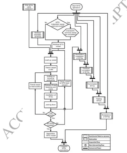
[image:10.595.66.478.199.693.2]WTG installation are shown in Figure 4, which
ACCEPTED MANUSCRIPT
11 provides a high-level view of the model structure for the installation of WTGs. Operations displayed
as sub-processes indicate that the operation is applied to all WTGs, and the sequencing shown in
Figure 4 applies to a single WTG. Onshore assembly of turbines is carried out prior to loading onto an
installation vessel, with the degree of assembly largely driven by the turbine manufacturers. The
degree of onshore assembly will dictate the number and complexity of offshore operations, and any
combinations of these onshore and offshore operations can be supported by the model. Once the
WTG is installed a number of supporting operations are required prior to the activation of the
turbine. Mechanical and electrical completion operations complete the installation, followed by
commissioning of the WTG. Once commissioned, final testing and acceptance are carried out, after
which the turbine can be activated and begin to generate power as required.
The general structure of the model for each asset installation is similar to that shown in Figure 4,
with the main differences arising in the modelling of the on-site offshore installation operations.
Figure 2 indicates the support operations which are required with the installation of the other key
assets. These include boulder clearance, pre-lay surveys and trenching of cable paths, post-lay cable
burial, mechanical and electrical completion operations on OSPs, grouting of foundations and the
commissioning of various assets.
Each operation modelled is described in terms of the operational limits and the required duration to
complete the operation. Factors such as contingency time required for each operation and random
vessel failures can also be considered. A large number of operational decisions can be defined, which
provide the flexibility to model many real-world installation scenarios. Pile-driven jacket foundations
can be installed through a pre- or post-piling approach, each support operation for the cable laying
can be included as required for a given set of site conditions, and various decisions dictate the use of
supply barges where appropriate. There are typically up to two OSPs on a given wind farm, and
these assets are substantially heavier than other assets installed above sea-level. As such, OSPS are
ACCEPTED MANUSCRIPT
12 equipped with suitable cranes for lifting. Due to these factors, the installation of OSPs can follow a
larger number of installation scenarios than is typical of other assets. For example, a single vessel
may fully install each OSP in turn, or may partially complete the installation of each OSP, before
returning to each OSP to complete the installation. Some of these decisions are investigated in
Barlow et al. (2014b).
3. Mixed-method offshore wind farm installation logistics framework
As the problem was being structured, different methodologies to model the installation project were
considered. Two models emerged as potential candidates for development; discrete event
simulation and optimisation, however both have different strengths and weaknesses with regard to
the scheduling of OWF installation logistics. A simulation model would be capable of providing a
realistic assessment of the duration of installation operations subject to uncertain weather
conditions; however, a large number of simulation runs (for example 1000 simulations) may be
required to ensure that robust estimates on the durations can be obtained. The computing time to
evaluate a single installation scenario could therefore be in the order of hours, and investigating
many installation scenarios could become infeasible.
Alternatively, an optimisation model could comfortably explore large decision-spaces to identify the
optimal scheduling of operations; however, each operation duration is defined as a specific value
within its range by a robust model. The result is that the assigned durations may not be
representative of their actual durations, so that schedules may be insensitive to seasonality, and the
benefits of operating during months with more favourable weather conditions cannot be exploited.
Instead of developing a single model or two models in isolation, a mixed-methods approach was
adopted where the complementary strengths of the simulation and optimisation models were
ACCEPTED MANUSCRIPT
13 optimisation mixed method approaches). A simulation model was developed in order to explore the
impact of starting operations at different months throughout the year. This would enable the
seasonality of the weather conditions to be fully considered in an installation schedule, and with a
relatively focused decision problem computing times would not be overly restrictive. An
optimisation model was developed to identify the optimal scheduling of operations from this
starting-point, with full exploration of the potential start-times for each set of operations possible; a
task that would be infeasible using the simulation model alone. The output of the optimisation
model would then be used by the simulation model to model the overall uncertainty and cost of the
installation project using a more detailed weather model. Both models were developed in Matlab,
and run off an Excel interface for user inputs. The remainder of this section describes the two
models.
3.1. Offshore wind farm installation logistics simulation model
The simulation model employs a synthetic weather time-series model to provide a realistic
estimation of how the installation operations will progress. A fuller description of the weather model
employed here is provided in Dinwoodie and McMillan (2014), in which the weather model is used
to analyse the effectiveness of maintenance operations for an OWF; however, the model is
summarised here for clarity. Synthetic weather time-series are generated from statistical analysis of
hindcast (historical) weather data sets. The method used here to generate synthetic weather
time-series is a correlated autoregression model. Autoregression identifies the underlying trends as a
data-set changes over time, and exploits these trends to predict future behaviour of the data-set. An
autoregression model expresses a given point as a linear combination of the previous
data-points. The general form of an autoregressive model of data-set at time-step is
ACCEPTED MANUSCRIPT
14 where is the mean of the data-set, is a random variation influencing the th data-point, is a
multiplicative factor acting on the th data-point before , and is the order of the model. The
extent of the dependency of a data-point on previous data-points is controlled by the model order
and the multiplicative factors ; these define how far back in time has an influence on the
current data-point and the extent of this influence. The existing hindcast data-set is analysed to
define the extent of the dependency on previous data-points such that the closest fit to the existing
data-set is produced. Future data-points are then generated iteratively using the same dependency
relationships.
The weather properties included here are significant wave height and wind speed. As discussed in
Dinwoodie and McMillan (2014), wind and wave time series require pre-processing such that the
mean and variance are stationary and the data approximates a normal distribution prior to the
application of autoregressive modelling. Equation (1) can then be applied to the transformed wind
and wave time-series to generate synthetic hourly weather series. Correlations between the wind
and wave data can be incorporated by correlating the random variations, , at each time-step
across both time-series.
The variability of the historical data-set influences the degree of uncertainty surrounding the
accuracy of predicted conditions. Consistently stable weather conditions can be predicted with a
relatively high level of certainty, whereas the accuracy for a prediction of highly transient weather
conditions is more uncertain. Each synthetic weather series generated through the autoregression
model is one prediction of future weather conditions at a particular location, and by taking many
predictions an accurate representation of the uncertainty associated with the predictions can be
obtained. The weather model is coupled with the logical installation model described in Section 2 in
the framework of a discrete-event simulation model. Discrete-event simulation is a widely used OR
technique for the analysis of complex systems. Recent examples of applications of discrete-event
ACCEPTED MANUSCRIPT
15 charging (Palensky et al. 2013, Darabi and Ferdowsi 2013), design and analysis of wood pellet supply
chains (Mobini et al. 2013), design and analysis of the supply chain for biocrude production (Eksioglu
et al. 2013), evaluation and management of smart grids (Al-Agtash 2013, Brown and Khan 2013),
scheduling and control of distribution circuits with photo-voltaic generators (Jung et al. 2015), and
operation and maintenance of OWFs (Endrerud and Liyanage 2014, Dinwoodie and McMillan 2014).
The discrete-event simulation model is a multi-threaded implementation, where each thread can
operate in parallel to other threads subject to specific logical constraints. The threads represent each
installation vessel, supply barge and support operation, and the constraints in each case are defined
by the logical installation model. Each thread maintains a clock which records the time transpired
since the global start of the installation project. The state of the model represents the current clock
for each thread, the current progress of the installation for each WTG, OSP, and cable, the location
of each vessel and barge (in-port or on-site), and the current number of assets carried by each vessel
and barge. Events are characterised as pre-installation support operations, in-port installation vessel
or barge operations, on-site installation vessel or barge operations, and post-installation support
operations, and each event results in some change to the state of the model. The first stage of the
simulation completes all pre-installation support operations for all assets, as these can be grouped
according to asset-type and each group is then completed independently. The main loop of the
simulation maintains a priority queue of the threads associated with installation vessels and barges,
where the level of priority is determined from the time of the thread clock and the satisfaction of
various constraints to ensure the logical structure of the installation model is adhered to.
Furthermore, priority is given to earlier operations in the sequence displayed in Figure 2 and
installation vessels are prioritised over supply barges, in order to reduce the computational burden
of processing constraint violations. The selection of each thread within the main simulation loop
triggers a sequence of events, with the particular sequence dependent on the selected vessel or
ACCEPTED MANUSCRIPT
16 of events characterised as on-site operations, a sequence of post-installation operations are
triggered, dependent on the type of asset in question.
For a given installation scenario, the simulation model estimates the progress of the installation
under each synthetic realisation of weather conditions through the discrete-event simulation model.
Metrics such as task durations, costs, progression and delays can be recorded for each simulation,
and the value recorded in each case will be dependent on the sensitivity of the metric to the
weather conditions and to the severity of weather conditions in the particular synthetic time series.
Repeating this process builds an uncertainty distribution for each metric, and by doing this across
many synthetic weather series an accurate representation of the expected impact of the uncertain
weather conditions is obtained. Figure 6 from the case study in Section 4 provides a typical example
of the uncertainty distributions for a particular metric; the metric in this case is the duration of use
for the WTG installation vessels, and each box-plot in Figure 6 shows the uncertainty distribution for
this metric for a particular start-date of operations.
The number of simulations used will therefore have a substantial impact on the accuracy of the
uncertainty distribution for each metric, and should be chosen to be sufficiently large so that an
acceptable level of accuracy is obtained. The process for ensuring the accuracy of the uncertainty
distribution for a given metric is discussed further in Barlow et al. (2014c). For example, for the case
study investigations presented in Section 4.1 the number of simulations is set to 1000.
In addition to historical weather data covering a suitable time-period, the simulation model requires
input data on the various vessels utilised during the installation. In particular, the capability of each
vessel to perform its designated tasks is required, including the operational weather and daylight
limitations for each task and the associated durations, which may be uncertain. Additional
information on the size and location of the site and all ports used is required. The nature of the
model enables a detailed breakdown of the simulated installation scenario to be produced, with
ACCEPTED MANUSCRIPT
17 site-level as well as per category of asset. Standard industry measures such as the 50th percentile and
the 90th percentile can be recorded for each output; however, these outputs are recorded for every
simulation so that a more complete understanding of the variation of each output is also provided.
This simulation model can therefore be utilised to explore the impact of a wide variety of logistical
decisions on the OWF installation. Considerations such as the number of vessels or barges used for
each type of asset installation, the operational capability of the vessels and barges, the impact of the
ports selected for use, and the scheduling of the various stages to the installation, can each be
explored in detail and validated. Section 4 demonstrates the application of this model to the
scheduling of multiple operations, and the model has been employed previously to explore the
impact on the installation duration and costs of: the operational characteristics of the installation
vessels (Barlow et al. 2014a), the use of the installation vessels and the selected installation strategy
(Barlow et al. 2014b), the size and composition of the installation vessel fleet (Barlow et al. 2014c),
and technological and operational advances to the installation process (Barlow et al. 2015).
3.2 Offshore wind farm installation logistics optimisation model
Developing a schedule for the installation operations of an OWF will identify crucial aspects of the
installation, including the expected progress of the installation, when critical operations are
expected to start, when vessels are required, and when the installation of each type of asset begins.
Key logistical installation decisions can then be supported, for example organising the delivery of
assets to ports, determining the vessel hiring dates and durations, and estimating the time interval
to hire crew for support installation operations. To correctly inform these decisions, the planned
baseline schedule should accurately represent the actual (observed) schedule. The installation of
large-scale OWFs is a long term process, during which many disruptions to the planned baseline
schedule can be expected. For example, the task durations may be longer or shorter depending on
ACCEPTED MANUSCRIPT
18 may become unavailable due to breakdowns, leading to delays in the tasks assigned to that vessel. A
realistic baseline schedule must therefore account for these unexpected disruptions.
There are many studies that incorporate uncertainty in creating baseline schedules based on
optimisation techniques; see Herroelen and Leus (2005) for a comprehensive survey. In this study,
we employ robust optimisation techniques to find the estimated task start times which minimise the
total project duration, subject to uncertain task durations. The resulting baseline schedule provides
an upper bound on the total project duration. To create this baseline schedule, we first determine
which tasks are assigned to each vessel, followed by the resulting durations and precedence
relations between the tasks. Our solution approach is thus composed of two stages: the first stage is
the initialization stage for the robust baseline schedule, in which we assign to each vessel the tasks
required to complete the installation; the second stage finds the robust baseline schedule solving an
optimisation model. The details of the first and second stages are explained in Sections 3.2.1 and
3.2.2, respectively.
3.2.1 Asset-vessel assignment algorithm
We develop an asset-vessel assignment algorithm to decide which tasks are performed by each
vessel, given the vessel and asset configuration of the OWF. The planner selects the vessels to be
used to install each type of asset, and the installation order of the assets in each case. The algorithm
then assigns assets to the appropriate vessels based on the asset installation order. With all assets
assigned, we structure the complete set of tasks to be performed by each vessel.
Consider, for example, an OWF with 100 turbines and two installation vessels with capacities of four
turbines each. The first asset to be installed is assigned to the vessel which can complete this
installation at the earliest time. We then update that vessel’s expected installation finish time to
account for all tasks required to install the first asset. The second asset to be installed is now
ACCEPTED MANUSCRIPT
19 fashion until all assets are assigned to vessels, we structure all tasks performed by each vessel, the
precedence relations between tasks, and the task durations. In this example, the first three tasks are
mobilisation, loading of four turbines, and transiting to site. The mobilisation task precedes the
loading task, consisting of four turbines being loaded, which precedes the transiting task.
The steps of the asset-vessel assignment algorithm are given below.
Step 1. Find assets that are not yet assigned to any vessel.
Step 2. Find the expected time to complete installation of the next asset for each vessel, considering
all tasks that have been assigned in each case.
Step 3. Assign the next asset to be installed to the vessel that has the shortest installation finish
time. If all assets are assigned to a vessel, terminate the algorithm. Otherwise go to Step 2.
The detailed calculations for the installation finish times are given in Tezcaner Öztürk et al. (2016).
3.2.2 Generating a robust schedule
The second stage of our approach generates the baseline schedule for all tasks of the installation by
utilizing robust optimisation methods. In their seminal paper, Bertsimas and Sim (2004) developed a
robust model allowing a subset of constants, which are subject to uncertainty, change their values
within an interval defined by minimum and maximum values. In a project scheduling context,
Minoux (2009) solves program evaluation and review technique (PERT) scheduling problem with a
two-stage robust linear programming model based on the approach developed by Bertsimas and Sim
(2004). They consider only precedence relations between tasks as constraints. Our method is also
based on Bertsimas and Sim (2004) approach, but we consider a more general case. For the OWF
installation problem, we schedule a large number of tasks subject to three constraint sets:
precedence relations, task ready times, and task deadlines. A precedence relation constraint is
ACCEPTED MANUSCRIPT
20 task of a turbine that can start only if the asset is transported to the site, the installation vessel is
present at the installation site and is idle, and the inter-array cable(s) for that turbine is (are)
installed. These make three predecessor tasks for the installation task of this turbine. We should
note that, in the meantime, installation of other turbines can be ongoing, and their installations do
not affect the installation of other turbines. If some vessels begin operating after the start date of
the project, or some operations cannot start before a specific date, we set ready times for the tasks
of these vessels and operations. The ready times are conceptually different than the precedence
relations between tasks, such that they determine the start time of the first task of a vessel. The
ready times are user-defined parameters and they depend on the contracts for the vessels and ports
rather than the progress of the installation operations.
A developer may commit to begin generation before the whole installation finishes, which is
commonly agreed as a percentage of generating capacity available from an export generation date.
We refer to these export generation dates as task deadlines. The model decides on the start times of
the tasks to minimise the total duration of the installation project, subject to all constraints.
The mathematical programming model we develop has two levels. The inner level aims to find an
overall schedule that minimises the total project duration with deterministic task durations. The
outer level determines the sensitivity of the project duration to variations in durations of different
tasks, and thus identifies which task variations have the greatest impact on the project duration. We
combine both levels in a single mathematical programming model and solve them simultaneously.
Let denote the set of tasks, be the set of tasks with deadlines, and be the set of
tasks with ready times. We introduce two dummy tasks to the task set: initial task 0 and the final
task . Let the set include all tasks pairs for which task precedes task
denote the deadline of task denote the ready time of task and denote the
duration of task We include all tasks without an immediate predecessor to and if they do
ACCEPTED MANUSCRIPT
21 to for tasks that do not have any successor task. We assume [ ] where
is the nominal value (under no deviation) and , with defining the
range of duration values for task . The model decides on the start times of each task and
minimises , i.e., the start time of the final task. is a parameter representing the maximum
number of tasks whose duration can deviate within their interval, and denotes the extent to
which the duration of task deviates.
Maximise Minimise
∑ , (2)
(3)
(4)
(5)
The inner model finds an optimal schedule for a set of tasks by setting the task start times, the
decision variables for , that minimise the total duration of the project. The task durations are
taken as Constraint (2) ensures that if task precedes task task cannot
start before task is completed. If task has a deadline, constraint (3) ensures that task should be
completed before its deadline. Similarly, if task has a ready time, constraint (4) ensures that task
cannot start before its ready time. Since task 0 is the initial task and all other tasks are preceded by
it, setting the start time of this task greater than zero is enough in constraint (5). The outer model
finds the maximum total duration of the project if task durations are assumed to take values
within their interval. The outer model decides on the values of to obtain the highest
possible increment in the total duration of the project. We remark that intermediate task
completions are not necessarily estimated for their individual worst case scenarios in such a
schedule, as only the total project duration is evaluated for its worst case, however, such completion
ACCEPTED MANUSCRIPT
22 optimisation model by dualising the inner model. Since the ’s are parameters to the inner model
but decision variables for the overall model, we have the multiplication of two decision variables in
the objective function of the combined model; the variables and the dual variables corresponding
to constraints (2) and (3). We linearize the resulting nonlinear model using additional binary
variables. The details of these steps can be seen in (Tezcaner Öztürk et al., 2016). The final linear
model has as many binary variables as the number of immediate precedences between tasks, and
this does not increase the computational burden of the model; installation projects with thousands
of tasks can be solved in a few minutes.
The overall problem finds a robust schedule for deviating tasks satisfying constraints (1)-(4), and an
OWF planner can decide on the percentage of tasks that may vary from their nominal values. can
be obtained by multiplying the percentage of deviating tasks with the total number of tasks, and
can take any positive value. If the model reduces to a deterministic LP: there is no need to
solve the robust model as in the outer model, and it is sufficient to solve the inner
model by setting the duration of each task to If more than two schedules have the same
project duration, we select the schedule with the least cost, as detailed in Tezcaner Öztürk et al.
(2016). We make a remark regarding the range of task durations: The minimum value can be seen as
the shortest duration with perfect weather conditions and crew capability, while the maximum value
being the longest duration when the weather conditions do not permit the task to start immediately.
Finally, we also make a technical remark that, unlike the models presented in Bertsimas and Sim
(2004) and Minoux (2009), our model does not necessarily generate extreme case solutions with all
variables but one set to either 0 or 1, as it incorporates deadlines.
The model generates a robust schedule for a percentage of tasks deviating from their nominal
durations, while satisfying the precedence, ready time, and deadline constraints. Solving only the
inner model to obtain a schedule by setting the durations of the tasks to their expected values could
ACCEPTED MANUSCRIPT
23 advantage of this robust schedule is that the project duration proposed by the model is guaranteed
to be greater than or equal to the actual duration of a project with a given percentage of deviating
tasks. Moreover, if the tasks with deviation are different to those proposed by the model, the
schedule still remains feasible. Optimal project durations will be naturally increasing while the value
of increases.
The input for the optimisation model is taken through an Excel Interface, and the optimisation
model is prepared to be solved by one of the following optimisation software packages: CPLEX, FICO
Xpress, or MATLAB. The results of the model (the Gantt chart for the operations of the vessels, the
total project duration and cost) are then reported in the same Excel sheet. Given that there are five
distinct high-level vessel operations, followed by five support operations at each WTG, in addition to
various vessel operations (such as transiting between port and site), the total number of tasks are
around a few thousands for large OWFs. Presenting the Gantt chart for an OWF with hundreds of
assets would not be practical and would provide little clarification to the reader, however, we
present an example Gantt chart in Figure 5 for the installation of 10 turbines using two installation
vessels. Some tasks are
Figure 5: An example Gantt chart for operations of two vessels for the installation of 10 turbines
grouped to provide a better understanding of the schedule. The vessels have different performances
and thus their task durations vary, but both finalize their tasks by day 27.
1 2 3 4 5 6 7 8 9 10 11 12 13 14 15 16 17 18 19 20 21 22 23 24 25 26 27 WTG Installation Vessel 1
Mobilisation Preparation
Installation of WTG group 1 Transit back
Demobilisation WTG Installation Vessel 2 Mobilisation
Preparation
Installation of WTG group 2 Transit back
Demobilisation
ACCEPTED MANUSCRIPT
24 We also developed a rolling horizon algorithm to optimise the scheduling of the remaining tasks to
finalise installation. This algorithm can be used throughout the installation process, when the OWF
planner sees substantial deviations from the baseline schedule, and there is a need to find new
estimates for project completion time, activation dates for vessels, etc., or when new vessel options
arise. The algorithm uses the two steps (asset-vessel assignment algorithm and generating a robust
schedule) as we use in creating the baseline schedule, this time separating the planning horizon into
two: fixed period and planning period. Fixed period spans the duration of the tasks that are already
assigned to the vessels, and we allocate the remaining tasks to the vessels during their planning
periods. The details of this algorithm can be seen in Tezcaner Öztürk et al. (2016). In creating a
robust baseline schedule, our aim is to provide a worst-case bound on the project duration; and the
respective project cost and estimates for vessel/operation activation dates. The companies require
estimates on these such that the arrangements for the installation project should be done before
the installation starts. For example, some of the vessels need to be reserved in advance with high
costs of lease as there is a competitive demand from various industries such as oil and gas, and
hence changing such decisions often can be very costly. Although it is possible that the progress of
the project is not going in line with the initial plan, the rolling horizon algorithm is capable of
generating new schedules at different points in time, and to suggest updated bounds on the project
duration, and updated vessel/operation activation dates.
4. Case study: supporting decision making throughout an offshore wind farm installation
To demonstrate the capability of the simulation and optimisation model discussed in Section 3, a
case study of an offshore wind farm installation is investigated. This case study was developed in
collaboration with industry partners and is designed to give a general representation of the next
phase of OWF installations in Europe. The input parameter values were provided by the industry
partners based on their combined experience from previous OWF installation projects; however,
ACCEPTED MANUSCRIPT
25 The site studied here is shown in Figure 6 and consists of 120 WTGs with 6 MW generating capacity
and 2 OSPs connected through 127 inter-array cables. Each OSP has two parallel export cables, each
consisting of four offshore sections and a single nearshore section. The site is located in the North
Sea 80 Nautical Miles (NM) off the East coast of the UK with an average water depth of 50 m.
To populate the weather model discussed in Section 3, high-quality time-series weather data is
required. For the purposes of this study weather data from the FINO1 weather research station is
used, which is located in the North Sea 50 km off the coast of Germany (Bundesministerium fuer
Umwelt 2012). While the conditions recorded at FINO1 may differ from a particular site off the coast
of the UK, this data enables the capability of the simulation and optimisation models to be
demonstrated with realistic weather data.
Sections 4.1 and 4.2, respectively, present the application of the simulation and optimisation
components of the holistic scheduling approach presented in Section 3 to the case study OWF. For
the sake of brevity the analysis is restricted to the installation of the 120 WTGs of the case study.
Two identical high-performance WTG installation vessels are utilised, which are capable of installing
turbines up to wind speeds of 10 m/s and transiting at 12 knots with a full load up to significant
ACCEPTED MANUSCRIPT
26 Figure 6: Layout of the case study offshore wind farm site
heights of 2 m. The installation operations are shown in Figure 4, with support operations consisting
of mechanical and electrical completion, commissioning, testing and acceptance.
4.1 Scheduling installation operations with consideration of seasonality
For the investigations below, 1,000 simulations are performed for each start-date considered, with
1,000 simulations found to provide an acceptable level of statistical accuracy; further information on
this process can be found in Barlow et al. (2014c).
For the sake of brevity, the starting date for the WTG installation is considered here in terms of the
impact on the duration of vessel operations. The cost per day for the WTG installation vessels can be
expected to be substantially more expensive than costs for the installation technicians required to
complete the WTG support operations. Minimising the duration of the WTG vessel operations is
therefore a reasonable approach; however, in practice a more sophisticated investigation could be
performed, as is discussed in Section 4.3. Figure 7 shows the variation in the combined duration of
both installation vessels, as the vessel mobilisation dates are varied from an original date of 1st May
over the course of one year. All preceding operations are assumed to be completed at times such
that these will not delay the installation vessel operations. It is evident from Figure 7 that
ACCEPTED MANUSCRIPT
27 Figure 7: The impact on the combined duration of both WTG installation vessels, as the vessel
start-date is varied over the course of one year
selection of the start-date for installation vessel operations has a substantial impact on the resulting
operation durations. A start-date in March produces the shortest vessel durations on average, with a
combined total for both installation vessels of approximately 440 days. In contrast, a start-date in
August produces the longest vessel durations on average, at approximately 570 days for both vessels
combined. A single WTG installation vessel therefore operates for between approximately 7.5-9.5
months of the year. The duration is minimised by fully exploiting the summer months and more
favourable weather conditions, and by minimising the exposure to the winter months and delays
resulting from harsher weather conditions.
4.2 Scheduling installation operations with optimal staggering of operations
The case study is now solved using the robust optimisation model to obtain an understanding of how
the tasks progress overall and to suggest activation dates for the support operations to the WTG
installation. The base-case activation date for the installation vessels is 243 days after the start-date
ACCEPTED MANUSCRIPT
28 assets are to be installed, the optimisation model suggests activation dates for each vessel, which
would be useful for planning vessel-hire contracts.
We apply the optimisation model for different percentages of deviating tasks, with findings shown in
Table 1, where durations are adjusted relative to the start-date of the installation vessels. We recall
that the robustness parameter is obtained by multiplying the percentage of deviating tasks with
the total number of tasks. The last five columns of Table 1 show the estimated activation dates for
each support installation operation under the worst case scenario for total project duration. The
results are obtained using CPLEX solver.
Table 1: Project Duration, Project Cost, and Activation Dates for Different Percentage of Deviating
Tasks Percentage of Deviating Tasks Total Project Duration (days) Total Project Cost (k£)
Activation Dates (Days After Start Date of Installation Vessels) Mechanical Completion Electrical Completion Commiss-
ioning Testing
Accept-ance
5% 555.28 111,665.34 156.04 156.68 157.32 234.96 235.28
10% 731.50 140,829.44 332.26 332.90 333.54 411.18 411.50
25% 949.54 182,152.81 539.87 540.51 543.98 605.33 605.65
50% 949.54 184,575.30 535.24 538.70 539.35 614.13 615.41
The total project duration is determined by the series of consecutive tasks that form the longest
path, which is referred to as the critical path. The optimisation model sets the duration of the tasks
on the critical path to their upper bounds and finds the longest possible project duration. For
different percentages of deviating tasks, the resulting project duration will be the same if the
number of tasks on the critical path is less than the number of deviating tasks. As more task
durations are allowed to deviate from their nominal values, both project duration and project cost
increase as expected; however, the resulting schedules become more robust to changes in the task
durations, which is particularly crucial when weather conditions are volatile.
Before we discuss results regarding varying percentages of deviating tasks, we make a technical
ACCEPTED MANUSCRIPT
29 sum of percentage deviations of all individual tasks. For example, if we set 10% of tasks to deviate
for a system with 20 tasks (hence setting ) a feasible solution can have any combination of
deviations for individual tasks (the variables ) as long as their sum is bounded by 2. This could
therefore be achieved by 2 tasks deviating to their maximum possible duration while the remaining
18 tasks take their minimum duration values with no deviation (hence ∑ 1+1≤2), or by each of
the 20 tasks having a deviation of 0.1 to their maximum possible duration (hence ∑ 20x0.1≤2).
We note that when we search the critical path in a robust network setting, the optimal solutions
naturally tend to the extreme cases where deviations are equal to either one or zero, as indicated
with the first solution to the numerical example above for the case of 20 tasks and . Although
this observation is noted for models such as those presented in Bertsimas and Sim (2004) and
Minoux (2009), we remark that our model does not necessarily generate such extreme case
solutions, as it incorporates deadlines.
If 5% of the tasks are assumed to deviate from their nominal durations, the estimated time to start
support operations is approximately 156 days after the installation start-date. This estimation might
be valid for an installation project that spans mostly spring-summer months; where the tasks do not
deviate much due to weather conditions. As the percentage of deviating tasks increases to 50%, the
suggested activation dates increase to approximately 535 days after the installation start-date. This
estimation, on the contrary, refers to a project that spans mostly winter months, and the task
durations show considerable variability. The increase in the activation dates results from the
increase to the critical paths from longer vessel operation durations. We also remark that this
represents a relatively extreme case, resulting in half of the tasks hitting their longest expected
durations. The activation dates of electrical completion and commissioning are marginally delayed
from the mechanical completion start-date; however, there is a gap between the activation dates of
commissioning and testing operations for all percentages of deviating tasks. Acting in conservative
fashion, the optimisation model finds the latest start for all the support operations, guaranteeing
ACCEPTED MANUSCRIPT
30 duration of testing is much shorter than the commissioning operation, leading to this gap between
their activation times.
Determining the percentage of deviating tasks usually requires expert judgement to decide on the
weather conditions for the total installation duration. The installation generally spans a few years
(the installation of 120 turbines takes 2-3 years as given in Table 1), and it is generally not
straightforward to determine the variability of task durations. OWF developers need to test different
values based on their expert judgements and evaluate the schedules generated. If the installation
is mostly carried out during summer months, a lower percentage of deviating tasks will be more
representative of the installation. If the installation spans primarily winter months, the percentage
of deviating tasks might be set to a larger value.
4.3 Discussion
Sections 4.1 and 4.2 illustrated the mixed-method scheduling approach presented in Section 3. This
approach is one method of hybridising these models; however, there are various alternatives which
could be explored. As indicated in Section 4.1, an alternative application is to give a more
sophisticated consideration of the impact of varying the start-date. The optimisation model could be
applied as a preliminary step to identify the optimal scheduling of the different sets of operations, as
demonstrated in Section 4.2. This would provide a schedule which is optimal with respect to the
average yearly weather conditions. The simulation model could then be used to explore this
schedule of operations, and to investigate perturbations to the yearly average optimal schedule as
the start-date is varied throughout the year. This would provide an optimal schedule for each month
of the year. However, the approach presented in Section 4.1 was thought to provide a more concise
and straightforward demonstration of these models.
An alternative hybridisation would be to use the simulation model to identify the tasks which are
ACCEPTED MANUSCRIPT
31 nominal value. This information could be used to explicitly define the deviating tasks in the
optimisation analysis, rather than using the deviation percentage defined through and automating
the selection of the deviating tasks. This additional information would provide an analysis which is
more representative of the progress that would actually be observed in a real installation
application.
The above investigations focus on the duration of operations, however, in reality this is only one
factor for an OWF developer, and the date from which power can be generated and exported to the
onshore grid would also be taken into consideration. Each of these factors has an economic impact
on the viability of the OWF, and a balance between low installation costs (through low durations of
vessel use) and early generation (through completing operations as quickly as possible) must be
achieved.
5. Verification, Validation and Application
The models were developed to be used to inform installation strategies for upcoming OWFs by the
industry partners involved in their development. Upon completion, the models were subjected to
verification and validation by those within the project team and external experts. Due to the limited
number of OWFs that have been installed and the lack of reliable data to benchmark the model
output to, industry partners agreed that a pragmatic approach to validation was required. Phillips
(1984) defines a requisite model as one such that “its form and content are sufficient to solve the
problem”. Three different activities were carried out to verify and validate the model.
First, the model code was subjected to external verification from a mathematical software
consultancy to review and interrogate the implementation of the logistical model and the logical
structure of the code. They confirmed that the code was an accurate representation of the logical
structure agreed by the industry collaborators. Second, the model was benchmarked against an
ACCEPTED MANUSCRIPT
32 identified, these were discussed with industry experts. In particular, the weather model employed
here provides improved accuracy in uncertainty quantification for durations and costs. Furthermore,
the framework developed here enables flexible and reactive assignment of tasks when multiple
vessels install the same asset, which is more representative of task assignment in practice. Finally,
engineers within the two industry organisations explored multiple case studies to ensure that the
model was fit for purpose. This included ensuring that the output was adequate to support the
decisions necessary and that the output could be interrogated sufficiently to identify the cost and
uncertainty drivers within the installation process. Based on these verification and validation steps,
the models have now been adopted by industry partners to inform installation strategy
development.
This framework is currently being used by SSE Renewables (one of our collaborating industry
partners) to support decision making for the logistical planning of the Beatrice OWF installation
project, a 600 MW wind farm located off the North-East coast of the UK which is scheduled for
installation over 2017-2019. The framework has been fundamental to the decision-making process
since the earliest stages of installation planning, and has enabled each stage of the installation to be
interrogated. The capability to perform a detailed analysis, comparison and optimisation of
alternative options to a variety of decisions has enabled in-depth exploration of these decisions, and
the iterative development of the installation plan as decisions are fine-tuned, pursued or
abandoned.
SSE Renewables estimate that the use of this framework has delivered a saving of approximately
14% (tens of millions of GBP) of the installation costs, compared with initial cost estimates. These
savings have been brought about by improving the efficiency of the installation operations, primarily
with respect to the installation of the turbine foundations, the inter-array cables and the OSPs. The
framework presented here facilitated improvements by providing a mechanism to quantitatively
ACCEPTED MANUSCRIPT
33 indicative example of this is applying the tools to investigate the efficiency of the available jacket
installation techniques and how these can be deployed across the site. For each scenario considered,
the most efficient scheduling approach for the jacket installation vessels and all follow-on operations
is identified and compared, enabling informed decisions to be made. The same process is then
applied to explore the available options for the pile installation, and for each subsequent installation
operation.
6. Conclusions
The next phase of offshore wind farms (OWFs) to be developed in Europe in the coming years will
typically consist of hundreds of turbines, and will be located further from shore in deeper water than
has previously been encountered (Renewable UK 2014). The installation of these sites will typically
span several years and cost upwards of £100 million (Kaiser and Synder, 2010). Limited industry
experience on projects of these scales and location characteristics motivates the need for
decision-making support for developers, to ensure that operations are planned as efficiently as possible and
that the vast installation costs are streamlined where possible.
This paper describes the integration of a pair of complementary decision support models for the
installation of an OWF. Both models can be applied at the planning and bidding stages of an
installation, with each model supporting specific aspects of installation scheduling. An OWF
installation case study is investigated to demonstrate the potential capability of this integrated
framework to provide decision support to an OWF developer planning an installation campaign. The
scope is restricted here to the installation of the wind turbines for brevity; however, a similar
approach to that outlined here could be applied to the installation of all OWF assets. The framework
presented here could be adapted to model a variety of processes where operations are subject to
uncertain weather conditions, including tasks during the operation and maintenance or
decommissioning (removal of an asset from active status, including deconstruction of the structure)
ACCEPTED MANUSCRIPT
34 Future developments of this mixed methods framework will explore more efficient interfacing
between the simulation and optimisation components. Section 4.3 highlights an approach which
would make explicit use of the simulation model to define the required robustness of the
optimisation solution. This approach could be utilised even further by restructuring the optimisation
model to handle specific ranges of task durations which are defined by the simulation model for a
particular operation in a given timeframe. To utilise the simulation model in this way may require
development of a meta-model for the simulation model, such that the many duration outputs can be
generated in a tractable timescale within the optimisation run. The resulting model would implicitly
combine the detailed weather sensitivity of the simulation model with the superior scheduling
ability of the optimisation model, thus provide a powerful decision-support tool for OWF developers.
Acknowledgements
This study was funded through the University of Strathclyde Technology and Innovation Centre,
grant reference TIC/LCPE/FI03. The authors thank industrial partners Scottish Power Renewables,
SSE Renewables and Technip Offshore Wind Limited for their contribution to this work. Additionally,
the authors thank the Bundesministerium fuer Umwelt (Federal Ministry for the Environment,
Nature Conservation and Nuclear Safety) and the Projekttraeger Juelich (project executing
organisation) for climate data from the FINO project.
References
Ait-Alla A, Quandt M, Lutjen M (2013) Aggregate Installation Planning of Offshore Wind Farms. In:
Proceedings of the 7th international conference on communications and information technology
(pp. 130-135). Cambridge, MA, USA.