Modeling of single mode optical fiber having a complicated refractive index profile by using modified scalar finite element method

City, University of London Institutional Repository

Citation

: Raghuwanshi, S.K. & Rahman, B. M. (2016). Modeling of single mode optical

This is the accepted version of the paper.

This version of the publication may differ from the final published

version.

Permanent repository link:

Link to published version

: http://dx.doi.org/10.1007/s11082-016-0632-9

Copyright and reuse:

City Research Online aims to make research

outputs of City, University of London available to a wider audience.

Copyright and Moral Rights remain with the author(s) and/or copyright

holders. URLs from City Research Online may be freely distributed and

linked to.

City Research Online: http://openaccess.city.ac.uk/ [email protected]

1

Modeling of Single Mode Optical Fiber having a Complicated Refractive

Index Profile by using Modified Scalar Finite Element Method

1_{Sanjeev Kumar Raghuwanshi and} 2_{B. M. Azizur Rahman} .

1,2_{Instrumentation and Sensor Division, School of Engineering and Mathematical Sciences,} Northampton Square, City University London, EC1 V 0HB, UK

1_{Corresponding Author: [email protected]}

Abstract

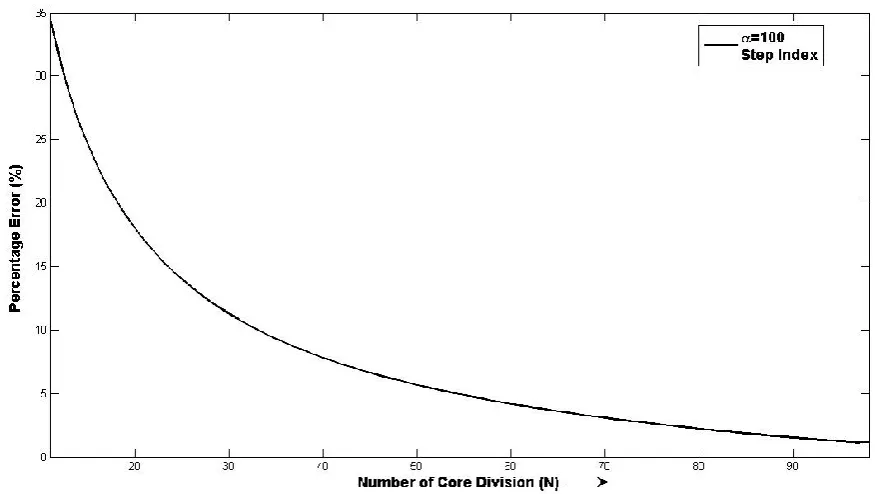
A numerical method based on modified scalar finite element method (SC-FEM) is presented and programmed on MATLAB platform for optical fiber modeling purpose. We have estimated the dispersion graph, mode cut off condition, and group delay and waveguide dispersion for highly complicated chirped type refractive index profile fiber. The convergence study of our FEM formulation is carried out with respect to the number of division in core. It has been found that the numerical error becomes less than 2 % when the number of divisions in the core is more then 30. To predict the accurate waveguide dispersion characteristics, we need to compute expression numerically by the FEM method. For that the normalized propagation constant (in terms of ) should be an accurate enough up to around 6 decimal points. To achieve this target, we have used 1 million sampling points in our FEM simulations. Further to validate our results we have derived the higher order polynomial expression for each case. Comparison with other methods in calculation of normalized propagation constant is found to be satisfactory. In traditional FEM analysis a spurious solution is generated because the functional does not satisfy the boundary conditions in the original waveguide problem, However in our analysis a new term that compensate the missing boundary condition has been added in the functional to eliminate the spurious solutions. Our study will be useful for the analysis of optical fiber having varying refractive index profile. Keywords: Chirp Type’s refractive index profile, waveguide dispersion, group delay, finite element method (FEM)

1.

Introduction

2

The optical fibers can be in various structural dissimilarities just like in photonic crystal fiber has various size or shapes of holes. Many critical steps may involve during these type of optical fibers fabrication process [1-5]. The modeling process plays an important role in the development of optical fibers and related devices by evaluating the geometrical design performance such as guiding properties, mode confinement capability to mention few. Optical waveguide modeling techniques can be divided into analytical and numerical methods. Numerical methods are preferred whenever the analytical solution is not possible for certain geometry like in photonic crystal optical fiber. For the numerical methods, several approaches, this includes the scalar or vectorial finite difference method, scalar or vectorial finite element method, and Beam propagation method are preferred. Apart of that a semi-analytical method has also developed to analyze a taper optical waveguide [6-12]. Instead of finite element method, finite difference method may also be preferred in certain cases due to easier formulation procedure; however accumulation of truncation error and long computation time may reduce the method feasibility. In order to overcome these problems in this paper we opted the finite element method analyses in order to produce acceptable simulation results while shorten the time. In case of weakly guiding approximation, we can efficiently use the scalar wave equation solution instead of fully vectorial method for complicated waveguides. Indeed in this paper we use the weakly guiding approximation throughout for all the cases like chirped/alpha power refractive index profile. It then obtained the scalar wave equation by ignoring the terms for the interaction between two polarized field components in the vectorial wave equations. Since in our FEM formulation we are dealing with a single mode fiber with degenerate mode (HE11 mode having same polarization state in

principal), hence the error generated by scalar FEM while compared to vectorial FEM is negligible [13-31].

2.

Finite element method analysis of optical fibers

In this section, variational formulation based on FEM analysis of the HE11 mode in optical fibres

having a complex refractive-index profile is described. Figure 1 reveals the core region where the refractive index can be an arbitrary profile. The maximum refractive index of the core is denoted as and that in the cladding as . The wave equation correspond to HE11 mode is given, by with as [12-14]

(

) ( )

3

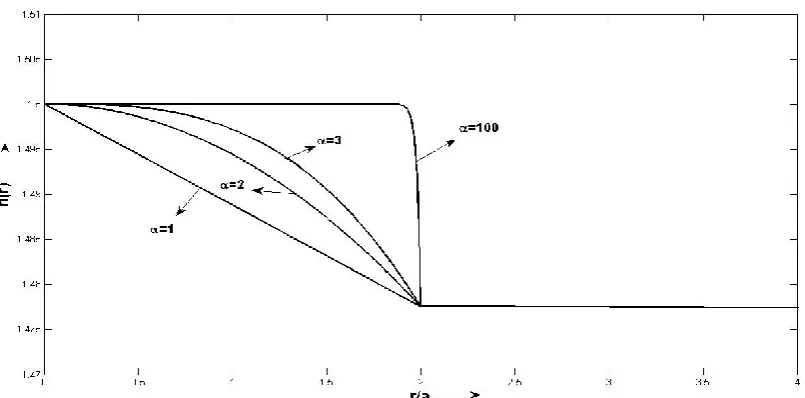
Fig. 1: Refractive-index distribution and schematic of - power refractive index distribution of inhomogeneous optical fiber, where ‘a’ is the core radius.

Before transforming eq. (1) into a variation expression, the waveguide parameters are normalized as

where and corresponds to the core and cladding interface. Following this normalization, the wave equation and the boundary condition are rewritten as

(

) [ ]

_}

Here the transverse wavenumber , the normalized frequency and the normalised refractive index profile are given by

√

√

}

The solution of the wave eq. (3) under the constraint of the boundary condition can be obtained as the solution of the variational problem that makes the functional stationary: as follows [15-25]

[ ] ∫ (

) ∫ [ ]

4

{

∑

where are the field values at the sampling points to be solved and is 0th order modified Bessel function. Also

( )

}

The solutions in the cladding and the substrate are given by the analytical functions. The sampling function becomes unity at , becomes zero at the neighboring sampling points and , and is zero throughout all other regions. The precise expressions of are given by,

{ ( )

{

( ) ( )

( ) ( )

{ ( ) ( )

Since the sampling function here is a linear function of , eq. (6) means that the continuous function

is approximated by the broken lines. The normalized refractive index distribution is also approximated, by using the sampling function, as

∑

( )

Substituting eq. (6) in eq (5), we obtain the functional

∫ (

) ∫ [ ]

5

3.

Modeling of Graded Types Refractive Index Profile of Single mode Optical fiber

Once the eigenvalue equation for matrix as described in “Appendix A.2 is solved to find the allowed values of wave propagation constant leading to obtain the corresponding eigenvector

by simple matrix operation. Here is obtained with respect to

, while is still yet to find out. The total optical power has to be normalized to obtain . Figure 1, show the -power refractive index profiles given by [23, 25], for an optical fiber and planar slab waveguide respectively

{ ( )

{

| |

}

The planar slab waveguide is a basic structure through one can design various types of integrated

optical waveguide structure. In this paper the objective is to compare the circular core fiber case with

planar slab waveguide case. This is because the coordinates are different but the wave equation is

same for both the cases [32-34]. Hence the validity of the results can be established better. Next, we

shows the results of FEM analyses for HE11 of optical fiber while comparing with TE modes of planar

6

Fig. 2: Cutoff normalized frequency of optical fiber for HE11 mode with -power refractive-index profiles.

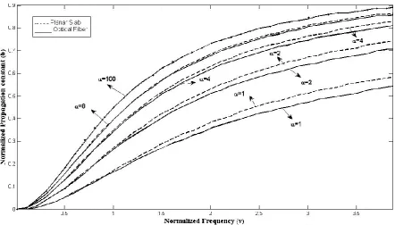
From the observation of the Figure 4 , it is apparent that the planar slab waveguide behaves more or less similarly as an optical fiber near cut off frequency (low -number range of for any type of profile. However the triangular profile shows much difference in their behvior far from cut off region. We can also conclude that the fundamental mode of an optical fiber HE11 behaves in a similar

way as TE01 mode of planar slab waveguide for step index profile case.

7

Fig. 4: Normalized propagation constant of optical fiber (HE11 mode) and planar slab (TE01 mode) waveguides with -power refractive-index profiles.

Figure 4 also reveals that in case of triangular profile case the power of fundamental mode is more tightly confined in the core region of optical fiber hence these properties can be used for strongly guided fiber applications. Cross sectional view of the electric field and magnetic field vectors for the case of is shown in Fig. 5. It is apparent from this plot that vector is perpendicular to

field vector. The plot of component for the case of mode is shown in Fig. 6. Figures 5 and 6

corresponds to and ( and ) at while computed allowed value of . Once the propagation constant is known for

entire wavelength of interest to us we can predict the dispersion characteristics of an optical fiber or a waveguide having a complex refractive index profile. After knowing the normalized propagation

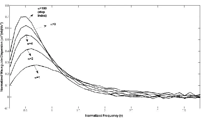
characteristics we can calculate and for any type of refractive index profile case. Further we can calculate the waveguide dispersion by using the following expression [23-25],

8

Fig. 5: Cross sectional view of the a) electric field and b) magnetic field vectors for the case of

mode.

9

Fig. 7: Normalized delay

of optical fiber with -power refractive index profiles.

Fig. 8: Normalized waveguide dispersion parameter

of optical fiber with -power refractive index

profiles.

10

is discussed in next section. To compute the waveguide dispersion the value of normalized propagation constant should be an accurate enough up to at least 6 decimal points.

4.

Modeling of Linearly Chirp Types Refractive Index Profile of Single mode Optical

fiber

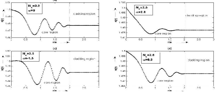
In this section we will apply our finite element formulation further to estimate the waveguide dispersion for chirped refractive index profile. Now here we define a variety of more complicated than previous case a generalized linear chirp type refractive index profile and is defined as [31-32],

{

{ | | } ( | |) { }

where is the refractive index at the center of the waveguide at , controls the growth or decay of the profile envelope, is the number of cycles in a core radius, is the core radius and is the cladding refractive index. The refractive index profile can be divided into two parameters. One, the fiber parameters like , and other, the profile parameters like and . By varying these parameters , we can generate profiles from simple step index type to complex multiple cladding type as shown in Fig. 9. For an example the profile parameters are and

respectively for step index profile. Figures 10-12 shows the normalized propagation constant ,

propagation constant in terms of and normalized group delay for the mode of optical

fiber having linear chirp types of refractive-index profiles. The waveguide dispersion can be computed straight forward from the Fig. 12 and eq. (15).

11

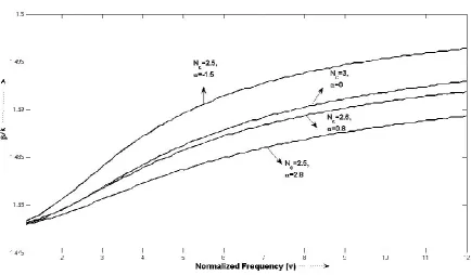
Fig. 10: Normalized propagation constant of optical fiber with linear chirp types of refractive-index profiles.

Fig. 11: Propagation constant in terms of as a function of for optical fiber with linear chirp types of refractive index profiles.

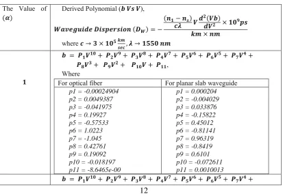
12

more accurate results we have derived the higher order polynomial equations, which established the relationship mathematically between and -number. Using the described polynomial equations, we can get the similar result and more accurate response of the waveguide dispersion. The polynomial equations, which describe the relation between and -number represented in Fig. 4 can be shown by the Table 1.

Fig. 12: Normalized delay

of optical fiber with linear chirp types of refractive index profile.

Table 1: The Polynomial equation derived for the Fig. 4 The Value of

Derived Polynomial ( ),

where

,

Where

For optical fiber For planar slab waveguide

p1 = -0.00024904 p2 = 0.0049387 p3 = -0.041975 p4 = 0.19927 p5 = -0.57533 p6 = 1.0223 p7 = -1.045 p8 = 0.42761 p9 = 0.19092 p10 = -0.018197 p11 = -8.6465e-00

p1 = 0.000204 p2 = -0.004029 p3 = 0.033876 p4 = -0.15822 p5 = 0.45012 p6 = -0.81141 p7 = 0.96319 p8 = -0.8419 p9 = 0.6101 p10 = -0.072611 p11 = 0.0010013

13

,

Where

For optical fiber For planar slab waveguide

p1 = -0.00037675 p2 = 0.007179 p3 = -0.058293 p4 = 0.26239 p5 = -0.70978 p6 = 1.1518 p7 = -0.98619 p8 = 0.11705 p9 = 0.50663 p10 = -0.028838 p11 = -0.00082955

p1 = 0.00024924 p2 = -0.0052164 p3 = 0.046329 p4 = -0.22793 p5 = 0.6825 p6 = -1.3001 p7 = 1.6465 p8 = -1.514 p9 = 1.0357 p10 = -0.096414 p11 = 0.00048899

,

For optical fiber For planar slab waveguide

p1 = -0.00031762 p2 = 0.0065332 p3 = -0.057385 p4 = 0.28011 p5 = -0.82426 p6 = 1.4626 p7 = -1.399 p8 = 0.32131 p9 = 0.54558 p10 = 0.0070741 p11 = -0.00037985

p1 = -3.6107e-005 p2 = 0.0010183 p3 = -0.011741 p4 = 0.071828 p5 = -0.25014 p6 = 0.47631 p7 = -0.34605 p8 = -0.35521 p9 = 0.78986 p10 = -0.028264 p11 = 0.0004006

,

where

For optical fiber For planar slab waveguide

p1 = 0.000305 p2 = -0.0060284 p3 = 0.050768 p4 = -0.23862 p5 = 0.69406 p6 = -1.3341 p7 = 1.8337 p8 = -1.9496 p9 = 1.4209 p10 = -0.078954 p11 = 0.00066221

p1 = -0.00021593 p2 = 0.0043746 p3 = -0.037495 p4 = 0.17534 p5 = -0.47508 p6 = 0.69546 p7 = -0.28413 p8 = -0.70926 p9 = 1.0689 p10 = -0.042595 p11 = 0.00017185

,

Where

For optical fiber For planar slab waveguide

p1 = -0.00058377 p2 = 0.011559 p3 = -0.096856 p4 = 0.44456 p5 = -1.1997 p6 = 1.8512

14

On the basis of the polynomial mentioned in table 1, we can obtain the same result represented in the Fig. 4, Fig. 7 and Fig. 8 as shown in the Fig. 13.

Fig. 13 Simulation result obtained by the derived polynomial represented in the Table 1: (a) -number relation (b)

- number relation (c)

-number relation (d) Waveguide dispersion for

different value of .

Figure 13 shows that, we are able to obtain the similar results using the derived polynomials represented in the table 1. Fig. 13(a) shows the versus -number relation similar to the Fig. 4. On

the basis of this, we can calculate the response for represented in the Fig. 13(b) and 13(c), respectively. Finally, we can calculate the waveguide dispersion, represented in the Fig. 13(d). Hence, this shows that we can consider the derived polynomial as an appropriate mathematical equation for the calculation of the waveguide dispersion. In the same manner, we can show the higher

p7 = -1.2765 p8 = -0.41813 p9 = 1.1734 p10 = -0.041564 p11 = -0.00018982

15

order polynomial equations, which show the similar result equivalent to the Fig. 10 and Fig. 12. The table 2 shows the derived polynomial equation.

Table 2: The Polynomial equation derived for the Fig. 11 Derived Polynomial ( )

where ,

Where, the constant in above relation for various parameter values are

p1 = 1.3805e-009 p2 = -8.7842e-008 p3 = 2.3409e-006 p4 = -3.3688e-005 p5 = 0.00028054 p6 = -0.0013427 p7 = 0.0035993 p8 = -0.0078156 p9 = 0.029432 p10 = -0.0091198 p11 = 0.0001478

p1 = 2.1628e-010 p2 = -1.2027e-008 p3 = 2.2808e-007 p4 = -7.5238e-007 p5 = -3.4104e-005 p6 = 0.00054423 p7 = -0.0032432 p8 = 0.0046619 p9 = 0.02717 p10 = -0.0096538 p11 = 0.00013959

p1 = 8.3385e-010 p2 = -4.6045e-008 p3 = 9.5012e-007

p4 = -7.3996e-006 p5 = -2.8064e-005 p6 = 0.00095846 p7 = -0.0069776 p8 = 0.01881 p9 = 0.0050421 p10 = 0.00062066 p11 = -0.00065062

p1 = -1.5755e-009 p2 = 1.2441e-007 p3 = -4.2415e-006 p4 = 8.141e-005 p5 = -0.00095935 p6 = 0.0070577 p7 = -0.031 p8 = 0.068473 p9 = -0.028334 p10 = 0.013013 p11 = -0.0014513

Fig. 14 Simulation result obtained by the derived polynomial represented in the Table 2: (a) -number relation (b) -number relation (c) -number (d) Waveguide dispersion for

16

On the basis of the derived polynomial equations the waveguide dispersion plot can be represented as shown in the Fig. 14 (d). It is apparent while comparing Fig. 13(d) with Fig. 14(d) that in case of complicated chirped type profile case, the waveguide dispersion is flat and negative. Earlier also the profile as shown in Fig. 9 (c), has been analyzed in greater detail for the case of circular core fiber [26]. In literature [26], it has been shown; ⁄ waveguide dispersion over the band, but in our case the waveguide dispersion is even smaller as well as flat over the band as reveal in Fig. 14(d). From the Fig. 14(d), it is also apparent that the optimum parameter for lower waveguide dispersion is , corresponds to Fig. 9 (c).

5.

Conclusion

In the conclusion of the paper, we have characterized the dispersion property of linearly chirp

types of refractive index profile. The accuracy of FEM has been tested with respect to the

number of core division. We have achieved very good agreement with the previously

published results. It has been demonstrated that the numerical error becomes less than

for the number of the core divisions in FEM analyses

. Our study also reveals that the

optimum chirped type of refractive index profile waveguide can be used to achieve the flat

waveguide dispersion property over the band. This study will be useful in optical

communication systems where low dispersion link has to be deployed.

Commercial software

which obeys only the certain geometrical guide-lines, instead our method is flexible to

analyze for all type of geometrical shape of holes in the core for photonic crystal fiber.

Moreover the accuracy of our FEM method found to be up to 6 decimal points which are

sufficient enough to compute the waveguide dispersion and performance is well

comparable to commercial software.

Acknowledgment

This work is prepared as part of the post doctorate research work done by Dr. Sanjeev Kumar

Raghuwanshi under the project of Erasmus Mundus Scholarship program in a collaboration

between City University London, United Kingdom and Indian School of Mines Dhanbad,

Jharkhand India. This project has been funded with support from the European Commission.

This publication reflects the views only of the author, and the Commission cannot be held

responsible for any use which may be made of the information contained therein.

17

Appendix I

A.1 Derivation of eq. (13)

Since from eq. (5)

∫ (

) ∫[ ] We can split the above integration as follow,

∫ (

) ∫[ ] ∫ (

)

∫[ ]

As we know that

{

∑

Observing the equation (A.1) and (A.2), we can write, since hence

∫ (

) ∫[ ] ∫ (

)

∫[ ]

Taking the last two term of eq. (A.4) and putting the values of R using equation (A.3), we can write

∫ [

( )] ∫ ( ) Since,

, hence we can modify the expression (A.4) as follow

[∫ ∫ ] Now Since,

∫ { }

{

[ ]

[ ]

From Eq. (A.5),

18

∫ [ ]

In the same manner,

∫ ∫ ( )

∫ [ ]

Now putting the values of the expression from eq. (A.8) and (A.9) in eq. (A.5), we get

[ [ ] [ ]]

Finally, we can write the above expression,

[ ]

Since we know the identity,

[ ]

From eq. (A.11) and (A.10), we can write, [ ]

Putting the value, from eq. (A.12) in the eq. (A.10), we can write

Hence, we can write,

∫ [ (

)] ∫ ( )

Finally, it turns out to be

∫ (

) ∫[ ]

A.2 Derivation of eigenvalue equation using stationary condition

19

∫

∫ ∫

Substituting eq. (11) and eq. (12) in Eq. (A.16) and calculating the stationary conditions in

the same way as those in re [12]

_{order simultaneous equations are obtained. In}

order that Eigen value equations have nontrivial solutions except for

the determinant of the matrix

should

where the matrix elements of C are given by

(

)

[

]

[

]

[

]

}

where discretization step

is given by

. When the refractive index distribution

of the fiber and the normalized frequency

are given, the propagation constant

(implicitly

contained in

) is calculated from eq. (A.17) and eq. (A. 18).

References

[1].

Zheludev., Nikolay, I.: Photonic-plasmonic devices: a 7-nm light pen makes its

mark. Nat. Nanotechnol. 5, 10-11 (2010)

[2].

Politano, A., Chiarello, G.: Quenching of plasmons modes in air-exposed

grapheme-Ru contacts for plasmonic devices. Appl. Phy. Lett. 102, 201608

(2013)

[3].

He, X. Y., Wang, Q. J., Yu, S. F.: Numerical study of gain-assisted terahertz hybrid

plasmonic waveguide. Plasmonics. 7, 571-577 (2012)

[4].

Baqir, M. A., Choudhary., P. K.: Dispersion characteristics of optical fibers under

20

[5].

Li, Z.; Bao, K., Fang, Y., Huang, Y., Nordlander, P., Xu, H.: Correlation between

incident and emission polarization in nanowire surface plasmons waveguide.

Nano. Lett. 10, 1831-1835 (2010)

[6].

Politano. A., Chiarello, G.: Unravelling suitable grapheme-metal contacts for

grapheme-based plasmonic device. Nanoscale. 5, 8251-8220 (2013)

[7].

Mussina, R., Selviah, D. R., Fernnandez, F. A., Tijhuis, A. G., Hon, B. P. D.: A rapid

accurate technique to calculate the group delay dispersion and dispersion slop

of arbitrary radial refractive index profile weakly-guiding optical fibers.

Progress in Electromagnetic Research. 145, 99-113 (2014)

[8].

Walpita, L. M.: Solution for planar optical waveguide equation by selecting zero

elements in a characteristics matrix. Journal of the Optical Society of America.

A2, 592 – 602 (1985)

[9].

Rahman, B. M. A.: Finite element analysis of optical waveguides. Progress in

Electromagnetic Research. 10, 187 – 216 (1995)

[10]. Raghuwanshi, S. K., Kumar, A.: A new semi-analytical method for the analysis of

tapered optical waveguide. Optik (Elsevier). 125(24), 7515 – 7221 (2014)

[11].

Honkis, T. H.: Analysis of optical waveguide with arbitrary index profile using an

immersed interface method. International Journal of Modern Physics C. 22(7),

687 – 710 (2011)

[12].

Okoshi, T., Okamoto, K.: Analysis of wave propagation in inhomogeneous optical

fibers using a varational method. IEEE Trans. On Microwave Theory and Tech.

MTT-22(11), 938 – 945 (1974)

[13].

Popescu, V. A.: Determination of normalized propagation constant for optical

waveguide by using second order variational method. Journal of Optoelectronics

and Advanced Mat. 7(5), 2783 – 2786 (2005)

[14].

Rostami, A., Motavali, H.: Asymptotic iteration method: a power approach for

analysis of inhomogeneous dielectric slab waveguide. Progress in

Electromagnetic Research B. 4, 171-182 (2008)

[15].

Chaudhuri, P. R., Roy, S.: Analysis of arbitrary index profile planar optical

21

[16].

Sadiku, M. N. O.: Numerical techniques in electromagnetic: Second Edition CRC

Press LLC (1992)

[17].

Booton, R. C.: Computational methods for electromagnetic and microwave. John

Wiley and Sons. (1992)

[18].

Kasim, N. M., Mohammad, A. B., Ibrahim, M. H.: Optical waveguide modeling

based on scalar finite difference scheme. Journal Teknologi. 45(D), 181-194

(2006)

[19].

Gambling, W. A., Payne, D. N., Matsumura, H.: Cut-off frequency in radically

inhomogeneous single mode fiber. Electron. Letters. 13(5), 130 – 140 (1977)

[20].

Zhuangqi, C., Jiang, Y., Yingli, C.: Analytical investigation of planar optical

waveguide with arbitrary index profiles. Optical and Quant. Electronics. 31, 637

– 644 (1999)

[21].

Chiang, K. S.: Review of numerical and approximation methods for modal

analysis of general dielectric waveguide. Opt. Quantum Electron. 26, 113 – 134

(1994)

[22].

Xu, W., Wang, Z. H., Huang, Z. M.: Propagation constant of a planar dielectric

waveguide with arbitrary refractive index variation. Opt. Lett. 18, 805 – 807

(1993)

[23].

Okamoto, K.: Fundamentals of optical waveguide. Academic Press (2006)

[24].

Sharma, E. K., Goyal, I. C., Ghatak, A. K.: Calculation of cut-off frequencies in

optical fibers for arbitrary profiles using the matrix method. IEEE Journal of

Quant. Electron. QE-17(12), 2317 – 2320 (1981)

[25].

Okamoto, K., Okoshi, T.: Analysis of wave propagation in optical fibers having

core with

-power refractive distribution and uniform cladding. IEEE Trans. On

Microwave Theory and Tech. MTT-24(7), 416 – 421 (1976)

[26].

Raghuwanshi, S. K., Kumar, S.: Analytical expression for dispersion properties of

circular core dielectric waveguide without computing

numerically.

I-manager’s Journal on Future engineering & Technology. 7(3), 26-34 (2012)

[27].

Ghatak, A. K., Thyagarajan, K.: Optical electronics: introduction to fiber optics.

Cambridge Press (1999)

[28].

Hotate, K. A., Okoshi, T.: Formula giving single-mode limit of optical fiber having

22

[29].

Rostami, A., Moyaedi, S. K.: Exact solution for the TM mode in inhomogeneous

slab waveguides. Laser Physics. 14(12), 1492 – 1498 (2004)

[30].

Survaiya, S. P., Shevagaonkar, R. K.: Dispersion characteristics of an optical fiber

having linear chirp refractive index profile. IEEE Journal of Lightwave Tech.

17(10), 1797 – 1805 (1999)

[31].

Raghuwanshi, S. K., Talabattula, S.: Dispersion and peak reflectivity analysis in a

non-uniform FBG based sensors due to arbitrary refractive index profile.

Progress in Electromagnetic Research B. 36, 249-265 (2012).

[32].

S. K. Raghuwanshi, and B. M. A. Rahman “Analysis of Novel Chirped Types of

Refractive Index Profile Metamaterial Planar Slab Optical Waveguide by Finite

Element Method for Sensor Application”

IEEE Sensor Journal,

vol. 15, no. 7.pp.

4141-4147, 2015

[33].

Sanjeev Kumar Raghuwanshi, and B. M. Azizur Rahman, “Propagation and

Characterization of Novel Graded and Linearly Chirped Type’s of Refractive Index

Profile Symmetric Planar Slab waveguide by Numerical Means”,

Progress in

Electromagnetic Research-B

(MIT-USA), vol. 62, pp. 255-275, 2015.

[34].

Sanjeev Kumar Raghuwanshi, Santosh Kumar,Ajay Kumar “Dispersion

characteristics of complex refractive-index planar slab optical waveguide by using