General optimized lower and upper bounds for discrete and continuous arithmetic Asian options

City, University of London Institutional Repository

Citation

:

This is the accepted version of the paper.

This version of the publication may differ from the final published

version.

Permanent repository link:

Link to published version

:

Copyright and reuse:

City Research Online aims to make research

outputs of City, University of London available to a wider audience.

Copyright and Moral Rights remain with the author(s) and/or copyright

holders. URLs from City Research Online may be freely distributed and

linked to.

Discrete and Continuous Arithmetic Asian Options

Gianluca Fusai

Dipartimento SEI, Universit`a del Piemonte Orientale & Cass Business School, City University London,[email protected] & [email protected]

Ioannis Kyriakou

Cass Business School, City University London,[email protected]

We propose an accurate method for pricing arithmetic Asian options on the discrete or continuous average in a general model setting by means of a lower bound approximation. In particular, we derive analytical expressions for the lower bound in the Fourier domain. This is then recovered by a single univariate inversion and sharpened using an optimization technique. In addition, we derive an upper bound to the error from the lower bound price approximation. Our proposed method can be applied to computing the prices and price sensitivities of Asian options with fixed or floating strike price, discrete or continuous averaging, under a wide range of stochastic dynamic models, including exponential L´evy models, stochastic volatility models, and the constant elasticity of variance diffusion. Our extensive numerical experiments highlight the notable performance and robustness of our optimized lower bound for different test cases.

Key words: arithmetic Asian options; CEV diffusion; stochastic volatility models; L´evy processes; discrete average; continuous average

MSC2000 subject classification: Primary: 91B70, 91B25, 60J25; Secondary: 60H30, 91B24

OR/MS subject classification: Primary: asset pricing, diffusion, Markov processes, stochastic model applications

1. Introduction. We develop accurate analytical pricing formulae for discretely and con-tinuously monitored arithmetic Asian options under general stochastic asset models, including exponential L´evy models, stochastic volatility models, and the constant elasticity of variance dif-fusion. The payoff of the arithmetic Asian option depends on the arithmetic average price of the underlying asset monitored over a pre-specified period. For more than two decades, much effort has been put into the research on efficient methodologies for computing the price of this option or, in general, expected values of functionals of the average value, under different model assumptions for the underlying. Developing such methods is of considerable practical importance as arithmetic aver-ages see wide application in many fields of finance. Amongst others, we mention uses in computing net present value in project valuation (see [72]), optimal capacity planning under average demand uncertainty for a single firm (see [32]) and stock-swap merger proposals (see [60]). Weighted arith-metic averages also appear in technical analysis and in algorithmic trading; for example, we recall the moving average trading rule and its use from an asset allocation perspective (see [75]). Moving average automatic trading strategies set buying and selling orders depending on the position of the average price for a given period with respect to the current market price (see [50]). Finally, weighted arithmetic average indexes are used as trading benchmarks in pension plans (see [11]).

Arithmetic Asian options are very popular among derivatives traders and risk managers. Their appeal stems mainly from the fact that averaging smooths possible market manipulations occurring near the expiry date. Moreover, averaging provides suitable volatility reduction and better cash-flow matching to firms facing streams of cash cash-flows. Due to these nice features, Asian options

are particularly appropriate for currency, energy, metal, agricultural and freight markets and, unsurprisingly, represent a large fraction of the options traded in these markets.

To be able to reproduce stylized properties of the asset prices in the various markets, it is nec-essary in many cases to depart from the basic lognormal model by incorporating, for example, random jumps, stochastic volatility and mean-reversion in the price dynamics. Unluckily, the pric-ing of arithmetic Asian options does not admit true analytical solutions, even under the lognormal model, as the distribution law of the arithmetic average is not known analytically. In fact, the advantage of a more realistic model specification is often offset by the need to implement compu-tationally expensive numerical procedures, where available. It is, thus, the main objective of this paper to present a simple, accurate and fast pricing formula, albeit approximate, for arithmetic Asian options allowing flexible modelling of the underlying asset price dynamics, filling this way an important long-standing gap in the literature.

A large volume of publications is devoted to the pricing of Asian options, mainly, with continuous monitoring in the Black–Scholes economy. Without being exhaustive, we mention Rogers and Shi [61], who are the first to provide the Asian option price by solving a partial differential equation (PDE) in one space dimension, but also Veˇceˇr [69] and Zhang [74] with improved PDE-based solutions in low-volatility settings; Linetsky [53] derives an elegant spectral expansion for the option price; Geman and Yor [42] are the first to give a solution in terms of a single-Laplace transform, which is re-derived in Dewynne and Shaw [31] where it is shown how to treat the low-volatility case more effectively. An also accurate double-transform at low volatility levels is suggested in Fusai [38], whereas Cai and Kou [14] generalize to a double-Laplace transform under the hyperexponential jump diffusion model, encompassing the Gaussian model and Kou’s double exponential jump diffusion as special cases. Veˇceˇr and Xu [70] show that the option price satisfies a partial integro-differential equation (PIDE) in the case of exponential L´evy price dynamics, which is solved numerically in Bayraktar and Xing [9] for the special case of jump diffusion models. Finally, Ewald et al. [36] propose a solution under the Heston model by means of a PDE and a Monte Carlo simulation method, whereas Yamazaki [71] a pricing formula based on the Gram-Charlier expansion. Another stream in the literature is concerned with pricing discretely monitored Asian options. We mention, amongst others, contributed works by Andreasen [3] and Veˇceˇr [69] based on PDE approaches under lognormal asset price dynamics and the Fourier transform-based recursive convolution of Carverhill and Clewlow [20] on a reduced state space, whereas enhanced variations of the latter under general exponential L´evy dynamics appear, for example, in Benhamou [10], Fusai and Meucci [40], ˇCern´y and Kyriakou [21] and Zhang and Oosterlee [73]. Beyond the L´evy framework, Dassios and Nagaradjasarma [29] and Fusai et al. [39] obtain explicit prices for Asian options under the square root asset price dynamics ([55] consider a modified version with independent jumps added), whereas Cai et al. [15] and Sesana et al. [64] develop, respectively, an efficient asymptotic expansion and a quadrature method applicable to the generalized constant elasticity of variance (CEV) diffusion.

the cases of non-random deterministic or independent stochastic interest rates. Finally, Lemmens et al. [52] apply the conditional expectation technique to obtain lower bounds for the prices of discrete arithmetic Asian options in the general exponential L´evy asset price model.

Although earlier methods relying on L´evy log-increments of the underlying are found to be impressively fast and accurate (e.g., see [40], [21] and [73]), lack of such an assumption, as, for example, in the case of stochastic volatility models or the CEV diffusion, poses nontrivial mathe-matical and computational challenges. Our lower bound price approximation aims to tackle these difficulties efficiently. Following Curran [28], Rogers and Shi [61], Thompson [67] and Lemmens et al. [52], we devise suitable conditioning variables under different stochastic dynamic models and monitoring frequencies (discrete or continuous). In general, our method relies on identifying suitable averages of the underlying asset prices, for use as conditioning variables, which have analytically tractable laws and are close proxies to the original arithmetic average so that a tight lower bound is eventually obtained. More precisely, for exponential L´evy and stochastic volatility models we use the (log) geometric mean, whereas for the CEV diffusion we resort to the generalized (power) mean. Using only knowledge of the underlying asset price law (jointly with the stochastic volatility where assumed) via the associated characteristic function, we provide a general explicit recursive algorithm which gives us access to the bivariate characteristic function of the asset price and the new average. Given this, and beyond the original contributions of Curran [28] and Rogers and Shi [61], we derive an analytical solution for the lower bound in the Fourier domain, similarly to Lemmens et al. [52] under exponential L´evy models. This is then recovered by a single univariate inversion and sharpened using simple optimization.

Our proposed method is distinguished from other pricing methodologies for Asian options due to a number of appealing features. First, it can be applied flexibly to a wide range of non-Gaussian models, such as pure jump L´evy models, Merton’s normal and Cai and Kou’s generalized hyperex-ponential jump diffusions, models with/out jumps in the asset price/volatility dynamics, and the CEV diffusion, without restricting to models admitting time changed Brownian (L´evy) representa-tions which may not be always common or straightforward to use. Second, we provide interesting theoretical findings related to the pricing of Asian options in the CEV diffusion model, which requires special treatment due to its distinct distributional properties. Third, in the absence of symmetry relations between fixed and floating strike Asian options beyond the exponential L´evy asset price model (see [34]), by a slight modification of the conditioning variables and a change of num´eraire, we are able to switch from fixed to floating strike option price results. Fourth, with slight modification of the pricing formulae, we can obtain the option price sensitivities with respect to parameters of interest. Moreover, for first time in the literature, we provide a formulation which applies also to continuous Asian options under general model assumptions. The final line of research that we contribute to in this paper is concerned with deriving a theoretical upper bound to the error made in our optimized lower bound price approximation that can be calculated numerically. To verify the efficiency of the proposed methodology, extensive numerical experiments are con-ducted to compare the accuracy of our optimized lower bound with existing methods in the lit-erature against benchmarks generated by a very accurate control variate Monte Carlo simulation strategy which uses as control variate the lower bound itself. To make concrete our analysis, we investigate the numerical performance of our lower bound in a wide range of L´evy models, volatil-ity models and the CEV diffusion, for options with varying moneyness and monitoring frequency (monthly, weekly, daily, continuously). In summary, our numerical experiments demonstrate the high accuracy of our optimized lower bound, with notable performance even for extremely low volatilities, and its robustness in all the aforementioned test cases. The method is also fast and simple to implement requiring a single univariate transform inversion, while the problem dimension remains unaffected by the additional random volatility factor.

Section 3 presents our transform representations of the lower bounds to the Asian option prices under different contract specifications (fixed strike or floating strike price), monitoring frequencies and model specifications. For the same cases, we present in Section 4 expressions for the error in our lower bound price approximation. Section 5 is devoted to our numerical study. Section 6

concludes.

2. Market models and preliminary results. Assume that the price of the underlying asset S is observed at the equally spaced discrete times t0≡0, t1≡∆, . . . , tj≡∆j, . . . , tN ≡∆N =T,

where T is a fixed time horizon. We assume a filtered probability space (Ω,_F,F_{≡(Ft)t∈[0,T],}P₎

where P_{is the risk neutral probability measure.}

2.1. L´evy models. Assume that X_≡lnS is represented by a L´evy process, i.e., satisfies the general form

dXt=εdt+σdWt+dLxt,

where ε_∈R _{is deterministic, σ≥0 constant, W a standard Brownian motion and L}x _{a purely}

discontinuous random process. Consider the log-increments of the underlying

lnS∆j−lnS∆(j−1)=X∆j−X∆(j−1)≡Zj∆, (1)

so that the price of the underlying asset at tj is

S∆j=S0eZ

∆ 1+···+Zj∆

forj= 1, . . . , N. At the level of risk neutral modelling, exponential L´evy asset price models allow to generate implied volatility smiles and skews similar to the ones observed in market prices. Under such model assumptions, the increments (1) are independent and identically distributed. By the celebrated L´evy–Khintchine formula, the characteristic function ofZ∆

j has the form

E_[exp(iuZ∆

j )]≡exp(ψ∆(u))≡exp(iuε∆ +ϕ∆(u)) (2)

for allj, whereϕ∆(u) =ψ∆(u)−iuε∆. Further, we choose

ε=r₋q₋ 1

∆ϕ∆(−i) =r−q−ϕ1(−i), (3)

where r_≥0 and q_≥0 denote respectively the constant instantaneous risk-free interest rate and dividend yield, to ensure that the discounted asset price is a martingale under the probability measureP_{, e.g., see Schoutens [62], which is necessary for the risk neutral pricing of derivatives.}

For our purposes, it is also necessary to specify the asset price dynamics under the measure P

where the underlying itself represents the num´eraire, see Geman et al. [41]. From the num´eraire change formula, the characteristic function of Z∆

j under the measureP has the form

E_[exp(iuZ∆

j )] =E[exp(−r∆ +i(u−i)Zj∆)] = exp(−r∆ +ψ∆(u−i)). (4)

2.2. Affine stochastic volatility (ASV) models. When the risk neutral dynamics of the log-priceXis given by a L´evy process, the implied volatility surface follows a deterministic evolution (see [23]). Stochastic volatility models can tackle this difficulty. More specifically, diffusion-based volatility models account for dependence in increments and long-term smiles and skews, but cannot give rise to realistic short-term implied volatility patterns. This shortcoming can be overcome by introducing jumps in the returns and in the evolution of the volatility. To this end, a number of ASV models have been introduced in the literature. Popular examples include the time changed L´evy processes proposed by [18] and [19], where the time change is given by integrated Ornstein– Uhlenbeck (OU) or square root variance processes, with special cases being these of the Heston and Barndorff–Nielsen–Shephard (BNS) models based on time changed arithmetic Brownian motions (e.g., see [49]), the Bates and Duffie–Pan–Singleton (DPS) models, the Stein–Stein and Sch¨obel– Zhu model with mean-reverting Gaussian volatility dynamics, which is affine with the state vector augmented by the squared volatility (e.g., see [48]), but also members from the affine GARCH class (see [56]). While our proposed method (see Section3) can be readily applied to pricing Asian options under the aforementioned model assumptions requiring only knowledge of the characteristic function of the driving affine process, for ease of exposition we focus here attention on the Heston, Bates, DPS and BNS cases.

Under the risk neutral measure, the Heston model [46] is described by the following stochastic differential equations

dXt= (r−q−Vt/2)dt+

p

Vt(ρdWt+

p

1₋ρ2_dB t),

dVt=α(β−Vt)dt+γ

p

VtdWt,

where B, W are independent standard Brownian motions, α, β, γ are positive constants and ρ_∈ [₋1,1] is the instantaneous correlation coefficient between the log-asset price process X and the variance processV. The Bates model [8] is an extension of the Heston model to include jumps in the (log) asset price dynamics

dXt= (r−q−lk(1)−Vt/2)dt+

p

Vt(ρdWt+

p

1₋ρ2_dB

t) +dLxt,

where Lx _{is a time-homogeneous compound Poisson process with intensity l >0 and normal}

dis-tribution of jump sizes ξx with mean µx∈R and standard deviation σx≥0 and k(u)≡exp(µxu+

σ2

xu2/2)−1. The DPS model introduced in Duffie et al. [33], in addition to the jumps in the

(log) asset price process, includes contemporaneous jumps in the variance process. The governing equations are

dXt= (r−q−lk(1,0)−Vt/2)dt+

p

Vt(ρdWt+

p

1₋ρ2_dB

t) +dLxt,

dVt =α(β−Vt)dt+γ

p

VtdWt+dLvt,

whereLv _andLx_{are driven by a common Poisson process, hence jumps occur concurrently in both}

processes, however the jump sizes ξv have exponential distribution with mean µv>0. Also, the

magnitudes of the jumpsξx andξv have a correlation determined by the parameterρx,v; given ξv,

the jump sizes ξx are normally distributed with mean (µx+ρx,vξv) and variance σ2x. Under this

model specification,k(u1, u2)≡exp(µxu1+σ2xu12/2)/(1−ρx,vµvu1−µvu2)−1.

L´evy-driven positive OU processes are also of particular interest in the context of stochastic volatility modelling. Barndorff-Nielsen and Shephard [6] and Barndorff-Nielsen et al. [5] suggest the so-called BNS model of the form

dXt= (r−q−lk(ρ)−Vt/2)dt+

p

VtdWt+ρdLt,

where parametersρ_≤0,l >0,W is a standard Brownian motion andL is the background driving L´evy process, which is a subordinator without drift and is independent of W. We consider two popular parametric specifications of the BNS model, namely the BNS-Γ and BNS-IG model, where the OU process (5) respectively has a gamma (Γ) stationary distribution with k(u)_≡νu/(α₋u) for some ν, α >0, and an inverse Gaussian (IG) stationary distribution withk(u)_≡νu/√α2_−2u

for someν, α >0.

Affinity of the volatility models described above implies that the characteristic function of the pair (V, X) has exponentially affine dependence onV andX, i.e., there existϕ∆, ψ∆:iR2→Csuch

that

E_{[exp{iuV∆(j+1)+iυX∆(j+1)}|F∆j] = exp{ϕ∆(iu, iυ) +ψ∆(iu, iυ)V∆j+iυX∆j},}

or, equivalently, from (1)

E_{[exp{iuV∆(j+1)+iυZ}∆

j+1}|F∆j] = exp{ϕ∆(iu, iυ) +ψ∆(iu, iυ)V∆j}. (6)

Using the num´eraire change formula, we also obtain under the measureP

E_{[exp{iuV∆(j+1)+iυZ}∆

j+1}|F∆j] = exp{−r∆ +ϕ∆(iu, i(υ−i)) +ψ∆(iu, i(υ−i))V∆j}. (7)

In Table 1, we provide the functionsϕ, ψ for the Heston, Bates, DPS and BNS models.

2.3. CEV diffusion model. Among the one-dimensional Markov processes, the CEV diffu-sion of Cox [24] is an important asset price model which has interesting analytical properties and can flexibly provide good fits to various shapes of implied volatility curves observed in the market-place by varying the elasticity parameter γ. Despite its economic importance, the CEV diffusion has been studied less in the literature of Asian options pricing. In this model, the underlying asset price dynamics under the risk neutral measure is given by

dSt= (r−q)Stdt+σSγ/2t dWt, σ≥0, γ∈R.

Cox [24] originally studied the caseγ <2, whereas Emanuel and MacBeth [35] extended his analysis to the case γ >2 (see also [63]). The special case of γ= 1 corresponds to the well known square root process of Cox and Ross [25], whereas when γ= 2 we obtain the lognormal model. The CEV diffusion with γ = 1 has been applied to the pricing of arithmetic Asian options in Dassios and Nagaradjasarma [29], Fusai et al. [39] and, more recently, in its general form in Cai et al. [15], Sesana et al. [64] and Cai et al. [16].

A useful property of this model for the purposes of our application in Section3is the following: forX_≡S2−γ_{, we get from Itˆo’s lemma}

dXt = (r−q)(γ−2)

σ2_(γ

−1) 2(r₋q) −Xt

dt+σ(2₋γ)pXtdWt. (8)

Model (8) is affine in the state variable and can be characterized by its moment generating function (see [51, Proposition 6.2.4]),

E_[e−µX∆(j+1)_|F

∆j] = exp{ϕ∆(0, µ)−ψ∆(0, µ)X∆j}, (9)

where

ϕ∆(ν, µ) ≡

γ₋1 γ₋2ln

2θe((r−q)(γ−2)−θ)∆/2

(σ2_(2−γ)2_{µ+ (r−q)(γ−2))(1−e}−θ∆_{) +θ(1 +e}−θ∆₎

, (10)

ψ∆(ν, µ) ≡

(θ(1 +e−θ∆_{)−(r−q)(γ−2)(1−e}−θ∆_{))µ+ 2(1−e}−θ∆_)ν

(σ2_(2−γ)2_{µ+ (r−q)(γ−2))(1−e}−θ∆_{) +θ(1 +e}−θ∆₎ (11)

andθ_≡θ(ν)_{≡ |}γ₋2_|p

2.4. Discrete average. In light of the lack of analytical tractability of the law of the dis-crete arithmetic average of the asset prices 1

N+1

PN

j=0S∆j, we look for close proxies with known

distributional properties. More specifically, such a proxy is given by

Y∆N≡

1 N+ 1

XN

j=0X∆j, (12)

whereX= lnS in the case of the L´evy and ASV models of Sections2.1and2.2, whereasX=S2−γ

in the case of the CEV diffusion of Section 2.3. Important to our arithmetic Asian option pricing framework of Section3is knowledge of the distribution law of the new average (12). In Propositions

1,2and3, we derive key results under the L´evy, ASV and CEV diffusion models for use in Section

3.

Proposition 1. Define

ηj(u, υ) =

    

   

υ1_−Nj₊₁, k_∨n < j_≤N u+υ1₋ j

N+1

, k_∧n < j_≤k_∨n

2u+υ1_−Nj₊₁, 0< j_≤k_∧n

(13)

and

φk,n,N(u, υ) =E[exp{iu(X∆k+X∆n) +iυY∆N}]

under the risk neutral measure.

(i) (L´evy models). Under the assumption of increments Z∆

j satisfying (2), define

Ψh,∆(u, υ) =

XN

j=h+1ψ∆(ηj(u, υ)),

whereh= 0, k_∧n, k_∨n. Then,

φk,n,N(u, υ) = exp{i(2u+υ)X0+ Ψ0,∆(u, υ)}. (14)

(ii) (ASV models).Under the assumption of increments Z∆

j satisfying (6), define

Ψh,∆(u, υ;V∆h) =

XN

j=h+1ϕ∆(ϑj(u, υ), iηj(u, υ)) +ψ∆(ϑh+1(u, υ), iηh+1(u, υ))V∆h,

whereh= 0, k_∧n, k_∨nand ϑj satisfies the recursive equation

ϑj≡ψ∆(ϑj+1, iηj+1) (15)

for j=N₋1, . . . ,1 with ϑN ≡0. Then,

φk,n,N(u, υ) = exp{i(2u+υ)X0+ Ψ0,∆(u, υ;V0)}. (16)

Proof. See Appendix A.

Proposition 2. Define

¯

ηj(u, υ) =

 



−2u₋υ_Nj₊₁, k_∨n < j_≤N −u₋υ_Nj₊₁, k_∧n < j_≤k_∨n −υ_Nj₊₁, 0< j_≤k_∧n

(17)

and

¯

φk,n,N(u, υ) =E[exp{iu(X∆k+X∆n−2X∆N) +iυ(Y∆N−X∆N)}]

(i) (L´evy models). Under the assumption of increments Z∆

j satisfying (4), define

¯

Ψh,∆(u, υ) = exp

−r∆(N₋h) +XN

j=h+1ψ∆(¯ηj(u, υ)−i)

,

whereh= 0, k_∧n, k_∨n. Then,

¯

φk,n,N(u, υ) = ¯Ψ0,∆(u, υ). (18)

(ii) (ASV models).Under the assumption of increments Z∆

j satisfying (7), define

¯

Ψh,∆(u, υ;V∆h) = exp

−r∆(N₋h) +XN

j=h+1ϕ∆( ¯ϑj(u, υ), i(¯ηj(u, υ)−i))

+ψ∆( ¯ϑh+1(u, υ), i(¯ηh+1(u, υ)−i))V∆h ,

whereh= 0, k_∧n, k_∨nand ϑ¯j satisfies the recursive equation

¯

ϑj≡ψ∆( ¯ϑj+1, iη¯j+1)

for j=N₋1, . . . ,1 with ϑ¯N ≡0. Then,

¯

φk,n,N(u, υ) = ¯Ψ0,∆(u, υ;V0). (19)

Proof. See Appendix A.

Proposition 3. (CEV model). Define recursive equations

ϑj(µ) =ψ∆(0, ϑj+1(µ)) +

µ N+ 1

for j=N₋1, . . . ,0 with ϑN(µ)≡µ/(N+ 1) and ψ given by (11).

(i) The moment generating function ofY∆(N−k−1)≡_N1₊₁

PN

j=k+1X∆j under the risk neutral

mea-sure is given by

E_[e−µY∆(N−k−1)_|F

∆k] = exp

XN

j=k+1ϕ∆(0, ϑj(µ))−ψ∆(0, ϑk+1(µ))X∆k

, (20)

whereϕ is given by (10). (ii) In addition,

E

X

1 2−γ ∆k e

−µY∆N

=X

1 2−γ 0 exp

n

r∆k+XN

j=k+1ϕ∆(0, ϑj(µ)) +

Xk

j=1ϕ¯∆(0, ϑj(µ))−ϑ0(µ)X0

o

, (21)

where

¯

ϕ∆(ν, µ)≡

γ₋3

γ₋1ϕ∆(ν, µ) (22)

and ϕ is given by (10).

2.5. Continuous average. In the case of the continuous average, the quantity of interest is

Yt≡

1 T

Z t

0

Xsds,

where X= lnS in the case of L´evy and ASV models, whereasX=S2−γ _{in the case of the CEV}

diffusion.

In the general L´evy model case, it is possible to obtain characteristic functions for the pairs (Xt+

Xz, YT) and (Xt+Xz−2XT, YT−XT), witht, z∈[0, T], similarly to (14) and (18) in Propositions 1 and 2 based, instead, on the discrete average for N monitoring dates. This is possible if we let N approach infinity while the time spacing ∆ approaches zero, so thatT=N∆ remains constant. This way we get under the risk neutral measure

φt,z,T(u, υ) =E[exp{iu(Xt+Xz) +iυYT}]

= exp

i(2u+υ)X0+

Z T

0

ψu(1[0,t∧z](s) +1[0,t∨z](s)) +υ

1₋ s T

ds

(23)

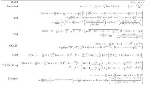
whereψ_≡ψ1. The integrals on the exponent can be computed analytically for several L´evy models,

see Table2, using any symbolic computation package such as Mathematica. Under the measureP_,

¯

φt,z,T(u, υ) =E[exp{iu(Xt+Xz−2XT) +iυ(YT−XT)}]

= exp

−rT+

Z T

0

ψ₋u(1[t∧z,T](s) +1[t∨z,T](s))−υ

s T −i

ds

(24)

holds.

In the case of the ASV models considered in this study, obtaining the characteristic functions based on the continuous average by applying the same limiting argument as in the L´evy model case on the discrete average-based characteristic functions (16) and (19) is not trivial. Alternatively, it is necessary to derive first the characteristic function of the triple (V, X, Y) (see [47] for the case of ASV models). Given this and by iterated expectations, we can then obtain expressions for the characteristic functions of (Xt+Xz, YT) under the risk neutral measure and (Xt+Xz−2XT, YT−

XT) under the measureP.

Finally, in the case of the CEV diffusion, the continuous-time analogues of (20) and (21) are given by

E

e−µ(Y_T−Yt)

Ft

= expnϕT−t

µ

T,0

−ψT−t

µ

T,0

Xt

o

(25)

(see [51, Proposition 6.2.4]) and

E

X

1 2−γ

t e−µYT

=X

1 2−γ 0 exp

n

rt+ϕT−t

µ

T,0

+ ¯ϕt

µ

T, ψT−t

µ

T,0

−ψt

µ

T, ψT−t

µ

T,0

X0

o

(26)

which follows from (25) by iterated expectations and a change to the measureP_{withϕ, ψ,ϕ¯ given}

by (10), (11), (22).

3.1. Lower bounds for discrete Asian options. In the case of the discrete average, the payoff of the arithmetic Asian call option with time to maturityT has form

PN

k=0S∆k

N+ 1 −KS¯ ∆N−K

!+

≡

PN

k=0S∆k

N+ 1 −KS¯ ∆N−K

!

1A (27)

consisting of the fixed strike price K_≥0 and coefficient ¯K_≥0 for floating strike options, with

A_≡

1 N+ 1

XN

k=0S∆k>

¯

KS∆N+K

. (28)

The time-0 value of this option,P0, satisfies

P0=e−rTE

" _PN

k=0S∆k

N+ 1 −KS¯ ∆N−K

! 1A

#

≥LB0≡e−rTE

" _PN

k=0S∆k

N+ 1 −KS¯ ∆N−K

! 1A′

#

for any A′_{⊂Ω as} 1 N+1

PN

k=0S∆k≤KS¯ ∆N+K in A

′ _{\ A. Therefore, the value of the option with} fixed strike (i.e.,K >0,K¯ = 0) or floating strike (i.e., K= 0,K >¯ 0) satisfies respectively

Pfix,0 ≥ LBfix,0=e−rTE

" _PN

k=0S∆k

N+ 1 −K

! 1A′

#

, (29)

Pfl,0 ≥ LBfl,0=e−rTE

"

S∆N

PN

k=0S∆kS∆−1N

N+ 1 −K¯

! 1A′

#

=S0E

" _PN

k=0S∆kS∆−1N

N+ 1 −K¯

! 1A′

#

, (30)

where the last equality in (30) follows by a change to theP_measure.

Thus, the choice of a A′ _{gives us a lower bound for the option price. The idea is that the chosen} A′ _{relates as closely as possible to the true A, so that the distance between the lower bound and} the true option price is minimized, while at the same time makes the problem more analytically tractable compared to the originalA. In what follows, we explain howA′ _{is determined depending} on the model choice for the underlying asset price dynamics. For consistency with (29) and (30), we define a parameterm taking value 0 (1) in the case of the fixed (floating) strike option.

3.1.1. The case of L´evy and ASV models. Given that

1 N+ 1

XN

k=0S∆kS

−m ∆N ≥

YN

k=0S∆kS

−m ∆N

1/(N+1)

(31)

(e.g., see [1, _§3.2.1]), we choose

A′ ≡

(

YN

k=0S∆kS

−m ∆N

1/(N+1)

>exp(λ)

)

≡

1 N+ 1

XN

k=0lnS∆k−mlnS∆N> λ

(32)

3.1.2. The case of the CEV diffusion model. CEV diffusion is treated separately from L´evy and ASV models as of interest in this case is the quantity 1

N+1

PN

k=0(S∆kS∆N−m)2−γ with useful

distributional properties, as opposed to 1 N+1

PN

k=0S∆kS∆N−m. Inequalities

1 N+ 1

XN

k=0S∆kS

−m ∆N ≷

1 N+ 1

XN

k=0(S∆kS

−m ∆N)

2−γ

1/(2−γ)

(33)

which hold for γ≷1 (e.g., see [1, _§3.2.4]) motivate the following choice ofA′ _{forλ >0}

A′_≡

  

1 N+ 1

XN

k=0

S∆k

Sm

∆N

2−γ!2−1γ

> λ2−1γ

   ≡ 1 N+1 PN k=0

S∆k

Sm

∆N

2−γ

> λ

1{γ<1} ∪ 1 N+1 PN k=0

S∆k

Sm

∆N

2−γ

> λ

1{1<γ<2} ∪ 1 N+1 PN k=0

S∆k

Sm

∆N

2−γ

< λ

1{γ>2}

. (34)

The averages 1 N+1

PN

k=0S∆kS∆N−m and 1 N+1

PN

k=0(S∆kS∆N−m)2−γ are positively correlated for γ <2,

whereas the correlation becomes negative forγ >2.

3.2. Lower bound optimization and transform representations for discrete Asian options. Due to the correlation between the two types of average, i.e., 1

N+1

PN

k=0S∆kS∆N−m and 1

N+1

PN

k=0ln(S∆kS∆N−m) for L´evy and ASV models orN1+1

PN

k=0S∆kS∆N−mandN1+1

PN

k=0(S∆kS∆N−m)2−γ

for the CEV model, by replacingAbyA′ _{and additionally optimizing the parameterλwe minimize} the error in the lower bound. In Section4 we prove an estimate for the error, whereas in Section

5 we demonstrate the effect of the optimal parameter λ in various numerical examples. Next, we determine the value of parameterλwhich maximizes the lower bounds (29) and (30).

Theorem 1. (Optimality conditions).Consider the random variablesY∆N =_N+11

PN

k=0X∆k

and Y¯∆N, where X= lnS, Y¯∆N ≡Y∆N−X∆N under L´evy and ASV models, and X=S2−γ,Y¯∆N≡

Y∆NX∆N−1 under the CEV diffusion. Then, the optimal lower bound is given for

λ∗

≡arg max

λ

LB0(λ)

which satisfies the optimality conditions

E PN

k=0S∆k

N+ 1

Y∆N =λ∗

!

=K and E PN

k=0S∆kS∆N−1

N+ 1

¯

Y∆N =λ∗

!

= ¯K, (35)

respectively, for a fixed and a floating strike option under L´evy, ASV and the CEV models.

Proof. We consider the case of the fixed strike option (the floating strike case is proved similarly). From (29) and the definitions of A′ _{given in (32) and (34)}

E

" _PN

k=0S∆k

N+ 1 −K

!

1{Y_∆N>λ}

#

= 1

N+ 1

XN

k=0

E_[E_{[S∆k−K|Y∆N]1{Y}

∆N>λ}]

(note that opposite inequality sign applies for CEV elasticity γ >2). Differentiating w.r.t. λ and interchanging with the expectation yields

1 N+ 1

XN

k=0 E

E_{[S∆k−K|Y∆N]} d

dλ1{Y∆N>λ}

= −1 N+ 1

XN

k=0

E_{(S∆k−K|Y∆N=λ)fN(λ), (36)}

where the last equality follows from d1{Y_∆N>λ}/dλ=−δ(Y∆N−λ) with δ representing the Dirac

delta function and fN the density function of Y∆N under the risk neutral measure. Then (35)

We now proceed to derive the transform representations of the lower bounds (29) and (30) with respect toλ, which can then be inverted to retrieve the lower bounds.

Theorem 2. (Fixed and floating strike discrete Asian options).

(i) (L´evy and ASV models). Suppose X= lnS. The Fourier transform of the lower bound (29) w.r.t.λ is

Φ(u;δ) _≡

Z

R

eiuλ+δλ

e−rT

N+ 1

XN

k=0

E_[(eX∆k_−K)1

{Y∆N>λ}]

dλ

= e

−rT

iu+δ

1 N+ 1

XN

k=0φk,k,N(−i/2, u−iδ)−KφN,N,N(0, u−iδ)

, (37)

where constant δ >0 ensures integrability and φ is given in (14) and (16), respectively, for L´evy and ASV models.

The Fourier transform of the lower bound (30) w.r.t. λis

¯

Φ(u;δ) _≡

Z

R

eiuλ+δλ

eX0

N+ 1

XN

k=0

E_[(eX∆k−X∆N_−K¯₎₁

{Y∆N−X∆N>λ}]

dλ

= e

X0

iu+δ

1 N+ 1

XN

k=0

¯

φk,k,N(−i/2, u−iδ)−K¯φ¯N,N,N(0, u−iδ)

, (38)

whereφ¯is given in (18) and (19) for the relevant model cases.

(ii) (CEV model). Suppose X=S2−γ_{. The (bilateral) Laplace transform of the lower bound}

(29) w.r.t.λ is

Φ(iµ;δ) _≡

Z

R

e−µλ+δλ

e−rT

N+ 1

XN

k=0 E

h

(X_∆k1/(2−γ)₋K)1{Y∆N≷λ}

i

dλ

= sgn(δ)e −rT

−µ+δ

1 N+ 1

XN

k=0

Eh_X1/(2−γ)

∆k e

−(µ−δ)Y_∆Ni

−KE_[e−(µ−δ)Y∆N_]

, (39)

whereµ_∈iR_{, constantδ≷0forγ≶2,sgndenotes the signum function and}Eh_X1/(2−γ)

∆k e−(µ−δ)Y∆N

i

and E_[e−(µ−δ)Y_{∆N] are given in (21) and (20), respectively.}

The (bilateral) Laplace transform of the lower bound (30) w.r.t. λis

¯

Φ(iµ;δ)≡

Z

R

e−µλ+δλ

(

X01/(2−γ)

N+ 1

XN

k=0

Eh_((X∆kX−1 ∆N)1

/(2−γ)_{−K)¯ 1}

{Y∆NX∆−N1≷λ}

i )

dλ

= sgn(δ)X

1/(2−γ) 0

−µ+δ

₁

N+ 1

XN

k=0

Eh_(X∆kX−1 ∆N)

1/(2−γ)_e−(µ−δ)Y∆NX∆−N1

i

−K¯E_[e−(µ−δ)Y∆NX∆−N1]

, (40)

where the expected values in (40) are computed numerically1_.

(iii) The lower bounds (29) and (30) are given in terms of the inversion formulae

LBfix,0(λ) =

e−δλ

2π

Z

R

e−iuλΦ(u;δ)du and LBfl,0(λ) =

e−δλ

2π

Z

R

e−iuλΦ(¯ u;δ)du, (41)

whereΦ(resp. Φ¯) is given in (37) (resp.38) for L´evy and ASV models and (39) (resp.40) for the CEV model.

1_{Derivation of explicit expressions for the expected values in (40) is not trivial. Instead, in principle, these can}

Proof. See Appendix A.

Remark 1 (Price sensitivities). One of the advantages of our method is that, at essentially no additional computational cost, it lends itself to computing the option price sensitivity with respect to some parameterκof interest, e.g., the initial value or volatility of the underlying asset, the risk-free rate, etc. This is possible: (i) assuming that the interchange of differentiation and integration in (41) is allowed, a usual assumption in option pricing via Fourier transform; and (ii) resorting to the envelope theorem2 _{(see [66, p. 160]). For example, in the case of the fixed strike}

Asian option we compute the price sensitivities by

∂LBfix,0(λ∗;κ)

∂κ =

e−δλ∗

2π

Z

R

e−iuλ∗∂Φ(u;δ, κ)

∂κ du, (42)

whereλ∗ _{satisfies (35) (we change slightly our notation here to make explicit the dependence of Φ} and, hence, LBfix,0 onκ). We highlight that (42) is the derivative of the lower bound for the option

price in (41) w.r.t. κ and does not imply a bound for the corresponding sensitivity. By sake of exemplification, to compute the delta we require

∂Φ (u;δ, X0)

∂S0

=∂Φ (u;δ, X0) ∂X0

∂X0

∂S0

,

where ∂Φ (u;δ, X0)/∂X0 is computed using (37) and (14) for L´evy models; (37) and (16) for ASV

models; (39) and (20)–(21) for the CEV model. In addition, ∂X0/∂S0= exp(−X0) for L´evy and

ASV models;∂X0/∂S0= (2−γ)X0−1 for the CEV model.

Based on the same principles, gamma can be computed by the second derivative of (41) w.r.t. S0.

Remark 2 (Australian options). It is worth noting that our construction can be adapted easily to the case of Australian options, i.e., options whose payoff depends on 1

N+1

PN

k=0S∆kS

−1 ∆N

(e.g., see [36]). Pricing in this case is similar to that of floating strike options (see expression 30, however with the expected values taken under the risk neutral measure andS0 replaced by e−rT).

3.3. Lower bounds for continuous Asian options. The results for the continuous average case are derived with a straightforward application of the same passages as in Section3.1. In more details,

e−rT_E

" ₁

T

Z T

0

Stdt−K

+#

≥e−rT_E

₁

T

Z T

0

Stdt−K

1{YT>λ}

, (43)

e−rT_E

" ST 1 T Z T 0

StST−1dt−K¯

+#

≥S0E

1 T

Z T

0

StST−1dt−K¯

1{Y¯T>λ}

, (44)

where YT =_T1

RT

0 Xtdt, ¯YT ≡YT−XT under L´evy and ASV models, ¯YT ≡YTX

−1

T under the CEV

diffusion. Note that opposite inequality sign applies in the indicator functions in (43)–(44) for CEV elasticityγ >2. The maximum lower bounds are given forλ=λ∗ _satisfying

E 1 T Z T 0

Stdt

YT =λ∗

=K andE

1 T

Z T

0

StST−1dt

¯ YT =λ∗

= ¯K. (45)

2_{Changes in the parameters may cause changes in the optimal valueλ}∗_{in Theorem1and the maximum lower bound}

Theorem 3. (Fixed and floating strike continuous Asian options).

(i) (L´evy and ASV models). Suppose X= lnS. The Fourier transform of the lower bound (43) w.r.t.λ is

Φ(u;δ) _≡

Z

R

eiuλ+δλ

e−rT

T

Z T

0

E_[(eXt_−K)1

{Y_T>λ}]dt

dλ

= e −rT

iu+δ

1 T

Z T

0

φt,t,T(−i/2, u−iδ)dt−KφT,T,T(0, u−iδ)

, (46)

where constant δ >0 ensures integrability and φ is given in (23) for L´evy models. The Fourier transform of the lower bound (44) w.r.t. λis

¯

Φ(u;δ) _≡

Z

R

ei(u−iδ)λ

eX₀

T

Z T

0

E_[(eXt−XT _−K)1

{Y_T−X_T>λ}]dt

dλ

= e

X0

iu+δ

1 T Z T 0 ¯

φt,t,T(−i/2, u−iδ)dt−Kφ¯T,T,T(0, u−iδ)

, (47)

whereφ¯is given in (24) for L´evy models3_.

(ii) (CEV model). Suppose X=S2−γ_{. The (bilateral) Laplace transform of the lower bound}

(43) w.r.t.λ is

Φ(iµ;δ) _≡

Z

R

e−µλ+δλ

e−rT

T

Z T

0

Eh_(X1/(2−γ)

t −K)1{YT≷λ}

i

dt

dλ

= sgn(δ)e −rT

−µ+δ

1 T

Z T

0

Eh_Xt1/(2−γ)_e−(µ−δ)YT

i

dt₋KE_[e−(µ−δ)YT_]

, (48)

whereµ_∈iR_{, constant δ≷0 forγ≶2, sgndenotes the signum function and} Eh_Xt1/(2−γ)_e−(µ−δ)Y_Ti

and E_[e−(µ−δ)YT_{]are given in (26) and (25), respectively.}

The (bilateral) Laplace transform of the lower bound (44) w.r.t. λis

¯

Φ(iµ;δ)_≡

Z

R

e−µλ+δλ

(

X₀1/(2−γ) T

Z T

0

Eh_((XtX−1 T )

1/(2−γ)

−K¯)1_{Y

TXT−1≷λ}

i

dt

)

dλ

= sgn(δ)X

1/(2−γ) 0

−µ+δ

1 T Z T 0 E h

(XtXT−1)

1/(2−γ)_e−(µ−δ)YTXT−1

i

dt₋K¯E_[e−(µ−δ)YTXT−1]

. (49)

(iii) The lower bounds (43) and (44) are given in terms of the inversion formulae

LBfix,0(λ) =

e−δλ

2π

Z

R

e−iuλ_{Φ(u;δ)du and LB}

fl,0(λ) =

e−δλ

2π

Z

R

e−iuλ_{Φ(¯ u;δ)du, (50)}

whereΦ and Φ¯ are given in (46)–(49) for the relevant models and types of options. Proof. The proof proceeds along the same lines as that of Theorem2.

The option price sensitivities can be obtained as explained in Remark 1.

Remark 3 (Generalized weighted sums). It is worth noting that our lower bound results can be extended to payoffs which depend on some generalized weighted sum of asset prices

RT

0 Stµ(t)dt, where µ(t) represents a measure on the time interval [0, T] on which we monitor the

underlying asset price process; this encompasses the cases of the continuous Asian option with µ(t)_≡ 1

T and discrete Asian option withµ(t)≡ 1 N+1

PN

k=0δ(∆k)(t) whereδ denotes the Dirac delta.

Our lower bound results are readily extendible to other candidates forµ of interest.

4. An estimate for the error of the lower bound. In what follows, we derive an estimate, in the form of an upper bound, for the error when approximating the true Asian option price using the general lower bound of Section 3 based on the principles set out in Rogers and Shi [61] and Nielsen and Sandmann [58] in the Gaussian model setting and Lemmens et al. [52] under L´evy models.

Theorem 4. (Error bounds). Consider the random variables Y∆N = _N1₊₁

PN

k=0X∆k and

¯

Y∆N, whereX= lnS, Y¯∆N =Y∆N −X∆N under L´evy and ASV models, and Y¯∆N=Y∆NX∆N−1 with

X=S2−γ _{under the CEV diffusion. In addition,Y} T =_T1

RT

0 Xtdtand Y¯T =YT−XT orY¯T=YTX

−1 T

for the relevant model case.

(i) (Discrete average, fixed and floating strike options). The error ǫ from approxi-mating the price of the Asian call option on the discrete average with payoff (27) for a fixed strike (i.e., K >0,K¯ = 0) or a floating strike (i.e., K= 0,K >¯ 0) by the corresponding lower bound (29) or (30) is bounded, respectively, by

0 ≤ǫfix≤

e−rT

2(N+ 1)E

( XN

k,n=1

E_{(S∆kS∆n|Y∆N)−}XN

k=1

E_{(S∆k|Y∆N)} 212

1{Y∆N≤λ∗}

)

, (51) 0 ≤ǫfl≤

S0

2(N+ 1)E

( XN

k,n=1

E_(S∆kS∆nS−2

∆N|Y¯∆N)−

XN k=1

E_(S∆kS−1 ∆N|Y¯∆N)

2

1 2

1{Y¯∆N≤λ∗}

)

,(52)

where the expectations in (51) and (52) are taken under the P _and P _{measures, respectively.} (ii) (Continuous average, fixed and floating strike options).The error from approx-imating the price of the fixed or floating strike Asian call option on the continuous average by the corresponding lower bound (43) or (44) is bounded, respectively, by

0_≤ ǫfix≤

e−rT

2T E

   " Z [0,T]2

E_{(StSz|YT)d(t, z)−}

Z T

0

E_(St|YT)dt 2#

1 2

1{Y_T≤λ∗}

 



, (53)

0_≤ ǫfl≤

S0

2TE

 

 "

Z

[0,T]2

E_(StSzS−2

T |Y¯T)d(t, z)−

Z T

0

E_(StS−1 T |Y¯T)dt

2# 1 2

1{Y¯_T≤λ∗}

 



, (54)

where the expectations in (53) and (54) are taken under the P _and P _{measures, respectively.} (Note that for CEV elasticity γ >2, the inequality sign in the indicator functions in (51)–(54) is reversed.)

Proof. See Appendix A.

From (51)–(54) (see also 67) it is obvious that the more information the conditioning average contains about the original arithmetic average, the smaller the conditional variance of the arith-metic average, hence the smaller the error in the lower bound price approximation, becomes. This confirms our choice of the conditioning average and of A′ _{to substitute forA in Section3.}

It is possible to obtain analytical expressions for the error bounds (51) and (52). More specifically, we get

E_(S∆kS∆nm _{|Y∆N=y) =} R

Re

−iυy_E(S

∆kS∆nm eiυY∆N)dυ

R Re

−iυy_E(eiυY_∆N)dυ , (55)

E_(S∆kSm ∆nS

−1−m

∆N |Y¯∆N=y) =

R Re

−iυy_E(S

∆kS∆nm S

−1−m ∆N eiυ

¯ Y_∆N)dυ

R Re

−iυyE_(eiυY¯∆N)dυ (56) form= 0,1 (see [7, p. 62–63]). Consider the functionsφand ¯φgiven respectively by the expressions (14) and (18) for X driven by a L´evy model; (16) and (19) for X driven by an ASV model. Then, we have that

E_(S∆kSm ∆ne

iυY∆N_{) = φ}

E_(S∆kSm ∆nS

−1−m ∆N e

iυY¯∆N_{) = ¯φ}

k,m(n−k)+k,N(−i/(2−m), υ), E_(eiυY∆N_{) =φ}

N,N,N(0, υ) and E(eiυ ¯

Y_{∆N) = ¯φ}

N,N,N(0, υ).

In the case of the CEV model, form= 0

E_(S∆keiυY∆N_{) =}E_(X∆k1/(2−γ)_eiυY∆N_{) and}E_(eiυY∆N₎

are given explicitly in (21) and (20), whereas the remaining expected values in (55)–(56) can be computed numerically or using fractional calculus techniques as 1/(2₋γ)_∈R_{, see Cressie and}

Borkent [26], subject to certain regularity conditions.

In the case of the continuous average, the error bounds (53) and (54) can also be computed by means of explicit conditional expectation representations, similar to (55)–(56) for the discrete aver-age, to the extent these are available for different model specifications under continuous averaging: for example, see (23)–(24) for L´evy models; (25)–(26) for the CEV model; discussion in Section2.5

for ASV models.

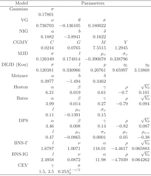
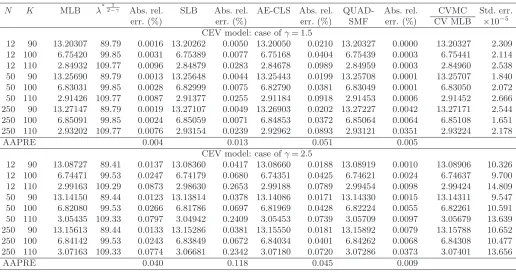
5. Numerical study. In order to illustrate the performance of our maximum lower bound (MLB) with optimal parameter λ=λ∗ _{satisfying (35) or (45), respectively for a discrete or a} continuous average, we perform an extensive pricing exercise across a wide range of stochastic dynamic models (see Table 3) for varying strike price K and monitoring frequency. In addition, we consider a suboptimal lower bound (SLB) in which we fix the parameter λ= lnK, for L´evy and ASV models, andλ=K2−γ_{, for the CEV diffusion; these choices follow from a comparison of}

A given in (28), based on the original average, and A′ _{in (32) and (34), based on the correlated} average. (In the case of floating strike options, K should be replaced by ¯K.) Formulae (41) and (50), respectively for a discrete and a continuous average, are computed using the (fractional) fast Fourier transform algorithm (e.g., fftorczt in Matlab, see [21] for more details) which outputs: (i) lower bound values on a fine, equally spaced grid of parameter λ values, including the MLB for optimal λ=λ∗ _{as well as the SLB for λ= lnK or λ=K}2−γ_{; and (ii) the optimal value λ}∗_. Computed lower bounds are then compared with benchmark prices generated by a very accurate control variate Monte Carlo (CVMC) simulation method using as control variates the lower bounds themselves4_{; we call these optimized CVMC (with the MLB as CV) and suboptimal CVMC (with}

the SLB as CV). We employ CVMC setup with the CV coefficient estimated in a pilot run, e.g., see Glasserman [43] and Cont and Tankov [23]. The choice of the CVMC method is justified by its high accuracy and applicability under various model assumptions for the underlying asset price process. In AppendixB, we summarize the simulation methodologies we have used in our numerical study. Note that when estimating the price of the option on the continuous average, we correct the discretization bias inherent in the simulation using our maximum lower bound based on the continuous average as the control variate5_{. The sets of parameter values used for the L´evy models}

are from the calibrations of Schoutens [62] and Fusai and Meucci [40]; the ASV models’ parameter values are from the calibrations of Duffie et al. [33] (see also [13], [2] and [68]) and Nicolato and Venardos [57]; the CEV parameter sets are taken from Cai et al. [15].

In addition, where applicable, we compare with numerical results from other important methods in the literature, including, for example, Geman and Yor [42], Zhang [74], Dewynne and Shaw [31], Cai and Kou [14], Bayraktar and Xing [9], Ewald et al. [36], Cai et al. [15] and Sesana et al.

4_{Lower bound price approximations have also been used as control variates in Caldana and Fusai [17] in simulating}

spread option prices with substantial variance reduction effect.

5_{Fu et al. [37] have implemented previously a similar efficient simulation approach for pricing continuous arithmetic}

[64]. We point out that the relevant results consist of various model settings for the underlying, parameter values for the volatility, interest rate and dividend yield, contract parameters such as the strike price, and monitoring frequencies (discrete and continuous).

Our computations are conducted on a desktop PC with an Intel Core 2 Duo 2.93 GHz processor and 2.00 GB of RAM. As our computing platforms, we have chosen Matlab R2010a and, for the method of Bayraktar and Xing [9], Visual C++ 2010.

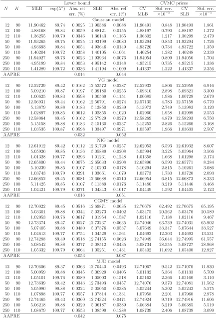
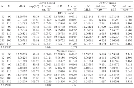
5.1. Performance comparisons against Monte Carlo simulation benchmarks. First, we consider the case of the discrete average. Tables 4–5 give numerical results of prices of Asian options under various L´evy models (Gaussian, VG, NIG, CGMY, MJD, DEJD, Meixner) and ASV models (Heston, Bates, DPS, BNS-Γ, BNS-IG). We let the strike vary from 90 to 110 with an increment of 10 and consider different monitoring frequencies: monthly (N= 12), weekly (N= 50) and daily (N = 250). It can be seen that the optimized CVMC systematically produces estimates with lower standard errors than the suboptimal CVMC. For this, in what follows we consider only the optimized CVMC estimates. In fact, our reported optimized CVMC price estimates are accurate to 4₋5 decimal places (at the 95% confidence level), hence can serve as benchmarks to the numerical outcomes from alternative pricing methods. However, despite its high accuracy, Monte Carlo simulation can be computationally intensive, in general, for high monitoring frequencies, but also in model-specific cases, such as the Meixner, Bates, BNS-Γ and BNS-IG models, by construction of their simulation procedures with CPU times in excess of 1000 seconds per price estimate forN= 12. A comparison in terms of the average absolute % relative error (AAPRE) of the MLB and SLB against the optimized CVMC estimates across strikes and number of monitoring dates indicates that the MLB generates AAPREs in the range 0.01%₋0.05% under the L´evy models and 0.02%₋0.03% under stochastic volatility, whereas the SLB produces AAPREs of 0.04%₋0.09% and 0.1%₋0.16% respectively. In summary, Tables 4–5 suggest that the MLB is consistently more accurate and robust than the SLB across different models, contract specifications and monitoring frequencies. More importantly, given its high accuracy level and ease of use, the MLB can be used itself as an efficient and power-saving substitute to the CVMC price.

In Table 6, we extend our analysis to the CEV asset price model. More specifically, we compare our MLB and SLB results for different elasticitiesγ with those obtained through the quadrature method of Sesana et al. [64] and the asymptotic expansion approach of Cai et al. [15]. Based on the AAPREs computed against the optimized CVMC estimates, the SLB is shown to perform consistently worse than the MLB. It can be seen that for γ= 1.5 the MLB produces the lowest AAPRE and also the lowest maximum absolute % relative error (MAPRE), i.e., 0.004% (0.009%), followed by the quadrature method with 0.005% (0.035%), the SLB with 0.013% (0.028%) and the expansion formula with 0.051% (0.098%); for γ = 2.5, the AAPREs (MAPREs) are found to be 0.009% (0.037%), 0.040% (0.087%), 0.045% (0.078%), 0.118% (0.265%), respectively, for the quadrature method, the MLB, the expansion formula and the SLB. Although very accurate, the quadrature method by Sesana et al. [64] turns out be computationally expensive requiring approximately 90 seconds, as opposed to 0.15 seconds required by our MLB, forN= 12, with the CPU times further increasing withN. On the other hand, the expansion formula of Cai et al. [15] is very fast, generating one result in less than 0.5 seconds almost independently of N, however its applicability is limited to one-dimensional diffusion models.

our method also in this computation: for example, this generates AAPRE of 0.005% under CEV with γ= 1.5, which is an improvement to the asymptotic expansion approach of Cai et al. [15] with AAPRE of 0.028% in this case, whereas both methods perform the same under CEV with γ= 2.5 with AAPRE of 0.013%. Our approximation seems less accurate in the case of the gamma sensitivity (still acceptable for practical applications) with AAPRE of 0.5% (approx.) for both γ= 1.5,2.5.

Next, we assess the performance of our MLB in the case of the continuous average. In light of recent advances on the pricing of continuous Asian options, we compare with the numerical prices from the inversion of the double-Laplace transform of Cai and Kou [14] under the DEJD model; the PIDE implementation of Bayraktar and Xing [9] under the MJD and DEJD models; and the implementation of the PDE developed in Ewald et al. [36], as well as the second-order Taylor 2.0 Monte Carlo price estimates of Ewald et al. [36] under the Heston model. A more detailed analysis under the Gaussian model dynamics is deferred to Section5.2. Using the same sets of parameters as in the aforementioned works, it is shown in Table8that the MLB and the double-Laplace transform algorithm generate nearby AAPREs under the DEJD model with jump arrival rate l= 3 (l= 5), i.e., 0.02% and 0.01% (0.03% and 0.06%), as opposed to the PIDE method of Bayraktar and Xing [9] with a persistently higher AAPRE of 0.07% (0.15%). Also, the reported MAPREs follow the same pattern across the different methods. The CPU times per result are approximately 4, 6 and 6 seconds for the MLB, the double-Laplace transform algorithm and the PIDE method. Under the MJD model with l= 1, the PIDE method’s AAPRE improves to 0.03%, whereas the AAPRE of our MLB is only marginally affected and is no greater than 0.04%. In Table9, we present numerical results for continuous Asian options under the Heston model. Given the simulation error (RMSE) reports for the second-order Taylor scheme implemented in Ewald et al. [36], we reach that the relevant price estimates are accurate to 1₋2 decimal places (at the 90% confidence level) with each estimate taking 310 seconds to compute. In addition, implementing the PDE of Ewald et al. [36] takes approximately 1000 seconds to generate a price result accurate to 3 decimal places, whereas our MLB requires approximately 10 seconds for the same level of precision.

5.2. Pricing under the Gaussian model: comparisons for varying volatility. In this section, we focus attention on the special case of the continuous Asian option under the basic Gaussian model. To check the accuracy of our MLB, we adhere to the test cases considered in Cai and Kou [14] and compare against existing methods devoted to the Gaussian dynamics and the continuous average case.

Table 10 shows that in most of the cases of moderate to high volatility, 0.1_≤σ_≤0.5, our MLB results agree to 4 decimal places with the prices obtained from the methods of Geman and Yor [42], Linetsky [53], Cai and Kou [14] (accurate to 10 decimal places), and Veˇceˇr [69], Zhang [74] (accurate to 6 decimal places). Although the MLB seems less accurate than the other approaches (still suffi-ciently accurate for practical applications), its performance improves substantially with decreasing volatility to extremely low levels in which case many numerical methods for Asian options per-form poorly. Here, we extend the previous analysis of Cai and Kou [14] on cross-comparisons of behaviours for reasonably low volatilities, e.g., σ= 0.05, and extremely low volatilities, σ_≤0.01, to include also our MLB method. Further, we study different cases q < r,q=r, q > r. Table 11

In summary, our results confirm the efficiency of our MLB which becomes remarkably sharp at low volatility levels.

5.3. Upper bounds for Asian option prices. In Section 4, we have derived theoretical upper bounds to the error ǫfrom approximating the true option prices by the lower bounds (see Theorem 4). For the model cases of Tables 4–6, we report in Table 12 our upper error bounds computed numerically using the fast Fourier transform algorithm for (i) our maximum lower bound and (ii) the suboptimal lower bound; we call these optimized and suboptimal error bounds, respec-tively. Note that, when added to the lower bounds, these error estimates give us also access to upper bounds to the true option prices.

We observe that in all cases the optimized upper bounds are tighter than the suboptimal ones. It also appears that the error is an increasing function of the strike price, whereas the impact of increasing number of monitoring dates to the error is trivial; this is consistent with the results of Nielsen and Sandmann [58] based on a lognormal underlying asset price and an improvement over the more conservative upper bound of Rogers and Shi [61] which is independent of the strike price level. It is worth noting that the same behaviour across strikes and number of monitoring dates is observed also in the experimental absolute % relative errors reported in Tables4–6. In addition, the experimental relative differences between the reported MLBs and the benchmark CVMC estimates in Tables4–6across all strikes and monitoring dates are no greater than 0.0067 for the L´evy models, 0.0004 for the ASV models and 0.0026 for the CEV diffusion, whereas the corresponding computed theoretical error estimates presented in Table 12 appear higher (in particular, these are smaller than 0.2390, 0.054 and 0.148) in consistency with the theoretical analysis as the latter represent upper bounds to the true error.

6. Conclusions. In this paper, an approximation in the form of an acute lower bound is proposed to price discretely or continuously monitored Asian options, with fixed or floating strike price, in a general model setting with jumps allowed or not in the underlying asset returns and in the evolution of the volatility process. Special attention is given to the CEV diffusion model with distinct distributional properties. An estimate to the error from the lower bound approximation is also obtained. Extensive numerical experiments across a wide range of stochastic dynamic models, monitoring frequencies and option moneyness indicate that our proposed method is easy to imple-ment, fast and accurate compared to other important methods in the literature; and it performs remarkably well even in the case of extremely low volatilities.

We note that our approach can be applied to exponential L´evy-driven mean-reverting models, which, although we have only briefly mentioned in the paper, are nevertheless empirically accepted by several studies as important models for commodity price dynamics. Following a change to the forward measure, it can be also extended to the case of affine models with stochastic interest rates, which become more essential in the case of long-dated contracts. Finally, our approximation can be applied to in-progress options and functions of generalized weighted (discrete or continuous) sums of asset prices.

Appendix A: Proofs.

Proof of Proposition 1. From (1) we have that for any 0_≤a < b,

X∆b =X∆a+

Xb

j=a+1Z ∆

j , (57)

Xb

j=a+1X∆j = (b−a)X∆a+

Xb

j=a+1(b+ 1−j)Z ∆

hold. Based on (57)–(58) we are able to write

Y∆N =

1 N+ 1

XN

j=0X∆j=X0+

XN

j=1

1₋ j N+ 1

Zj∆, (59)

X∆(k∧n)+X∆(k∨n) = 2X0+ 2

Xk∧n

j=1Z ∆ j +

Xk∨n

j=k∧n+1Z ∆

j . (60)

Given thatX∆k+X∆n≡X∆(k∧n)+X∆(k∨n), we get from (59)–(60)

E_{[exp{iu(X∆k+X∆n) +iυY∆N}] =}E_{[exp{iu(X∆(k∧n)+X∆(k∨n)) +iυY∆N}]}

= exp_{i(2u+υ)X0}E

exp

iXk∧n

j=1

2u+υ

1₋ j N+ 1

Zj∆

+iXk∨n

j=k∧n+1

u+υ

1₋ j N+ 1

Z∆ j +i

XN

j=k∨n+1υ

1₋ j N+ 1

Z∆ j

.

(i) Given (2) and (13), (14) follows by stochastic independence ofZ∆ j .

(ii) From (6) we have

E_{[exp{ϑNV∆N+iηNZN}∆_{}|F∆(N−1)] = exp{ϕ∆(ϑN, iηN) +ψ∆(ϑN, iηN)V∆(N−1)} (61)}

and forj=N₋1, . . . , k_∨n, . . . , k_∧n, . . . ,1

E_{[exp{ψ∆(ϑj+1, iηj+1)V∆j+iηjZj}∆_{}|F∆(j−1)]}

= exp_{ϕ∆(ψ∆(ϑj+1, iηj+1), iηj) +ψ∆(ψ∆(ϑj+1, iηj+1), iηj)V∆(j−1)}

= exp_{ϕ∆(ϑj, iηj) +ψ∆(ϑj, iηj)V∆(j−1)}, (62)

where the last equality follows from (15). Then, given (59)–(60) and using iterated expectations applying (61)–(62), we obtain (16).

Proof of Proposition 2. Based on (57)–(58) we are able to write

Y∆N−X∆N =

1 N+ 1

XN

j=0X∆j−X∆N=

−1 N+ 1

XN

j=1jZ ∆

j , (63)

X∆(k∧n)+X∆(k∨n)−2X∆N = −

Xk∨n

j=k∧n+1Z ∆ j −2

XN

j=k∨n+1Z ∆

j . (64)

From (63)–(64) we get

E_{[exp{iu(X∆k+X∆n−2X∆N) +iυ(Y∆N−X∆N)}]}

=E_{[exp{iu(X∆(k∧n)+X∆(k∨n)−2X∆N) +iυ(Y∆N−X∆N)}]}

=E

exp

−iXk∧n

j=1υ

j N+ 1Z

∆ j

−iXk∨n

j=k∧n+1

u+υ j N+ 1

Z∆ j −i

XN

j=k∨n+1

2u+υ j N+ 1

Z∆ j

.

(i)–(ii) Given the arguments above, the proof follows that of parts (i)–(ii) of Proposition1using (4) and (7) instead of (2) and (6).