Faster Algorithms for Quantitative Verification in Constant Treewidth Graphs

Faster Algorithms for Quantitative Verification in Constant Treewidth

Graphs

Krishnendu Chatterjee† Rasmus Ibsen-Jensen† Andreas Pavlogiannis† †

IST Austria

Abstract. We consider the core algorithmic problems related to verification of systems with respect to three clas-sical quantitative properties, namely, the mean-payoff property, the ratio property, and the minimum initial credit for energy property. The algorithmic problem given a graph and a quantitative property asks to compute the optimal value (the infimum value over all traces) from every node of the graph. We consider graphs with constant treewidth, and it is well-known that the control-flow graphs of most programs have constant treewidth. Letndenote the number of nodes of a graph,mthe number of edges (for constant treewidth graphsm=O(n)) andWthe largest absolute value of the weights. Our main theoretical results are as follows. First, for constant treewidth graphs we present an algorithm that approximates the mean-payoff value within a multiplicative factor ofin timeO(n·log(n/))and linear space, as compared to the classical algorithms that require quadratic time. Second, for the ratio property we present an algorithm that for constant treewidth graphs works in timeO(n·log(|a·b|)) =O(n·log(n·W)), when the output isa

b, as compared to the previously best known algorithm with running timeO(n

2_{·log(n·W)).}

Third, for the minimum initial credit problem we show that (i) for general graphs the problem can be solved in O(n2_{·m)time and the associated decision problem can be solved inO(n·m)time, improving the previous known}

O(n3·m·log(n·W))andO(n2·m)bounds, respectively; and (ii) for constant treewidth graphs we present an algorithm that requiresO(n·logn)time, improving the previous knownO(n4·log(n·W))bound. We have implemented some of our algorithms and show that they present a significant speedup on standard benchmarks.

1

Introduction

Boolean vs quantitative verification.The traditional view of verification has beenqualitative (Boolean)that classifies traces of a system as “correct” vs “incorrect”. In the recent years, motivated by applications to analyze resource-constrained systems (such as embedded systems), there has been a huge interest to studyquantitativeproperties of systems. A quantitative property assigns to each trace of a system a real-number that quantifies how good or bad the trace is, instead of classifying it as correct vs incorrect. For example, a Boolean property may require that every request is eventually granted, whereas a quantitative property for each trace can measure the average waiting time between requests and corresponding grants.

Variety of results. Given the importance of quantitative verification, the traditional qualitative view of verifica-tion has been extended in several ways, such as, quantitative languages and quantitative automata for specificaverifica-tion languages [27,17,16,21,15,47,28]; quantitative logics for specification languages [8,10,2]; quantitative synthesis for robust reactive systems [4,5,20]; a framework for quantitative abstraction refinement [13]; quantitative analysis of infinite-state systems [22,18]; and model measuring (that extends model checking) [33], to name a few. The core al-gorithmic question for many of the above studies is a graph alal-gorithmic problem that requires to analyze a graph wrt a quantitative property.

time analysis [17,13,18]; the ratio property is used in robustness analysis of systems [5]; and the minimum initial credit for energy for measuring resource consumptions [9].

Algorithmic problems.Given a graph and a quantitative property, the value of a node is the infimum value of all traces that start at the respective node. The algorithmic problem (namely, thevalueproblem) for analysis of quantitative prop-erties consists of a graph and a quantitative property, and asks to compute either the exact value or an approximation of the value for every node in the graph. The algorithmic problems are at the heart of many applications, such as automata emptiness, model measuring, quantitative abstraction refinement, etc.

Treewidth of graphs.A very well-known concept in graph theory is the notion oftreewidthof a graph, which is a measure of how similar a graph is to a tree (a graph has treewidth 1 precisely if it is a tree) [44]. The treewidth of a graph is defined based on atree decompositionof the graph [31], see Section 2 for a formal definition. Beyond the mathematical elegance of the treewidth property for graphs, there are many classes of graphs which arise in practice and have constant treewidth. The most important example is that the control flow graphs of goto-free programs for many programming languages are of constant treewidth [45], and it was also shown in [30] that typically all Java programs have constant treewidth. For many other applications see the surveys [6,7]. The constant treewidth property of graphs has also played an important role in logic and verification; for example, MSO (Monadic Second Order logic) queries can be solved in polynomial time [?] (also in log-space [29]) for constant-treewidth graphs; parity games on graphs with constant treewidth can be solved in polynomial time [40]; and there exist faster algorithms for probabilistic models (like Markov decision processes) [14]. Moreover, recently it has been shown that the constant treewidth property is also useful for interprocedural analysis [18].

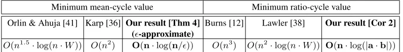
Minimum mean-cycle value Minimum ratio-cycle value

Orlin & Ahuja [41] Karp [36] Our result [Thm 4] (-approximate)

Burns [12] Lawler [38] Our result [Cor 2]

O(n1.5_{·log(n·W)) O(n}2_{) O(n·log(n/)) O(n}3_{) O(n}2_{·log(n·W)) O(n·log(|a·b|))}

Table 1: Time complexity of existing and our solutions for the minimum mean-cycle value and ratio-cycle value problem in constant treewidth weighted graphs withnnodes and largest absolute weightW, when the output is the (irreducible) fractiona_b 6= 0.

Bouyer et. al. [9] Our result [Thm 5, Cor 3]

Our result [Thm 7] (constant treewidth)

Time (decision) O(n2·m) O(n·m) O(n·logn) Time O(n3·m·log(n·W)) O(n2·m) O(n·logn)

Space O(n) O(n) O(n)

Table 2: Complexity of the existing and our solution for the minimum initial credit problem on weighted graphs ofn nodes,medges, and largest absolute weightW.

Previous results and our contributions.In this work we consider general graphs and graphs with constant treewidth, and the algorithmic problems to compute the exact value or an approximation of the value for every node wrt to quantitative properties given as the mean-payoff, the ratio, or the minimum initial credit for energy. We first present the relevant previous results, and then our contributions.

requiresO(n·m)running time andO(n2)space. A different algorithm was proposed in [39] that requiresO(n·m)

running time andO(n)space. Orlin and Ahuja [41] gave an algorithm running in timeO(√n·m·log(n·W)). For some special cases there exist faster approximation algorithms [19]. There is a straightforward reduction of the ratio problem to the mean-payoff problem. For computing the exact minimum ratio, the fastest known strongly polynomial time algorithm is Burns’ algorithm [12] running in timeO(n2_{·m). Also, there is an algorithm by Lawler [38] that}

usesO(n·m·log(n·W))time. Many pseudopolynomial algorithms are known for the problem, with polynomial dependency on the numbers appearing in the weight function, see [26]. For the minimum initial credit for energy problem, the decision problem (i.e., is the energy required for nodev at mostc?) can be solved inO(n2_·m)time,

leading to anO(n3_{·m·log(n·W))time algorithm for the minimum initial credit for energy problem [9]. All the}

above algorithms are for general graphs (without the constant-treewidth restriction).

Our contributions.Our main contributions are as follows.

1. Finding the mean-payoff and ratio values in constant-treewidth graphs. We present two results for constant treewidth graphs. First, for the exact computation we present an algorithm that requiresO(n·log(|a·b|))time and O(n)space, where a_b 6= 0is the (irreducible) ratio/mean-payoff of the output. If a_b = 0then the algorithm uses O(n)time. Note thatlog(|a·b|)≤2 log(n·W). We also present a space-efficient version of the algorithm that requires onlyO(logn)space. Second, we present an algorithm for finding an-factor approximation that requires O(n·log(n/))time andO(n)space, as compared to theO(n1.5_{·log(n·W))time solution of Orlin & Ahuja,}

and theO(n2_{)time solution of Karp (see Table 1).}

2. Finding the minimum initial credit in graphs.We present two results. First, we consider the exact computation for general graphs, and present (i) anO(n·m)time algorithm for the decision problem (improving the previous known O(n2_{·m)bound), and (ii) anO(n}2_{·m)time algorithm to compute value of all nodes (improving the}

previous knownO(n3_{·m·log(n·W))bound). Finally, we consider the computation of the exact value for graphs}

with constant treewidth and present an algorithm that requiresO(n·logn)time (improving the previous known O(n4_{·log(n·W))bound) (see Table 2).}

3. Experimental results.We have implemented our algorithms for the minimum mean cycle and minimum initial credit problems and ran them on standard benchmarks (DaCapo suit [3] for the minimum mean cycle problem, and DIMACS challenges [1] for the minimum initial credit problem). For the minimum mean cycle problem, our results show that our algorithm has lower running time than all the classical polynomial-time algorithms. For the minimum initial credit problem, our algorithm provides a significant speedup over the existing method. Both improvements are demonstrated even on graphs of small/medium size. Note that our theoretical improvements (better asymptotic bounds) imply improvements for large graphs, and our improvements on medium size graphs indicate that our algorithms have practical applicability with small constants.

Technical contributions.The key technical contributions of our work are as follows:

1. Mean-payoff and ratio values in constant-treewidth graphs.Given a graph with constant treewidth, letc∗be the smallest weight of a simple cycle. First, we present a linear-time algorithm that computesc∗exactly (ifc∗ ≥0) or approximate within a polynomial factor (ifc∗ <0). Then, we show that if the minimum ratio valueν∗is the irreducible fraction a_b, thenν∗can be computed by evaluatingO(log(|a·b|))inequalities of the formν∗ ≥ ν. Each such inequality is evaluated by computing the smallest weight of a simple cycle in a modified graph. Finally, for-approximating the valueν∗, we show thatO(log(n/))such inequalities suffice.

2

Definitions

Weighted graphs.We considerfinite weighted directed graphsG= (V, E,wt,wt0)whereV is the set ofnnodes, E⊆V ×V is the edge relation ofmedges,wt:E →_Zis aweight functionthat assigns an integer weightwt(e)to each edgee∈E, andwt0 :E →_N+_{is a weight function that assigns strictly positive integer weights. For technical}

simplicity, we assume that there exists at least one outgoing edge from every node. In certain cases where the function wt0is irrelevant, we will consider weighted graphsG= (V, E,wt), i.e., without the functionwt0.

Finite and infinite paths.Afinite pathP = (u1, . . . , uj), is a sequence of nodesui ∈V such that for all1≤i < j

we have(ui, ui+1) ∈ E. ThelengthofP is|P| = j−1. A single-node path has length0. The pathP issimple

if there is no node repeated in P, and it is a cycleif j > 1 andu1 = uj. The pathP is asimple cycle if P is

a cycle and the sequence (u2, . . . uj)is a simple path. The functionswtandwt0 naturally extend to paths, so that

the weight of a pathP with|P| > 0wrt the weight functions wtandwt0 iswt(P) = P

1≤i<jwt(ui, ui+1)and

wt0(P) =P

1≤i<jwt

0_(u

i, ui+1). ThevalueofP is defined to bewt(P) =

wt(P)

wt0_(P). For the case where|P|= 0, we definewt(P) = 0, andwt(P)is undefined. Aninfinite pathP = (u1, u2, . . .)ofGis an infinite sequence of nodes

such that every finite prefixPofPis a finite path ofG. The functionswtandwt0assign toPa value inZ∪ {−∞,∞}:

we havewt(P) = P

iwt(ui, ui+1)andwt0(P) =∞. For a (possibly infinite) pathP, we use the notationu∈Pto

denote that a nodeuappears inP, ande∈Pto denote that an edgeeappears inP. Given a setB ⊆V, we denote withP∩Bthe set of nodes ofB that appear inP. Given a finite pathP1and a possibly infinite pathP2, we denote

withP1◦P2the path resulting from the concatenation ofP1andP2.

Distances and witness paths.For nodesu, v∈V, we denote withd(u, v) = infP:u vwt(P)thedistancefromuto

v. A finite pathP :u vis awitnessof the distanced(u, v)ifwt(P) =d(u, v). An infinite pathP is a witness of the distanced(u, v)if the following conditions hold:

1. d(u, v) =wt(P) =−∞, and

2. P starts fromu, andvis reachable from every node ofP.

Note thatd(u, v) =∞is not witnessed by any path.

Tree decompositions.Atree-decompositionTree(G) = (VT, ET)ofGis a tree such that the following conditions

hold:

1. VT ={B0, . . . , Bn0₋₁:∀i B_i⊆V}andS_B

i∈VTBi=V (every node is covered).

2. For all(u, v)∈Ethere existsBi∈VT such thatu, v∈Bi(every edge is covered).

3. For alli, j, ksuch that there is a bagBkthat appears in the simple pathBi BjinTree(G), we haveBi∩Bj⊆

Bk(every node appears in a contiguous subtree ofTree(G)).

The setsBiwhich are nodes inVT are calledbags. Conventionally, we callB0the root ofTree(G), and denote with

Lv(Bi)the level of Bi inTree(G), withLv(B0) = 0. We say thatTree(G)is balancedif the maximum level is

maxBiLv(Bi) =O(logn

0_{), and it isbinaryif every bag has at most two children bags. A bagBis called theroot bag} of a nodeuifBis the smallest-level bag that containsu, and we often useButo refer to the root bag ofu. Thewidth

of a tree-decompositionTree(G)is the size of the largest bag minus1. The treewidth ofGis the smallest width among the widths of all possible tree decompositions ofG. The following lemma gives a fundamental structural property of tree-decompositions.

Lemma 1. Consider a graphG= (V, E), a binary tree-decompositionT = Tree(G)and a bagBofT. Denote with (Ci)1≤i≤3the components ofT created by removingB fromT, and letVibe the set of nodes that appear in bags of

componentCi. For everyi6=j, nodesu∈Vi,v∈VjandP :u v, we have thatP∩B6=∅(i.e., all paths between

uandvgo through some node inB).

In the sequel we consider only balanced and binary tree-decompositions of constant width andn0 =O(n)bags (and hence of heightO(logn)). Additionally, we consider that every bag is the root bag of at most one node. Obtaining this last property is straightforward, simply by replacing each bagB which is the root ofk >1 nodesx1, . . . xk with a

chain of bagsB1, . . . , Bk =B, where eachBiis the parent ofBi+1, andBi+1=Bi∪ {xi+1}. Note that this keeps

the tree binary and increases its height by at most a constant factor, hence the resulting tree is also balanced.

Throughout the paper, we follow the convention that the maximum and minimum of the empty set is −∞and∞ respectively, i.e., max(∅) = −∞ andmin(∅) = ∞. Time complexity is measured in number of arithmetic and logical operations, and space complexity is measured in number of machine words. Given a graphG, we denote with T(G)andS(G)the time and space required for constructing a balanced, binary tree-decompositionTree(G). We are interested in the following problems.

The minimum mean cycle problem [36].Given a weighted directed graphG= (V, E,wt), the minimum mean cycle problem asks to determine for each nodeuthemean valueµ∗(u) = minC∈Cu

wt(C)

|C| , whereCuis the set of simple

cycles reachable fromuinG. A cycleCwithwt_|C(C_|) =µ∗(u)is called a minimum mean cycle ofu. For0 < <1, we say that a valueµis an-approximation of the mean valueµ∗(u)if|µ−µ∗(u)| ≤· |µ∗_(u)|.

The minimum ratio cycle problem [32].Given a weighted directed graphG= (V, E,wt,wt0), the minimum ratio cycle problem asks to determine for each nodeutheratio valueν∗(u) = minC∈Cuwt(C), wherewt(C) =

wt(C)

wt0_(C) andCuis the set of simple cycles reachable fromuinG. A cycleCwithwt(C) =νu∗is called a minimum ratio cycle

ofu. The minimum mean cycle problem follows as a special case of the minimum ratio cycle problem forwt0(e) = 1

for each edgee∈E.

The minimum initial credit problem [9].Given a weighted directed graph G = (V, E,wt), the minimum initial credit value problem asks to determine for each nodeuthe smallest energy valueE(u)∈N∪ {∞}with the following

property: there exists an infinite pathP = (u1, u2. . .)withu=u1, such that for every finite prefixP ofP we have

E(u) +wt(P)≥0. Conventionally, we letE(u) =∞if no finite value exists. The associated decision problem asks given a nodeuand an initial creditc∈NwhetherE(u)≤c.

3

Minimum Cycle

In the current section we deal with a related graph problem, namely the detection of a minimum-weight simple cycle of a graph. In Section 4 we use solutions to the minimum cycle problem to obtain the minimum ratio and minimum mean values of a graph.

The minimum cycle problem.Given a weighted graphG= (V, E,wt), the minimum cycle problem asks to deter-mine the weightc∗ of a minimum-weight simple cycle inG, i.e.,c∗ = minC∈Cwt(C), whereCis the set of simple cycles inG.

We describe the algorithmMinCyclethat operates on a tree-decompositionTree(G)of an input graphG, and has the following properties.

1. IfGhas no negative cycles, thenMinCyclereturns the weightc∗of a minimum-weight cycle inG.

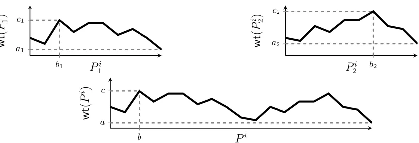
2. IfGhas negative cycles, thenMinCyclereturns a value that is at most a polynomial (inn) factor smaller thanc∗_. U-shaped paths. Following the recent work of [18], we define the important notion of U-shaped paths in a tree-decompositionTree(G). Given a bagBand nodesu, v ∈B, we say that a pathP :u visU-shapedinB, if one of the following conditions hold:

1. Either|P|>1and for all intermediate nodesw∈P, we haveBis an ancestor ofBw,

2. or|P| ≤1andBisBuorBv(i.e.,Bis the root bag of eitheruorv).

that every simple cycleCcan be seen as aU-shaped pathP from the smallest-level node ofCto itself. Consequently, we can determine the valuec∗by only consideringU-shaped paths inTree(G).

Remark 1. Let C = (u1, . . . , uk) be a simple cycle in G, and uj = arg minui∈CLv(ui). Then P = (uj, uj+1, . . . uk, u1, . . . , uj)is aU-shaped path inBuj, andwt(P) =wt(C).

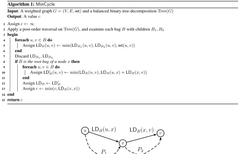
Informal description ofMinCycle.Based on U-shaped paths, the work of [18] presented a method for computing algebraic path properties on tree-decompositions with constant width, where the weights of the edges come from a general semiring. Note that integer-valued weights are a special case of the tropical semiring. Our algorithmMinCycle is similar to the algorithmPreprocessfrom [18]. It consists of a depth-first traversal ofTree(G), and for each examined bagBcomputes alocal distancemapLDB:B×B→Z∪ {∞}such that for eachu, v∈B, we have (i)LDB(u, v) =

wt(P)for some pathP : u v, and (ii)LDB ≤minPwt(P), whereP are taken to be simple u vpaths (or

simple cycles) that areU-shaped inB. This is achieved by traversingTree(G)in post-order, and for each root bagBx

of a nodex, we updateLDBx(u, v)withLDBx(u, x) +LDBx(x, v)(i.e., we do path-shortening from nodeuto node

v, by considering paths that go throughx). See Figure 1 for an illustration.

In the end,MinCyclereturnsminxLDBx(x, x), i.e., the weight of the smallest-weightU-shaped (not necessarily

sim-ple) cycle it has discovered. Algorithm 1 givesMinCyclein pseudocode. For brevity, in line 5 we consider that if {u, v} 6∈Eor{u, v} 6⊆Bifor some childBiofB, thenLDBi(u, v) =∞.

Algorithm 1:MinCycle

Input: A weighted graphG= (V, E,wt)and a balanced binary tree-decompositionTree(G) Output: A valuec

1 Assignc← ∞

2 Apply a post-order traversal onTree(G), and examine each bagBwith childrenB1, B2 3 begin

4 foreachu, v∈Bdo

5 AssignLDB(u, v)←min(LDB1(u, v),LDB2(u, v),wt(u, v))

6 end

7 DiscardLDB1,LDB2

8 ifBis the root bag of a nodexthen

9 foreachu, v∈Bdo

10 AssignLD0_B(u, v)←min(LDB(u, v),LDB(u, x) +LDB(x, v))

11 end

12 AssignLDB ←LD0B

13 Assignc←min(c,LDB(x, x))

14 end

15 returnc

u

x

v

P

P

LD

(

u, x

)

LD

(

x, v

)

Fig. 1: Path shortening in line 10 ofMinCycle. WhenBxis examined,LDBx(u, v)is updated with the weight of the

U-shaped pathP =P1◦P2. The pathsP1andP2areU-shaped paths in the children bagsB1andB2, and we have

In essence,MinCycleperforms repeated summarizations of paths inG. The following lemma follows easily from [18, Lemma 2], and states thatLDB(u, v)is upper bounded by the smallest weight of aU-shaped simpleu vpath inB.

Lemma 2 ([18, Lemma 2]).For every examined bagBand nodesu, v∈B, we have

1. LDB(u, v) =wt(P)for some pathP:u v(andLDB(u, v) =∞if no suchP exists),

2. LDB(u, v)≤minP:u vwt(P)wherePranges overU-shaped simple paths and simple cycles inB.

At the end of the computation, the returned valuecis the weight of a (generally non-simple) cycleC, captured as a U-shaped path on its smallest-level node. The cycleCcan be recovered by tracing backwards the updates of line 10 performed by the algorithm, starting from the nodexthat performed the last update in line 13. Hence, ifCtraversesk distinct edges, we can write

c=wt(C) =

k

X

i=1

ki·wt(ei) (1)

where eacheiis a distinct edge, andkiis the number of times it appears inC.

Lemma 3. Lethbe the height ofTree(G). For everykiin Eq.(1), we haveki≤2h.

Proof. Note that the edgeei = (ui, vi)is first considered byMinCyclein the root bagBiof nodexi, wherexi =

arg maxyi∈{ui,vi}Lv(yi) (line 10). AsMinCycle backtracks from Bi to the root of Tree(G), the edge ei can be

traversed at most twice as many times in each step (because of line 10, once for each term of the sumLDB(u, x) +

LDB(x, v)). Hence, this doubling will occur at mosthtimes, andki≤2h. ut

Lemma 4. Let cbe the value returned byMinCycle,hbe the height ofTree(G), andc∗ = minCwt(C)over all

simple cyclesCinG. The following assertions hold:

1. IfGhas no negative cycles, thenc=c∗. 2. IfGhas a negative cycle, then

(a) c≤c∗.

(b) |c|=O |c∗_{| ·n·2}h .

Proof. By Remark 1, we have thatc∗=wt(P)for aU-shaped pathP :x x. By Lemma 2, afterMinCycleexamines Bx, it will bec≤LDBx(x, x)≤c

∗_{, with the equalities holding if there are no negative cycles inG(by the definition} ofc∗, as thenLDBx(x, x)is witnessed by a simple cycle). By line 10,ccan only decrease afterwards, and again by the

definition ofc∗this can only happen if there are negative cycles inG. This proves items 1 and 2a, and the remaining of the proof focuses on showing that|c|=O |c∗_{| ·n·2}h

.

By rearranging the sum of Eq. (1), we can decompose the obtained cycleCinto a set ofk0+_{non-negative cyclesC}+

i ,

and a set ofk0−negative cyclesC_i−, and each cycleC_i+ andC_i−appears with multiplicityk+_i andk−_i respectively. Then we have

|c|=|wt(C)|=

k0+

X

i=1

k_i+·wt(C_i+) +

k0−

X

i=1

k−_i ·wt(C_i−) ≤ k0− X i=1

k−_i ·wt(C_i−) ≤ k− X i=1

k_i−· |wt(C_i−)| ≤ |c∗| ·

k0−

X

i=1

k_i−≤ |c∗| ·

k

X

i=1

k−_i =O |c∗| ·n·2h

(2)

The first inequality follows fromc <0, the third inequality holds by the definition ofc∗, and the last inequality holds sincek0−≤k. Finally, we havePk

i=1k

−

i =O n·2 h

Next we discuss the time and space complexity ofMinCycle.

Lemma 5. Lethbe the height ofTree(G).MinCycleaccesses each bag ofTree(G)a constant number of times, and usesO(h)additional space.

Proof. MinCycle accesses each bag a constant number of times, as it performs a post-order traversal onTree(G)

(line 2). Because it computes the local distances in a postorder manner, the number of local distance maps LDB

it remembers is bounded by the heighthof Tree(G). SinceTree(G)has constant width,LDB requires a constant

number of words for storing a constant number of nodes and weights in eachB. Hence the total space usage isO(h),

and the result follows. ut

The following theorem summarizes the results of this section.

Theorem 2. LetG = (V, E,wt)be a weighted graph ofnnodes with constant treewidth, and a balanced, binary tree-decompositionTree(G)ofGbe given. Letc∗, be the smallest weight of a simple cycle inG. AlgorithmMinCycle

usesO(n)time andO(logn)additional space, and returns a valuecsuch that:

1. IfGhas no negative cycles, thenc=c∗. 2. IfGhas a negative cycle, then

(a) c≤c∗.

(b) |c|=|c∗_{| ·n}O(1)_.

4

The Minimum Ratio and Mean Cycle Problems

In the current section we present algorithms for solving the minimum ratio and mean cycle problems for weighted graphsG= (V, E,wt,wt0_{)of constant treewidth.}

Remark 2. IfGis not strongly connected, we can compute its maximal strongly connected components (SCCs) in linear time [?], and use the algorithms of this section to compute the minimum cycle ratioν_i∗in every componentGi.

Afterwards, we assign the ratio valuesν∗_{(u)for all nodesuas follows. First, mark every SCCG}

iwithM(Gi) =νi∗.

Then, for every bottom SCCGi, (i) for everyuinGiassignν∗(u) =M(Gi), (ii) for every neighbor SCCGjofGi,

markGj withM(Gj) = min(M(Gj), M(Gi)), (iii) removeGiand repeat. Since these operations require linear time

in total, they do not impact the time complexity. Therefore, we consider graphsGthat are strongly connected, and we will speak about the minimum ratioν∗and meanµ∗values ofG.

In light of Remark 2, we consider graphs that are strongly connected, and hence it follows thatν∗(u)is the same for every nodeu, and thus we will speak about the minimum ratioν∗and meanµ∗values ofG.

Claim 1. Let ν∗ be the ratio value of G. Thenν∗ ≥ ν iff for every cycle C of Gwe havewtν(C) ≥ 0, where

wtν(e) =wt(e)−wt0(e)·νfor each edgee∈E.

Proof. Indeed, for any cycleCwe havewt(C)≥ν∗_{≥ν. Then}

wt(C)≥ν ⇐⇒ wt(C)−ν≥0 ⇐⇒ wt(C)−ν·wt 0_(C) wt0(C) ≥0

⇐⇒wt(C)−ν·wt0(C)≥0 ⇐⇒ X

e∈C

(wt(e)−wt0(e)·ν)≥0 ⇐⇒ wtν(C)≥0

Hence, given a tree-decompositionTree(G), for any guessν of the ratio valueν∗, we can evaluate whetherν∗ ≥ν by constructing the weight functionwtν =wt−νand executing algorithmMinCycleon inputGν = (V, E,wtν). By

Item 2a of Theorem 2 and Claim 1 we have that the returned valuecofMinCycleisc ≥ 0iffwtν(C) ≥ 0for all

cyclesC, iffν∗≥ν(and in factc= 0iffν∗=ν).

Lemma 6. Let G = (V, E,wt,wt0) be a weighted graph of nnodes with constant treewidth and minimum ratio valueν∗. LetTree(G)be a given balanced, binary tree-decomposition ofGof constant width. For any rationalν, the decision problem of whetherν∗≥ν(orν∗=ν) can be solved inO(n)time andO(logn)extra space.

Proof. By Claim 1, we can test whether ν∗ ≥ ν by testing whetherGν = (V, E,wtν)has a negative cycle. By

Theorem 2, a negative cycle inGνcan be detected inO(n)time and usingO(logn)space. ut

4.1 Exact solution

We now describe the method for determining the valueν∗ ofGexactly. This is done by making various guessesν such thatν∗ ≥νand testing for negative cycles in the graphGν = (V, E,wtν). We first determine whetherν∗= 0,

using Lemma 6. In the remaining of this section we assume thatν∗6= 0.

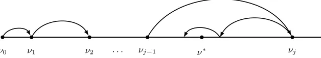
Solution overview.Consider thatν∗ > 0. First, we either find thatν∗ ∈ (0,1)(hencebν∗_{c = 0), or perform an}

exponential searchof O(logν∗)iterations to determine j ∈ N+ such that ν∗ ∈ [2j−1,2j]. In the latter case, we

perform a binary search ofO(logν∗)iterations in the interval[2j−1_,2j_{]to determinebν}∗_{c(see Figure 2). Then, we} can writeν∗ = bν∗_{c+x, wherex < 1 is an irreducible fraction} a0

b. It has been shown [42] that such xcan be

determined by evaluatingO(logb)inequalities of the formx≥ν. The case forν∗<0is handled similarly.

Lemma 7. Letν∗6= 0be the ratio value ofG. The valuebν∗_{ccan be obtained by evaluatingO(log|ν}∗_{|)inequalities}

of the formν∗≥ν.

Proof. First determine whetherν∗ > 0, and assume w.l.o.g. that this is the case (the process is similar ifν∗ < 0). Perform an exponential search on the interval(0,2· bν∗_{c)by a sequence of evaluations of the inequalityν}∗_≥ν

i= 2i.

Afterlogbν∗_{c+ 1 steps we either have bν}∗_{c ∈ (0,1), or have determined a j > 0 such that ν}∗ _{∈ [ν}

j−1, νj].

Then, perform a binary search in the interval[νj−1, νj], until the running interval[`, r]has length at most1. Since

νj−νj−1=νj−1≤ν∗, this will happen after at mostlogdν∗esteps. Then eitherbν∗c=b`corbν∗c=brc, which

can be determined by evaluating the inequalityν∗≥ brc. A similar process can be carried out whenν∗<0. Figure 2

shows an illustration of the search. ut

ν0 ν1 ν2 . . . νj−1 _ν∗ νj

Fig. 2: Exponential search followed by a binary search to determinebν∗_c

LetTmax = maxewt0(e)be the largest weight of an edge wrtwt0. Sinceν∗ is a number with denominator at most

(n−1)·Tmax, it can be determined exactly by carrying the binary search of Lemma 7 until the length of the running

interval becomes at most _((n−1)1_·T

Lemma 8. Letν∗ 6= 0be the ratio value ofG, such thatν∗is the irreducible fractiona_b ∈(−1,1). Thenν∗can be determined by evaluatingO(logb)inequalities of the formν∗≥ν.

Proof. Consider thatν∗ >0(the proof is similar whenν∗ <0). It is shown in [42] that a rational with denominator at mostbcan be determined by evaluatingO(logb)inequalities of the formν∗≥ν. We remark thatbis not required to be known, although the work of [42] assumes that a bound on the denominator ofν∗is known in advance. ut

Theorem 3. LetG= (V, E,wt,wt0)be a weighted graph ofnnodes with constant treewidth, andλ= maxu|au·bu|

such thatν∗(u)is the irreducible fractionau

bu. LetT(G)andS(G)denote the required time and space for constructing

a balanced binary tree-decompositionTree(G)ofGwith constant width. The minimum ratio cycle problem forGcan be computed in

1. O(T(G) +n·log(λ))time andO(S(G) +n)space; and 2. O(S(G) + logn)space.

Proof. In view of Remark 2 the graphGis strongly connected and has a minimum ratio valueν∗. Letν∗=bν∗_c+a0 b

with|a0

b| < 1. By Lemma 7,bν

∗_{ccan be determined by evaluatingO(log|ν}∗_{|) = O(log|a|)inequalities of the} formν∗ ≥ν, and by Lemma 8, a_b0 can be determined by evaluatingO(b)such inequalities. A balanced binary tree-decompositionTree(G)can be constructed once inT(G)time andS(G)space, and stored inO(n)space.Tree(G)

is also a tree-decomposition of everyGνrequired by Claim 1. By Theorem 2 a negative cycle inGν can be detected

inO(n)time and usingO(logn)space. This concludes Item 1. Item 2 is obtained by the same process, but with re-computingTree(G)every timeMinCycletraverses from a bag to a neighbor (thus not storingTree(G)explicitly). u t

Using Theorem 1 we obtain from Theorem 3 the following corollary.

Corollary 1. LetG= (V, E,wt,wt0)be a weighted graph ofnnodes with constant treewidth, andλ= maxu|au·bu|

such thatν∗(u)is the irreducible fraction au

bu. The minimum ratio value problem forGcan be computed in

1. O(n·log(λ))time andO(n)space; and 2. O(logn)space.

By settingwt0(e) = 1for eache∈Ein Corollary 1 we obtain the following corollary for the minimum mean cycle.

Corollary 2. LetG= (V, E,wt)be a weighted graph ofnnodes with constant treewidth, andλ = maxu|µ∗(u)|.

The minimum mean value problem forGcan be computed in

1. O(n·log(λ))time andO(n)space; and 2. O(logn)space.

4.2 Approximating the minimum mean cycle

We now focus on the minimum mean cycle problem, and present algorithms for-approximating the mean valueµ∗ ofGfor any0< <1inO(n·log(n/))time, i.e., independent ofµ∗.

Approximate solution in the absence of negative cycles.We first consider graphsGthat do not have negative cycles. LetCbe a minimum mean value cycle, andC0a minimum weight simple cycle inG, and note thatµ∗∈[0,wt(C0)]. Additionally, we have

wt(C0)≤wt(C) =⇒ wt(C0)≤ n

|C| ·wt(C) =⇒ wt(C

Consider a binary search in the interval[0,wt(C0)], which in stepiapproximatesµ∗ by the right endpointµi of its

current interval. The error is bounded by the length of the interval, henceµi−µ∗≤wt(C0)·2−i≤(n−1)·µ∗·2−i.

To approximate within a factorwe require

2−i·(n−1)≤ =⇒ i≥log(n) + log(1/) (3)

steps.

Remark 3. Note that for the minimum ratio value we havewt(C0)≤W0·n·ν∗, whereW0 = maxe∈Ewt0(e). For

-approximatingν∗we would needi≥log(n·W0/)steps.

Approximate solution in the presence of negative cycles.We now turn our attention to-approximatingµ∗ in the presence of negative cycles inG. Note that uniformly increasing the weight of each edge so that no negative edges exist does not suffice, as the error can be of order· |W−_{|rather than·µ}∗_{, whereW}−_{is the minimum edge weight.} Instead, letc be the value returned byMinCycleon inputG. Item 2a of Theorem 2 guarantees that for the weight functionwt−|c|(e) = wt(e) +|c|, the graphG−|c| = (V, E,wt−|c|)has no negative cycles (although it might still have negative edges). The following lemma states thatµ∗can be-approximated by0-approximating the valueµ0∗of G−|c|, for some0polynomially (inn) smaller than.

Lemma 9. Letµ∗andµ0∗be the value ofGandG−|c|respectively, andsome desired approximation factor ofµ∗,

with0< <1. There exists an0 =/nO(1)_{such that ifµ}0_{is an}0_{-approximation ofµ}0∗_inG

−|c|, thenµ=µ0− |c|

is an-approximation ofµ∗inG.

Proof. By construction, we haveµ0∗_=µ∗_{+|c|, wherecdefined above is the value returned byMinCycleonG. Let} c∗be the weight of a minimum-weight simple cycle inG. By Theorem 2 Item 2b, we have that|c|=|c∗| ·nO(1)_{. Note}

that|c∗_{| ≤(n−1)· |µ}∗_{|, henceµ}0∗_=µ∗_+|c∗_{| ·n}O(1)_{≤ |µ}∗_{| ·αforα=n}O(1)_{. Let}0_{=/α. By}0_{-approximating} µ0∗byµ0we have

|µ0−µ0∗| ≤0· |µ0∗| =⇒ |(µ0− |c|)−(µ0∗− |c|)| ≤0· |µ0∗| =⇒ |µ−µ∗| ≤0· |µ∗| ·α≤· |µ∗|

The desired result follows. ut

Theorem 4. LetG = (V, E,wt)be a weighted graph ofnnodes with constant treewidth. For any0 < < 1, the minimum mean value problem can be-approximated inO(n·log(n/))time andO(n)space.

Proof. In view of Remark 2 the graphGis strongly connected and has a minimum mean valueµ∗. First, we construct a balanced binary tree-decompositionTree(G)ofGinO(n·logn)time andO(n)space Theorem 1. Letc be the value returned byMinCycleon the input graphG. Ifc ≥0, by Lemma 4 we haveµ∗ _{≥0, and by Eq. (3)µ}∗_{can be} -approximated inO(log(n/))steps. Ifc <0, we construct the graphG_−|c|= (V, E,wt−|c|). By Lemma 9,µ∗can be-approximated by0approximating the mean valueµ0∗ofG_−|c|, where0 = nO(1). By construction,G−|c|does not contain negative cycles, thusµ0∗ ≥0, and by Eq. (3)µ0∗can be approximated inO(log(n/0)) =O(log(n/))

steps. By Lemma 5, each step requiresO(n)time. The statement follows. ut

5

The Minimum Initial Credit Problem

(ii) an O(n2 ·m)for the value problem, improving the previously best upper bounds. Afterwards we adapt our approach on graphs of constant treewidth to obtain anO(n·logn)algorithm for the value problem.

Non-positive minimum initial credit.For technical convenience we focus on a variant of the minimum initial credit problem, where energies are non-positive, and the goal is to keep partial sums of path prefixes non-positive. Formally, given a weighted graphG = (V, E,wt), the non-positive minimum initial credit value problem asks to determine for each node u ∈ V the largest energy value E(u) ∈ _Z≤0∪ {−∞}with the following property: there exists an

infinite pathP = (u1, u2. . .)withu = u1, such that for every finite prefixP ofP we haveE(u) +wt(P) ≤ 0.

Conventionally, we letE(u) =−∞if no finite such value exists. The associated decision problem asks given a node uand an initial creditc ∈Z≤0whetherE(u)≥c. Hence, here minimality is wrt the absolute value of the energy. A

solution to the standard minimum initial credit problem can be obtained by inverting the sign of each edge weight and solving the non-positive minimum initial credit problem in the resulting graph.

We start with some definitions and claims that will give the intuition for the algorithms to follow. First, we define the minimum initial credit of a pair of nodesu, v, which is the energy to reachvfromu(i.e., the energy is wrt a finite path).

Finite minimum initial credit.For nodesu, v∈V, we denote withEv(u)∈Z≤0∪ {−∞}the largest value with the

following property: there exists a pathP :u vsuch that for every prefixP0 ofP we haveEv(u) +wt(P0)≤0.

Note that for every pair of nodesu, v∈V, we haveE(u)≥Ev(u) +E(v). Conventionally, we letEv(u) =−∞if no

such value exists (i.e., there is no pathu v).

Remark 4. For anyu∈V, letP :u vbe a witness path forEv(u)>−∞. Then

Ev(u) +wt(P)≤0 =⇒ Ev(u)≤ −wt(P)≤ −d(u, v)

i.e., the energy to reachvfromuis upper bounded by minus the distance fromutov.

Highest-energy nodes.Given a (possibly infinite) pathP withwt(P)<∞, we say that a nodex∈P is a highest-energy node ofP if there exists ahighest-energy prefix P1 of P ending inxsuch that for any prefix P2 of P we

havewt(P1)≥wt(P2). Note that since the weights are integers, for every pair of pathsP10,P20, it is either|wt(P10)−

wt(P₂0)|= 0or|wt(P₁0)−wt(P₂0)| ≥1. Therefore the set{wt(Pi)}iof weights of prefixes ofPhas a maximum, and

thus a highest-energy node always exists whenwt(P)<∞. The following properties are easy to verify:

1. Ifxis a highest-energy node in a pathP :u v, thenEv(x) = 0.

2. Ifxis a highest-energy node in an infinite pathP, thenE(x) = 0.

The following claim states that the energyE(u)of a nodeuis the maximum energyEv(u)to reach a0-energy nodev.

Claim 2. For everyu∈V, we haveE(u) = maxv:E(v)=0Ev(u).

Proof. The directionE(u)≥maxv:E(v)=0Ev(u)is straightforward. For the other direction, consider thatE(u)>−∞

(trivially,−∞ ≤maxv:E(v)=0Ev(u)) and letP be a witness path forE(u). SinceE(u)>−∞, we havewt(P)<∞,

andPhas some highest-energy nodex, thusE(x) = 0. Sincexis on the witnessPofE(u), we haveE(u)≤Ex(u)≤

maxv:E(v)=0Ev(u). The result follows. ut

5.1 The decision problem for general graphs

Here we address the decision problem, namely, given some nodeu ∈ V and an initial creditc ∈ Z≤0, determine

Claim 3. For everyu∈V andc∈Z≤0, we have thatE(u)≥ciff there exists a simple cycleCsuch that (i)wt(C)≤

0and (ii) for everyv∈Cwe have thatEv(u)≥c, which is witnessed by a pathPv:u vwith|Pv|< n.

Proof. For the one direction, ifwt(C)≤0we havewt(Cω)<∞, thusCcontains a0-energy nodew. By Claim 2, E(u) = maxv:E(v)=0Ev(u)≥Ew(u)≥c. For the other direction, letPbe a witness path forE(u), and we can assume

w.l.o.g. thatP does not contain positive cycles. Then for every prefixPv:u vofPwe haveE(u) +wt(Pv)≤0,

thusEv(u)≥E(u)≥c, and then-th such prefix contains a non-positive cycleC. The result follows. ut

AlgorithmDecisionEnergy.Claim 3 suggests a way to decide whetherE(u)≥c. First, we start with energycfrom u, and perform a sequence ofn−1relaxation steps, similar to the Bellman-Ford algorithm, to discover the setVc u

of nodes that can be reached fromuwith initial creditcby a path of length at mostn−1. Afterwards, we perform a Bellman-Ford computation on the subgraphG Vc

u induced by the setVuc. By Claim 3, we have thatE(u) ≥ c

iffG Vc

u contains a non-positive cycle. Algorithm 2 (DecisionEnergy) gives a formal description. Theforloop in

lines 6-12 is similar to the procedure ROUND from the algorithm of [9].

Detecting non-positive cycles.It is known that the Bellman-Ford algorithm can detect negative cycles. To detect non-positive cycles in a graphGwithnnodes and weight functionwt, we execute Bellman-Ford onGwith a slightly modified weight functionwt0 for whichwt0(e) =wt(e)− 1

n. Then for any simple cycleCinGwe havewt(C)≤0

iffwt0(C)<0. Indeed,

wt0(C)<0 ⇐⇒ X

e∈C

wt(e)−X

e∈C

1

n <0 ⇐⇒ wt(C)< |C|

n ⇐⇒ wt(C)≤0

since|C| ≤nandwt(C)∈Z.

Algorithm 2:DecisionEnergy

Input: A weighted graphG= (V, E,wt), a nodeu∈V, an initial energyc∈Z≤0

Output:TrueiffE(u)≥c

// Initialization

1 foreachv∈V do 2 AssignD(s)← ∞ 3 end

4 AssignD(u)←c 5 AssignVc

u← {u}

// n−1 relaxation steps to discover Vuc

6 fori←1ton−1do 7 foreach(v, w)∈Edo

8 ifD(w)≥D(v) +wt(v, w)andD(v) +wt(v, w)≤0then

9 AssignD(w)←D(v) +wt(v, w) 10 AssignV_uc←V_uc∪ {w}

11 end

12 end

13 Execute Bellman-Ford onGVc u

14 returnTrueiff a non-positive cycle is discovered

The correctness ofDecisionEnergyfollows directly from Claim 3. The time complexity isO(n·m)time spent in the

forloop of lines 6-12, plusO(n·m)time for the Bellman-Ford. We thus obtain the following theorem.

Theorem 5. LetG = (V, E,wt)be a weighted graph ofnnodes andmedges. Letu ∈ V be an initial node, and

c ∈ Z≤0be an initial credit. The decision problem of whetherE(u)≥ccan be solved inO(n·m)time andO(n)

5.2 The value problem for general graphs

We now turn our attention to the value version of the minimum initial credit problem, where the task is to determine E(u)for every nodeu. The following claim establishes that if for all energies to reach some nodevwe haveEv(w)<0,

thenEv(u) =−d(u, v), i.e., the energy to reachvfrom every nodeuis minus the distance fromutov.

Claim 4. If for allw∈V \ {v}we haveEv(w)<0, then for eachu∈V \ {v}we haveEv(u) =−d(u, v).

Proof. LetP :u vbe a witness path to the distance, i.e.,wt(P) =d(u, v) <∞(ifd(u, v) = ∞the statement is trivially true). Since every highest-energy nodexofP hasEv(x) = 0, we have thatx=v. Hence,P is a

highest-energy prefix of itself, and for each prefixP0 ofP we have−wt(P) +wt(P0)≤ 0and thusEv(u) ≥ −wt(P) =

−d(u, v). By Remark 4, it isEv(u)≤ −d(u, v). The result follows. ut

AnO(n2_{·m)time solution to the value problem.Claim 4 together with Theorem 5 lead to anO(n}2_{·m)method for}

solving the minimum initial credit value problem. First, we compute the setX ={v ∈V :E(v) = 0}inO(n2·m)

time, by testing whetherE(u) ≥ 0 for each nodeu. Afterwards, we contract the set X to a new node z, and by Claim 2 for every remaining nodeuwe haveE(u) = maxv∈XEv(u) = Ez(u). Sinceu 6∈ X, the energy ofuis

strictly negative, and thusEz(u)<0. Finally, by Claim 4, we haveEz(u) =−d(u, z). Hence it suffices to compute

the distance of each nodeutoz, which can be obtained inO(n·m)time.

In the remaining of this subsection we provide a refined solution ofO(k·n·m)time, wherek=|X|+ 1is the number of0-energy nodes (plus one). Hence this solution is faster in graphs wherek =o(n). This is achieved by algorithm ZeroEnergyNodesfor computing the setXfaster.

Determining the0-energy nodes.The first step for solving the minimum initial credit problem is determining the set Xof all0-energy nodes ofG. To achieve this, we construct the graphG2= (V2, E2,wt2)with a fresh nodez6∈V as

follows:

1. The node set isV2=V ∪ {z},

2. The edge set isE2=E∪({z} ×V),

3. The weight functionwt2:E2→Zis

wt2(u, v) =

0 ifu=z

wt(u, v)otherwise

Remark 5. Since for every outgoing edge(z, x)ofzwe havewt2(z, x) = 0, ifzis a highest-energy node in a path of

G2, so isx. Hence every non-positive cycle inG2has a highest-energy node other thanz.

Note that for everyu∈V, the energyE(u)is the same inGandG2.

AlgorithmZeroEnergyNodes.Algorithm 3 describesZeroEnergyNodesfor obtaining the set of all0-energy nodes in G2. Informally, the algorithm performs a sequence of modifications on a graphG, initially identical toG2. In each

step, the algorithm executes a Bellman-Ford computation on the current graphGwithzas the source node, as long as a non-positive cycleCis discovered. For every suchC, it determines a highest-energy nodewofC, and modifiesG

by replacing every incoming edge(x, w)with an edge(x, z)of the same weight, and then removingw. See Figure 3 for an illustration.

As0-energy nodes are discovered,ZeroEnergyNodesperforms a sequence of modifications to the graphG. We denote withGk _{the graphG after thek-th node has been added toX (andG}0 _=G

2). We also use the superscript-kin our

graph notation to make it specific toGk_(e.g.dk_{(u, z)andE}k

z(u)denote respectively the distance fromutoz, and the

energy to reachzfromuinGk_{). The following two lemmas establish the correctness ofZeroEnergyNodes.}

Algorithm 3:ZeroEnergyNodes

Input: A weighted graphG2= (V2, E2,wt2)

Output: The set{v∈V2\ {z}:E(v) = 0}

1 Initialize setsV←V2,E ←E2and mapwt ←wt2 2 LetG = (V,E,wt)

3 Initialize setX ← ∅ 4 whileTruedo

5 Execute Bellman-Ford from source nodezinG 6 ifexists non-positive cycleCthen

7 Determine a highest-energy nodew6=zinC

8 AssignX←X∪ {w} 9 foreachedge(x, w)∈Edo

10 if(x, z)6∈Ethen

11 AssignE←E∪ {(x, z)}

12 Assignwt(x, z)←wt2(x, w)

13 else

14 Assignwt(x, z)←min(wt2(x, w),wt(x, z))

15 end

16 end

17 AssignV←V\ {w} 18 else

19 returnX 20 end

21 end

Proof. The proof is by induction on the size ofX. It is trivially true when|X| = 0. For the inductive step, letwbe thek+ 1-th node added inX. By line 7,wis a highest-energy node in a non-positive cycleCofGk_{. We split into two}

cases.

1. Ifz 6∈C, thenCis also a cycle ofG, hencewis a highest-energy node in the infinite pathP =Cω _{ofG, and}

E(w) = 0.

2. Ifz ∈C, letxbe the node beforezinC. By the modifications of lines 11 and 14, it iswtk_{(x, z) =wt}

2(x, w0),

wherew0is a node that has been added toXwhen the algorithm run onGi_{for somei < k. It follows thatwis a}

highest-energy node in a pathP :z w0inG2, and thus a highest-energy node in a suffixP0 :w w0ofP,

whereP0is a path inG. HenceEw0(w) = 0. By the induction hypothesis,w0is a0-energy node, i.e.,E(w0) = 0, thus by Claim 2 we haveE(w)≥Ew0(w) = 0.

The result follows. ut

Lemma 11. For everyw∈V :E(w) = 0we havew∈X.

Proof. Consider anyw∈V :E(w) = 0. For somei∈_N, we say thatGi_{“is aware ofw” if eitherG}i_{has a non-positive}

cycleC:w w, orw∈X when|X| =i. Note that whenZeroEnergyNodesterminates there are no non-positive cycles inG|X|_{. Hence, it suffices to argue that there exists ak∈}

Nsuch that for eachi≥k,Giis aware ofw. We first

argue that there exists akfor whichGk_{is aware ofw.}

LetP be a witness forE(w) = 0, henceP traverses a non-positive cycleC1inG, thusC1exists inG0. Then there

exists a smallestj ∈ _Nsuch that some nodew0 of P is identified as a highest-energy node in a non-positive cycle C2(possiblyC1 = C2), and inserted toX. Ifw =w0, we have thatGj is aware ofw. Otherwise, sinceE(w) = 0

non-positive cycleC:w winGj+1_{throughz. Hence eitherG}j _orGj+1_{is aware ofw, thus there exists ak∈}

N

for whichGk_{is aware ofw.}

Finally, observe that the distancedi(w, z)does not increase in anyGi _{fori ≥kuntilwis inserted toX, hence for}

eachi≥k, the graphGi_{is aware ofw. The desired result follows. ut}

Determining the negative-energy nodes.Having computed the setXof all the0-energy nodes ofG, the second step for solving the minimum initial value credit problem is to determine the energy of every other nodeu∈V\X. Recall the graphG|X|_{= (V}|X|_,E|X|_,wt|X|_{)after the end ofZeroEnergyNodes.}

Lemma 12. For everyu∈V \X we haveE(u) =−d|X|_{(u, z).}

Proof. Consider any nodeu∈V \X=V|X|_{\ {z}. By Claim 4, in the graphGwe haveE(u) = max}

v:E(v)=0Ev(u),

and by the correctness ofZeroEnergyNodesfrom Lemma 10 and Lemma 11 we haveX = {v : E(v) = 0}, thus E(u) = maxv∈XEv(u). It is straightforward to verify that at the end ofZeroEnergyNodes, we havemaxv∈XEv(u) =

E|zX|(u), i.e., the maximum energy to reach the setX inGis the energy to reachzinG|X|. For allv ∈ V|X|\ {z}

it isE|zX|(v)<0, otherwise we would haveE(v) = 0and thusv ∈ X andv 6∈V|X|. Then by Claim 4,E| X|

z (u) =

−d|X|_{(u, z). We conclude thatE(u) =−d}|X|_{(u, z). ut}

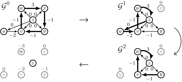
Hence, to compute the energyE(u)of every nodeu∈V \X, it suffices to compute its distance tozinG|X|_{. This} is straightforward by reversing the edges ofG|X|_{and performing a Bellman-Ford computation withzas the source} node. Figure 3 illustrates the algorithms on a small example. We obtain the following theorem.

G

G

G

Fig. 3: Solving the value problem using operations on the graphG. Initially we examineG0, and a non-positive cycle is found (boldface edges) with highest-energy nodex. ThusE(x) = 0, and we proceed withG1_{, to discoverE(u) = 0.}

InG2_{all cycles are positive, and the energy of each remaining node is minus its distance toz.}

Theorem 6. LetG= (V, E,wt)be a weighted graph ofnnodes andmedges, andk=|{v ∈V :E(v) = 0}|+ 1. The minimum initial credit value problem forGcan be solved inO(k·n·m)time andO(n)space.

space in total. The last execution of Bellman-Ford to determine the energy of negative-energy nodes does not affect

the complexity. The result follows. ut

Corollary 3. Let G = (V, E,wt)be a weighted graph ofnnodes andmedges. The minimum initial credit value problem forGcan be solved inO(n2_{·m)time andO(n)space.}

5.3 The value problem for constant-treewidth graphs

We now turn our attention to the minimum initial credit value problem for constant-treewidth graphsG= (V, E,wt). Note that in such graphs m = O(n), thus Theorem 6 gives an O(n3_{)time solution as compared to the existing}

O(n4_{·log(n·W))time solution. This section shows that we can do significantly better, namely reduce the time}

complexity toO(n·logn). This is mainly achieved by algorithmZeroEnergyNodesTWfor computing the setX of

0-energy nodes fast in constant-treewidth graphs.

Extended+ andmin operators.Recall the graph G2 = (V2, E2,wt2) from the last section. GivenTree(G), a

balanced and binary tree-decomposition Tree(G2)of G2 with width increased by 1 can be easily constructed by

(i) insertingzto every bag ofTree(G), and (ii) adding a new root bag that contains onlyz. LetI=Z×V ×Z. For a

mapf :V2×V2→Z, define the mapgf :V2×V2→ Ias

gf(u, v) =

(f(u, v), u,0) iff(u, v)<0orv=z

(f(u, v), v, f(u, v)) otherwise

and for triplets of elementsα1= (a1, b1, c1), α2= (a2, b2, c2)∈ I, define the operations

1. min(α1, α2) =αiwithi= arg minj∈{1,2}aj

2. α1+α2= (a1+a2, b, c), wherec= max(c1, a1+c2)andb=b1ifc=c1elseb=b2.

In words, iffis a weight function, thengf(u, v)selects the weight of the edge(u, v), and its highest-energy node (i.e.,

uiff(u, v)< 0, andvotherwise, except whenv =z), together with the weight to reach that highest energy node node fromu. Recall that algorithmMinCyclefrom Section 3 traverses a tree-decomposition bottom-up, and for each encountered bagB stores a mapLDBsuch thatLDB(u, v)is upper bounded by the weight of the shortestU-shaped

simple pathu v(or simple cycle, ifu=v). Our algorithmZeroEnergyNodesTWfor determining all0-energy nodes is similar, only that nowLDBstores triplets(a, b, c)whereais the weight of aU-shaped pathP,bis a highest-energy

node ofP, andcthe weight of a highest-energy prefix ofP. For two tripletsα1= (a1, b1, c1), α2= (a2, b2, c2)∈ I

corresponding toU-shaped pathsP1 andP2,min(α1, α2)selects the path with the smallest weight, andα1+α2

determines the weight, a highest-energy node, and the weight of a highest-energy prefix of the pathP1◦P2 (see

Figure 4).

AlgorithmZeroEnergyNodesTW.The algorithmZeroEnergyNodesTWfor computing the set of0-energy nodes in constant-treewidth graphs follows the same principle asZeroEnergyNodesfor general graphs. It stores a map of edge weightswt : E2 → Z∪ {∞}, and initiallywt(u, v) = wt2(u, v)for each(u, v) ∈ E2. The algorithm performs a

bottom-up pass, and computes in each bag the local distance mapLDB :B×B → Ithat capturesU-shapedu v

paths, together with their highest-energy nodes. When a non-positive cycleC is found in some bagB, the method KillCycleis called to modify the edges of a highest-energy nodewofC and its incoming neighbors by updating the mapwt. These updates generally affect the distances between the rest of the nodes in the graph, hence some local distance mapsLDB need to be corrected. However, each such edge modification only affects the local distance map

of bags that appear in a path from a bagB0 to some ancestorB00 ofB0. Instead of restarting the computation as in ZeroEnergyNodes, the methodUpdateis called to correct those local distance maps along the pathB0 B00. The following lemma establishes the correctness ofZeroEnergyNodesTW. Similarly as for Lemma 10 and Lemma 11 we denote withGk_{the graph obtained by considering the edges(u, v)for whichwt(u, v)<∞when|X|=k.}

b1

c1

a1

P

wt

(

P

i

)

b2

c2

a2

P

wt

(

P

i

)

b c

a

P

wt

(

P

i

)

Fig. 4: Illustration of theα1+α2 operation, corresponding to concatenating pathsP1andP2. The pathPjidenotes

thei-th prefix ofPj. We haveP =P1◦P2, and the corresponding trippletα= (a, b, c)denotes the weightaofP, its

highest-energy nodeb, and the weightcof a highest-energy prefix.

Algorithm 4:ZeroEnergyNodesTW

Input: A weighted graphG2= (V2, E2,wt2)and a binary tree-decompositionTree(G2)

Output: The set{v∈V2\ {z}:E(v) = 0}

// Initialization

1 AssignX← ∅ 2 foreachu, v∈V2do 3 if(u, v)∈E2then

4 Assignwt(u, v)←wt2(u, v) 5 else

6 Assignwt(u, v)← ∞

7 end

8 end

// Computation

9 Apply a post-order traversal onTree(G), and examine each bagBwith childrenB1, B2 10 begin

11 foreachu, v∈Bdo

12 AssignLDB(u, v)←min(LDB1(u, v),LDB2(u, v), gwt(u, v))

13 end

14 ifBis the root bag of a nodexthen

15 foreachu, v∈Bdo

16 AssignLD0_B(u, v)←min(LDB(u, v),LDB(u, x)+LDB(x, v))

17 end

18 AssignLDB ←LD0B

19 if∃u∈BwithLDB(u, u) = (a, b, c)wherea≤0then

20 AssignX←X∪ {b} 21 ExecuteKillCycleonbandB

Method 5:KillCycle

Input: A0-energy nodewand a bagBofTree(G2)

Output: Updates the local distance functionLDB

1 foreachedge(x, w)∈E2do

2 Assignwt(x, z)←min(wt2(x, w),wt(x, z)) 3 Assignwt(x, w)← ∞

4 Assigny←arg maxu∈{x,w}Lv(u)

5 LetB0be the smallest-level ancestor ofByexamined byZeroEnergyNodesTWso far

6 ExecuteUpdateonByand its ancestorB0

7 end 8 returnLDB

Method 6:Update

Input: A bagB0and an ancestorB00

Output: The local distancesLDBalong the pathB0 B00

1 Traverse the pathB0 B00bottom-up, and examine each bagBwith childrenB1, B2 2 begin

3 foreachu, v∈Bdo

4 AssignLDB(u, v)←min(LDB1(u, v),LDB2(u, v), gwt(u, v))

5 end

6 ifBis the root bag of a nodexthen

7 foreachu, v∈Bdo

8 AssignLD0_B(u, v)←min(LDB(u, v),LDB(u, x)+LDB(x, v))

9 end

10 AssignLDB ←LD0B

11 if∃u∈BwithLDB(u, u) = (a, b, c)wherea≤0then

12 AssignX←X∪ {b} 13 ExecuteKillCycleonbandB

Proof. We only need to argue thatZeroEnergyNodesTWcorrectly computes the non-positive cycles in everyGk_{, as}

then the correctness follows from the correctness Lemma 10 and Lemma 11 ofZeroEnergyNodes. Since by Remark 1 every cycle is aU-shaped path in some bag, it suffices to argue that wheneverZeroEnergyNodesTWexamines a bag B(either directly, or throughUpdate), everyU-shaped simple cycle inBhas been considered by the algorithm. This is true if no calls toKillCycleare made (if block in line 19), as thenZeroEnergyNodesTWis the same asMinCycle, and hence it follows from Lemma 2.

Now consider thatKillCycleis called andB0is the smallest-level bag examined byZeroEnergyNodesTWso far. Letw be the0-energy node,xan incoming neighbor ofw, andy= arg maxu∈{x,w}Lv(u)(as in line 4 ofKillCycle). By the definition ofU-shaped paths, the edge(x, w)appears only in paths that areU-shaped in bags along the pathBy B0.

Hence, after settingwt(x, w) =∞(line 3 ofKillCycle), it suffices to update the local distance maps of these bags. Similarly, after settingwt(x, z)←min(wt2(x, w),wt(x, z))(line 2 ofKillCycle), sinceBzis the root ofTree(G2), it

suffices to update the local distance maps in the bags along the pathBx B0. Eitherx=y, or, by the properties of

tree-decompositions,Bxis an ancestor ofBy. Hence in either caseBx B0is a subpath ofBy B0, and both edge

modifications in lines 2 and 3 are handled correctly by callingUpdateonBy and its ancestorB0. The result follows.

u t

Lemma 14. AlgorithmZeroEnergyNodesTWruns inO(n·logn)time andO(n)space.

Proof. Leth=O(logn)be the height ofTree(G2).

1. The methodUpdateperforms a constant number of operations to each bag in the pathB0 B00whereB00is ancestor ofB0, hence each call toUpdaterequiresO(h)time.

2. The methodKillCycleperforms a constant number of operations locally and one call toUpdatefor each incoming edge ofw. Hence ifwhaskwincoming edges,KillCyclerequiresO(h·kw)time. SinceKillCyclesetswt(x, w) =

∞for all incoming edges ofw, the nodewwill not appear in non-positive cycles thereafter.

3. The algorithmZeroEnergyNodesTWis similar toMinCyclewhich runs inO(n)time and space (Lemma 5). The difference is in the additionalif block in line 19. SinceKillCycleis called when a non-positive cycle is detected, it will be called at most once for each nodeu∈V2\ {z}(from eitherZeroEnergyNodesTWorUpdate). It follows

that the total time ofZeroEnergyNodesTWis

O n+X

u

(h·ku)

!

=O(n+h· |E2|) =O(n·logn)

wherekuis the number of incoming edges of nodeu. SinceKillCyclestores constant size of information in each

bag ofTree(G2), theO(n)space bound follows.

u t

After the setXof0-energy nodes has been computed, it remains to execute one instance of the single-source shortest path problem on the graph G|X| _{(similarly as for our solution on general graphs). It is known that single-source} distances in tree-decompositions of constant treewidth can be computed inO(n)time [23,18]. We thus obtain the following theorem.

Theorem 7. LetG= (V, E,wt)be a weighted graph ofnnodes with constant treewidth. The minimum initial credit value problem forGcan be solved inO(n·logn)time andO(n)space.

6

Experimental Results

6.1 Minimum mean cycle

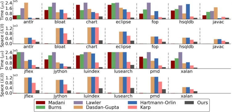
We have implemented our approximation algorithm for the minimum mean cycle problem, and we let the algorithm run for as many iterations until a minimum mean cycle was discovered, instead of terminating afterO(log(n/))iterations required by Theorem 4. We have tested its performance in running time and space against six other minimum mean cycle algorithms from Table 3 in control-flow graphs of programs. The algorithms of Burns and Lawler solve the more general ratio cycle problem, and have been adapted to the mean cycle problem as in [26].

Madani [39] Burns [12] Lawler [38] Dasdan-Gupta [25] Hartmann-Orlin [32] Karp [36]

Time O(n2) O(n3) O(n2·log(n·W)) O(n2) O(n2) O(n2)

Space O(n) O(n) O(n) O(n2) O(n2) O(n2)

Table 3: Asymptotic complexity of compared minimum mean cycle algorithms.

Setup.The algorithms were executed on control-flow graphs of methods of programs from the DaCapo benchmark suit [3], obtained using the Soot framework [46]. For each benchmark we focused on graphs of at least500nodes. This supplied a set of medium sized graphs (between500and1300nodes), in which integer weights were assigned uniformly at random in the range{−103_{, . . . ,10}3_{}. Memory usage was measured with [11].}

Results.Figure 5 shows the average time and space performance of the examined algorithms (bars that exceeded the maximum value in the y-axis have been truncated). Our algorithm has much smaller running time than each other algorithm, in almost all cases. In terms of space, our algorithm significantly outperforms all others, except for the algorithms of Lawler, Burns, and Madani. Both ours and these three algorithms have linear space complexity, but ours also suffers some constant factor overhead from the tree-decomposition (i.e., the same node generally appears in multiple bags). Note that the strong performance of these three algorithms in space is followed by poor performance in running time.

Madani Burns Lawler Dasdan-Gupta Hartmann-Orlin Karp Ours

antlr 55814 61571 165789 284996 21893 7824 18402

bloat 138416 188356 350302 105145 144171 89949 22391 chart 216962 137112 573767 154062 107229 90717 40890 eclipse 216859 242323 667869 172792 148523 107864 23486 fop 83080 147384 406371 59176 121742 31557 19306

hsqldb 131041 153232 208328 86840 228632 40486 19957 javac 58443 110149 122996 179647 14719 34188 20874 jflex 214297 524822 554093 116820 133323 53329 23860

jython 139106 200922 503766 94052 75569 34864 28760 luindex 199650 217980 1240411 274319 228856 92379 22142 lusearch 433211 447280 1180051 263467 333297 101584 55652

pmd 180551 155118 585315 118578 155682 48326 21978 xalan 120897 156111 394458 81103 96873 47996 14493

Table 4: The time performance of Figure 5 (inµs).

6.2 Minimum initial credit

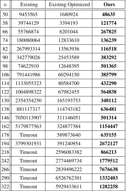
We have implemented our algorithm for the minimum initial credit problem on general graphs and experimentally eval-uated its performance on a subset of benchmark weighted graphs from the DIMACS implementation challenges [1]. Our algorithm was tested against the existing method of [9]. The direct implementation of the algorithm of [9] per-formed poorly, and for this we also implemented an optimized version (using techniques such as caching of intermedi-ate results and early loop termination). Note that we compare algorithms for general graphs, without the low-treewidth restriction.

Setup.For each input graph we first computed its minimum mean valueµ∗using Karp’s algorithm, and then subtracted µ∗from the weight of each edge to ensure that at least one non-positive cycle exists (thus the energies are finite).

Results.Figure 6 depicts the running time of the algorithm of [9] (with and without optimizations) vs our algorithm. A timeout was forced at1010_{µs. Our algorithm is orders of magnitude faster, and scales better than the existing method.}

Madani Burns Lawler Dasdan-Gupta Hartmann-Orlin Karp Ours

antlr 16805 21018 11144 486435 489176 322384 168648 bloat 29723 24500 19458 1245272 1249444 826645 306026 chart 27130 30567 18172 2025448 2029294 1347048 278586 eclipse 24215 26488 16293 965063 968595 640720 254393

fop 16845 17975 11052 576174 578646 382338 169738 hsqldb 16798 19309 11144 486435 489096 322384 168648 javac 14681 17047 9664 372697 375453 247019 144721

jflex 24561 26946 16322 1244495 1248036 826743 251549 jython 22518 23337 14899 1059291 1062570 703581 228207 luindex 39309 40223 25604 3521607 3526792 2342833 399076

lusearch 41488 33350 26991 3387914 3393343 2253403 422679 pmd 32204 24481 21021 1391551 1395786 923975 326137 xalan 16798 17763 11144 486435 489102 322384 168648

Table 5: The space performance of Figure 5 (in KB).

n Existing Existing Optimized Ours

50 9453565 1680924 48635

58 39744129 3394193 121774

66 55766874 6201044 267825

74 180080064 12833610 136239

82 267993314 13563936 116518

90 342779026 25453589 383292

98 74622910 12648395 501365

106 791441986 60294150 385799

114 1133055323 80584700 432290

122 1004898322 67982455 564838

130 2354354250 165193753 348112

138 881117317 114743182 636481

146 7050113907 311146051 501314

162 5179877563 324877384 1154447

178 Timeout 589873640 635155

194 3799301931 391240954 2672127

218 Timeout 2596083382 866213

242 Timeout 2774469734 1779512

266 Timeout 2839496222 7676638

290 Timeout 6526762301 1332403