Some problems in estimation in mixed linear models

Some problems in estimation

in mixed linear models

A thesis submitted for the degree of Doctor of Philosophy

of the Australian National University March 1995

Corrections

Positive line numbers refer to counting from the top of the page, negative line

numbers refer to counting from the bottom of the page.

page 1, line 7: replace "Verbyla and Cullis (1990)" with "Verbyla and Culllis

(1992)".

page 3, line -10: insert at the end of the line. "Methods of checking

identifiability have been investigated by, for example, Rothenberg (1971). He gives

conditions on the identifiability of x which relate principally to properties of the

information matrix."

page 6, line -6: insert at the end of the sentence. "If the true value of the 2

parameter is on the boundary of the parameter space i.e. G()i = 0, then the maximum

likelihood estimate does not have an asymptotic normal distribution, and other

techniques are needed to derive the distribution of the maximum likelihood estimate.

Chernoff (1954) and Moran (1971) show how to proceed in this case."

page 7, lines 5-6: remove the words "projection matrix".

page 18, line 4: insert at the beginning of the line. "A wide range of useful

models fit the conditions (C2.1) - (C2.3), including models with nested random

effects. The methods of proof to follow can be extended to models with crossed

random effects so long as the crossing occurs within independent sub-groups of observations. If such conditions are not met, other arguments will be required. These

seem to require stronger assumptions, such as normality, on the response

distribution."

page 18, line 13: replace "m" with "mj".

page 26, line 8: replace with

" sup sup |{dyi(0)/d0h} - E{dYi(0)/ö0h}| = Op(n)." 0eC(tk) 0: 10 0OI<10 0OI

page 27, line -8: replace "0" with "0".

page 27, line -3: replace "0reml" with "0".

page 54, line -6: insert a new paragraph after this line. "On the other hand,

when using such general estimating equations as (4.3) - (4.4), it is not always easy to

interpret what is being estimated. Naturally, we would like to estimate the parameter

x, but when the data is not necessarily normally distributed, this will not necessarily be

possible. By constructing estimating equations in the manner of (4.3) - (4.4), we estimate whatever quantity makes the mean of (4.3) - (4.4) equal to zero. If \\f is odd

and the distribution of y given X and V is elliptically symmetric, as in Huggins

(1993a, b), then the solution of (4.3) - (4.4) will be x. Otherwise, the solution will

section we have shown how robust estimation methods (3.5) - (3.6) can be derived from the normal likelihood estimating equations (1.6). In this section we return to the

normal likelihood and derive a different representation of the estimating equations. It

is from this representation that Fellner (1986) arrives at his robust estimation method,

which we discuss in the next section."

page 52, line 17: insert at the end of the sentence. "This model is an extension

of the random carriers model studied by Maronna and Yohai (1981)."

page 59, line -9: insert a new paragraph after this line. "For the Mean Value

Theorem to be freely used in this chapter, we will need the function to which it is

applied to be continuous and differentiable at every point: see, for example, Huggins

(1993a, b) for such conditions on \\t functions. While Huber's \\f function is not differentiable at the point k, a suitable approximation to the function that is

differentiable everywhere is \j/(x) = 2 0 (x/k) - 1, where <J> is the standard normal

distribution and K is a constant."

page 63, line 5: replace "9h" with "Th".

page 63, line 8: replace with

" sup sup |{30i(x)/dxh} - E{30i(x)/3xh}| = Op(n)." xeC(tk) x: |x—x0|<|x—x0|

page 78, line 11: replace the first sentence of the section with "We shall assume that (C2.1) - (C2.5) hold i.e. the model is nested. Thus (C5.1) - (C5.5) can be

thought of as identical to (C2.1) - (C2.5)."

page 78, line -12: insert at the end of the sentence. "We also require Aj to be

regular enough to admit a Taylor expansion."

page 85 line 1: insert after "with", "p a twice differentiable function such that"

References

Chernoff, H. (1954). On the distribution of the likelihood ratio. Annals of Mathematical Statistics 25 573-578.

Moran, P.A.P. (1971). Maximum-likelihood estimation in non-standard conditions.

Proceedings of the Cambridge Philosophical Society 70 441-450.

Rothenberg, T.J. (1971). Identification in parametric models. Econometrica 39

577-591.

Verbyla, A.P. and Cullis, B.R. (1992). The analysis of multistratum and spatially

I hereby certify that this thesis does not contain any material previously published or

written by any other person except where due reference is made in the text.

I am indebted to my supervisor, Alan Welsh, for suggesting the problems dealt

with in this thesis, for his guidance in their solution and for stimulating discussions

that have led to many improvements in presentation. I particularly thank my adviser,

Trevor Breusch, for reading draft chapters and providing helpful comments.

I wish to acknowledge the financial support of an ANU Ph.D. scholarship, and

the help and moral support of other Ph.D. students in the Department of Statistics, especially Ian McDermid, Simon Barry and Grace Chan. I also wish to thank Helen

Neave and Erin O'Neill for permission to use data they collected, and Ross

Cunningham for his assistance in initial model building for the data.

I am very grateful to my parents for their encouragement to undertake this course

of study, and I have especially appreciated their regular trips to Australia to visit me.

Finally, I express my deep gratitude to Peter Young for his great love and

This thesis is concerned with the properties of classical estimators of the

parameters in mixed linear models, the development of robust estimators, and the

properties and uses of these estimators. The first chapter contains a review of

estimation in mixed linear models, and a description of four data sets that are used to

illustrate the methods discussed.

In the second chapter, some results about the asymptotic distribution of the

restricted maximum likelihood (REML) estimator of variance components are stated

and proven. Some asymptotic results are also stated and proven for the associated

weighted least squares estimtor of fixed effects. Central limit theorems are obtained

using elementary arguments with only mild conditions on the covariates in the fixed

part of the model and without having to assume that the data are either normally or

spherically symmetrically distributed. It is also shown that the REML and maximum

likelihood estimators of variance components are asymptotically equivalent.

Robust estimators are proposed in the third chapter. These estimators are M -

estimators constructed by applying weight functions to the log-likelihood, the

restricted log-likelihood or the associated estimating equations. These functions

reduce the influence of outlying observations on the parameter estimates. Other

suggestions for robust estimators are also discussed, including Fellner's method. It is shown that Fellner's method is a direct robustification of the REML estimating

equations, as well as being a robust version of Harville's algorithm, which in turn is equivalent to the expectation-maximisation (EM) algorithm of Dempster, Laird and

Rubin.

The robust estimators are then modified in the fourth chapter to define bounded

influence estimators, also known as generalised M or GM estimators in the linear

regression model. Outlying values of both the dependent variable and continuous

independent variables are downweighted, creating estimators which are analogous to the GM estimators of Mallows and Schweppe. Some general results on the asymptotic

properties of bounded influence estimators (of which maximum likelihood, REML and

the robust methods of Chapter 3 are all special cases) are stated and proven. The

method of proof is similar to that employed for the classical estimators in Chapter 2.

Chapter 5 is concerned with the practical problem of selecting covariates in

mixed linear models. In particular, a change of deviance statistic is proposed which

provides an alternative to likelihood ratio test methodology and which can be applied in situations where the components of variance are estimated by REML. The deviance is

specified by the procedure used to estimate the fixed effects and the estimated

covariance matrix is held fixed across different models for the fixed effects. The

distribution of the change of deviance is derived, and a robustification of the change of

Finally, in Chapter 6 a simulation study is undertaken to investigate the

asymptotic properties of the proposed estimators in samples of moderate size. The

empirical influence function of some of the estimators is studied, as is the distribution

of the change of deviance statistic. Issues surrounding bounded influence estimation

Several papers based on the results of this thesis have already been published or

prepared for publication. These are

Richardson, A.M. (1994). Bounded influence estimation in the mixed linear model.

Submitted.

Richardson, A.M. (1995). A comparison of robust likelihood methods for calculating

variance components. Unpublished manuscript.

Richardson, A.M. and Welsh, A.H. (1994a). Asymptotic properties of restricted

maximum likelihood (REML) estimates for hierarchical mixed linear models.

Australian Journal o f Statistics 36 31-43.

Richardson, A.M. and Welsh, A.H. (1994b). Covariate screening in mixed linear

models. Submitted.

Richardson, A.M. and Welsh, A.H. (1995). Robust restricted maximum likelihood in

Contents

Statement of originality i

Acknowledgments ii

Abstract iii

Related publications v

Contents vi

1. Estimation in mixed linear models 1

1.1. Introduction 1

1.2. The mixed linear model 2

1.3. Review of estimation methods 4

1.4. Examples 8

1.4.1. Species richness data 8

1.4.2. Blood data 9

1.4.3. Wheat data 10

1.4.4. Metallic oxide data 11

2. Asymptotic properties of REML estimates 17

2.1. Introduction 17

2.2. Conditions and results 17

2.3. Proofs 22

3. Robust estimation 30

3.1. Introduction 30

3.2. Robust likelihood estimation 32

3.3. Harville's method 35

3.4. Fellner's method 40

3.5. Examples 46

4. Bounded influence estimation 52

4.1. Introduction 52

4.2. The mixed linear model 54

4.3. Choice of weight function 57

4.4. Conditions and results 59

4.5. Proofs 62

4.6. Examples 69

5. Covariate screening 73

vii 5.2. The distribution of the change in deviance 78

5.3. A comparison: log-likelihood ratio and change of deviance 82

5.4. The regression model 84

5.5. The general mixed model 87

5.5.1. Normal deviances 87

5.5.2. General deviances 90

5.6. Examples 93

6. Simulation study 95

6.1. The model 95

6.2. Robust estimation 95

6.3. Covariate screening 98

6.4. Empirical influence functions 103

6.5. Outliers in X 106

6.6. Conclusion 111

References 135

Appendix 1. Data 142

1. Estimation inmixedlinearmodels

l.l. Introduction

Linear models with multiple sources of error, known as mixed linear models, are

used for modelling data from many scientific fields. These include complex sample

surveys (see, for example, Aitkin and Longford (1986) for an application to surveys

of educational achievement), small-area estimation in large-scale surveys (Battese et

al. (1988)), repeated measures experiments (Verbyla and Cullis (1990)), longitudinal

studies or panel data in econometrics (Hsaio (1986)), variety trials in agriculture,

biological experiments and tests of laboratory procedures. This thesis is concerned with the properties of classical estimators of the parameters in mixed linear models, the

modification of these estimators to make them robust, the properties of these new

estimators and their use in covariate screening. Some of the problems addressed are

problems of continuing interest in mixed models which were listed by Engel (1990).

We commence in this chapter with a brief overview of the development of the mixed

linear model and we discuss some classical methods of estimation of its parameters. We also describe four data sets that are used to illustrate the methods developed in this

thesis.

In the second chapter we prove some results about the asymptotic distribution of

restricted maximum likelihood (REML) estimator of variance components. We also prove some related results for the associated weighted least squares estimator of fixed

effects with estimated weights. Central limit theorems are obtained using elementary arguments with only mild conditions on the covariates in the fixed part of the model

and without having to assume that the data are either normally or spherically

symmetrically distributed. We also show that the REML and maximum likelihood

estimates of variance components are asymptotically equivalent.

Chapter 3 concentrates on robustifying maximum likelihood and REML by

constructing M-estimates that reduce the influence of outlying observations on the

parameter estimates. We propose four estimators: Robust ML I and n, and Robust

REML I and II, of which Robust ML I has also been discussed by Huggins (1993a,

b). The Proposal I estimators are constructed by replacing the quadratic function of

the observations in the appropriate log-likelihood by a function with a bounded

derivative. The Proposal II estimators are constructed by replacing the linear function

of the observations in the appropriate estimating equations by a bounded function.

Other suggestions for robust estimators are also discussed, including Fellner's (1986)

method. Fellner's method is a robust version of Harville's (1977) algorithm for

REML estimation of variance components, which is in turn equivalent to the

Fellner's method is also a direct robustification of the REML estimating equations.

We then apply these estimators to two data sets.

The robust estimators proposed in the third chapter are modified in the fourth

chapter to define bounded influence estimators, also known as generalised M or GM

estimators in the linear regression context. Outlying values of continuous independent variables and outlying values of the dependent variable are all downweighted. The

new estimators, which are analogous to the GM estimators of Mallows and Schweppe,

are applied to two data sets. Some general results on the asymptotic properties of

bounded influence estimators (of which maximum likelihood, REML and the robust estimators of Chapter 3 are all special cases) are then stated and proven. The method

of proof is a generalisation of that employed for the classical estimators in Chapter 2.

Next, in Chapter 5, we address the important practical problem of selecting

covariates in mixed linear models when the covariance structure is known from the

data collection process and there are a possibly large number of covariates available.

In particular, a change of deviance statistic is proposed which provides an alternative to likelihood ratio test methodology and which can be applied in situations where the

components of variance are estimated by REML. The key insights are that the

deviance is specified by the procedure used to estimate the fixed effects and that the estimated covariance matrix is held fixed across different models for the fixed effects.

The distribution of the change of deviance statistic is obtained using results from

Chapter 2, without assuming that the model holds. Furthermore, the change of

deviance is straightforward to robustify, in the spirit of Chapters 3 and 4. We show how this is done and derive the distribution of the robust test statistic.

Finally, in Chapter 6 a simulation study is undertaken to investigate the

distribution of the robust and bounded influence estimates in samples of moderate size, using simulated data generated with contamination in none, one or both of the random

effects. We also investigate the distribution of the change of deviance statistic. We

examine the shape of the influence function of some of the robust estimators discussed

in Chapter 3, and discuss the issues associated with bounded influence estimation

when there are outliers in the independent variables.

1.2. The mixed linear model

The general mixed linear model is of the form

c-1

(1.1)

i=I

where y is a n-vector of observations; X and Zi are known n x q and n x pj design

of unobserved random effects, 1 < i < c-1 ; and £ is an n-vector of unobserved

errors. The pi levels of each random effect ßi are assumed to be independent with 2

mean zero and variance a each element of the random error vector e is assumed to

2

be independent with mean zero and variance a oc; and ßi, ßc_i and e are assumed

to be independent. It follows that

2 v*1 2 T

Ey = Xot0 and Var(y) = V = c ocIn + X a 0iZiZi * i=l

It is sometimes useful to put Zc = In and ßc = £, so that (1.1) can be more compactly

written as

y =

c

Xot0 + Zjßj i=l

which leads to

V = I < & £ ■

i=l

We will assume that we have adopted a parameterisation in which all the r = q + c

T T T 2 2

unknown parameters t0 = ( a Q, 0q)t = ( a Q, gq1, ..., a oc)T are identifiable.

The mixed linear model with two variance components is the simplest interesting

mixed model. In this model, we observe yij, where

yij = xToio + ßi + £ij, 1 < i < g; 1 < j < mi,

2 where ßi, ..., ßg are independent random variables with mean zero and variance oq1;

2

£ll> ...» £grrig are independent random variables with mean zero and variance gq2; and

ß l, ..., ßg and E n , — > £gmg are independent. This model is clearly a special case of

(1.1) with c = 2 and pi = g. With y = ( y n , ..., y imi, y2l, y2m2^ •••» ygmg)T,

the model can be written in the form of (1.1) with

A

A

Zi =

img /

where 1 m is a m-vector of ones, and Z2 = In. The n observations y are not independent but the vectors yi = (yn, yimi)T, 1 ^ i ^ g, are independent by virtue of the assumptions on ßi and £y. If the only fixed effect is the mean, the model is also described as fully random and if all the vectors yi are the same length, i.e. there are the same number of observations at each level of ß, or mj = m for all i, then the model is also balanced. Despite its simplicity the two-component model is important in practice because it is applicable to problems where we compare independent clusters of observations. Indeed, three of the data sets we introduce in Section 1.4 fit the two-component model.

1.3. Review ofestimationmethods

If the variance components are known or if estimates of them are available, a weighted least squares estimate of the fixed effects in a mixed model is easily calculated. Variance component estimation is much more troublesome, and the wide variety of ideas put forward to calculate such estimates is an indication of this. The history of these ideas has been dealt with recently and in detail by Searle et al. (1992, ch. 2): here we draw heavily on their work.

The first use of a mixed model was in the work of astronomers Airy (1861) and Chauvenet (1863), who used two-component balanced models. They did not however use the terms "mixed model" or "variance components" and they employed somewhat ad-hoc estimation methods. The first unified approach to estimating the variance components of mixed models consisted of equating various sums of squares of the data to their expected values, and solving for the variance components. These method of moments estimators came to be called analysis of variance (ANOVA) methods, from the term coined by Fisher (1925). In the ensuing two decades a string of papers appeared by many different authors, dealing with ANOVA estimation in either more complex balanced models, or in the simplest (two-component) unbalanced model, that is to say, with an unequal number of observations at each level of ß. The term "variance components" came into common usage during this time as well. Some research into the variance of variance component estimators was also published, for example, by Satterthwaite (1946).

contribute to the error structure of the model. Inferences are made about the entire

population from which the sample of values is drawn, with that inference being based

on the variance of the population. From another point of view, if we are not

interested in the realised values of a variable, we usually treat it as a random effect, otherwise we treat it as a fixed effect. Searle (1992, p.18) provides a flow chart that

highlights the way in which a variable can be fixed or random depending on the type

of inference we wish to make from it.

Returning to the development of estimation methods, Henderson (1953)

proposed three variations on ANOVA estimates for unbalanced models with more than

two random effects. However it became clear that these estimators have several

drawbacks: the form of the estimators is not unique, their distribution is unclear and

there is no guarantee that the estimates will be positive.

However, negative estimates need not be troublesome if we are prepared to

change our assumptions about the structure of the model. In Section 1.2 we assumed

that the observations were built up of fixed effects and random effects with certain

variances. Thus, using the two-component model as an example, the variance matrix

V (which is block diagonal) has diagonal blocks that look like

f 2

1 o + o

oc

2

ol

\

2 2 o + o ,

oc ol

J

2 2

where o > 0 and o , > 0, since both are variances. On the other hand, we could

oc ol

simply assume that the data consisted of a set of observations with a certain mean and

a block diagonal correlation structure. One block of V could then be written

/ 2 \

%cn

y

V

Goc^

J

2 2

where o qc> 0 and g qc + y > 0, to ensure that V remains positive definite. Thus y > —0 qc and y could easily fall in the negative part of its range. The difference between the two correlation structures is subtle, but if it is feasible to use the second structure

for a particular data set, the second structure will accommodate negative ANOVA

estimates.

The disadvantages of ANOVA estimates, along with the advent of high-speed

which united the estimation of fixed effects and variance components. Landmark

papers in this area are those of Hartley and Rao (1967) and Miller (1977). These

authors assumed that the random effects ßi and the errors e in (1.1) are all normally

distributed, and in this case it follows that the observations y are also normally distributed. Thus the log-likelihood is

M V = (—l/2){(y - Xct)Tv-i(y - Xa) + log|V|}.

The n observations y on identifiable linear models involving more than one variance

component are not independent. However we will restrict attention to models where

the random effects are hierarchical or nested. A mathematical definition of nested

effects is given in Section 2.2, but for the present we simply point out that if the

random effects are nested, the vector of observations can always be broken into g independent sub-vectors. Then we may write the log-likelihood as

X(t) = (-1 /2 )X Uyj - XjCiyrv'1 (yj - Xjoc) + log|Vj|}, (1.2) j=l

T T

where y = (yp ..., y g)T and X and V are partitioned conformably. The g mj-vectors

yj are independent so that V is block diagonal with g mj x.m j blocks Vj. The block

diagonal structure of V can also be deduced from the block diagonal structure of each

T T

ZjZ : we will denote the blocks [Z\Z. ]j.

Maximising A^u) for 0 and a is equivalent to solving the following estimating equations, for 0j, 1 < i < c, and a respectively:

(1 /2 )^ (Yj - XjoOTV"1 [Zizir]jV"1(yj - Xjd) - tr[V7' [ZjZ^j] = 0 (1.3)

j=l

The method of maximum likelihood maximises the likelihood over the parameter space,

therefore maximum likelihood estimators of variance components do not suffer from the same problem of negative estimates as ANOVA estimates do. This is important if

one considers the model to be built up of fixed effects and random effects with

associated variances. But maximum likelihood estimators are also known to be badly

biased in small samples; see for example Swallow and Monahan (1984).

To overcome this bias problem, Patterson and Thompson (1971, 1974)

itself. The particular choice of contrasts is unimportant as the log-likelihood always

differs from

r ( 0 ) = (-l/2){yTPy + log|V| + log|XTy-lX|} (1.5)

by at most an additive constant (Harville (1974)). The formula for the projection

matrix P is P = V-1 - V_1X(XTV-1X)-1XTV_1. There are several other ways to

derive (1.5), for instance the conditional approach of Verbyla (1990) and the Bayesian

approach of Harville (1974) and Searle et al. (1992, p.303). We can also regard (1.5)

as a modified profile likelihood from which a has been concentrated out: indeed,

RE ML is sometimes known as marginal maximum likelihood.

The REML estimator of 0oi, 1 < i < c, is obtained by maximising (1.5), and the

estimator satisfies the estimating equations

^i(0) = (-1/2)1 yT0P/39i)y + trtV-lZiZ7; ]

- tr[(XTV-lX)-lXTV-lZiZ7 V-lX]) = 0.

Since Py = V-1(y - Xa(9)), where

<X(0) = ( x T v - 'x r 'x T v - i y ,

'Pj(Ö) = (l/2){(y-X a(9))T V-iZjZ7 V-i(y-Xa(9)) - tr[PZiZ7 ]} = 0. (1.6)

The matrix P is not block diagonal so we cannot write 4^(0) as a sum over

independent groups of observations. Given an estimate 0 of 0O which leads to an estimate V of V, the fixed-effect parameter cxo can be estimated by the weighted least

squares estimator a(0) = (XTV-1X)_1XTV-1y. The weighted least squares estimator

is also the solution for a of

Equation (1.7) is the same as (1.4), except that (1.7) is a function of a alone, whereas (1.4) is a function of both a and 0. Techniques for solving (1.3) and (1.6) are

discussed by Harville (1977).

4^(0) may be more conveniently written as

j=l

Other methods for estimating the parameters of (1.1) have been put forward,

including MINQUE (Minimum Norm Quadratic Unbiased Estimation) and MIVQUE

(Minimum Variance Quadratic Unbiased Estimation). For a clear introduction to these

types of estimation, see Rao and Kleffe (1988). However, Harville (1977) notes that under normality and Euclidean norm, MIVQUE is equivalent to MINQUE. Under

these conditions Searle et al. (1992, sec. 2.4c) note too that MINQUE is also

equivalent to the first iteration of REML. Thus MINQUE and MIVQUE are equivalent

to one-step REML estimation and since this thesis focuses on likelihood-based

methods of estimation, we will not consider MINQUE and MIVQUE further.

1.4. Examples

In this section we describe four data sets from various fields of scientific study

used to illustrate the methods discussed in this thesis: the data sets themselves are

listed in Appendix 1. The structure of the data sets and the kind of inferences required

meant that it was straightforward to decide which were the fixed effects and which

were the random effects for all four data sets.

The first three data sets have two random effects, including random error, while

the last is a more structured data set with four random effects. The fixed effects of the

first two data sets consist of a mixture of dummy variables and continuous covariates.

Such structure is rare in examples in the literature of mathematical statistics, but it is important in the context of bounded influence estimation since bounded influence

methods have no impact on fixed effects that appear in X as dummy variables, e.g. the levels of a categorical variable. The fixed effects of the last two data sets are made up

solely of such categorical variables.

1.4.1. Species richness data

This study, described by Neave (1993), is concerned with the diversity of bird

species in the forests of southeast New South Wales, Australia. A total of 23 domains

were chosen for their different climate and nutrient combinations, and the aspect

(north-facing, south-facing or on a ridge) of 1 hectare sites within each domain was

recorded. Twenty domains had two sites at each aspect and the remaining domains

had one site at each aspect, resulting in a total of 129 sites. The minimum temperature

in the coldest month, and the plant species present at each site were also recorded.

Hybrid multidimensional scaling in four dimensions was applied to the plant species

counts, but only two of the resulting four scores are used here. These scores are

denoted floristicsl and floristics2. The response variable is a simple count of the

A plot of the response against each fixed effect separately is displayed in Figure

1.1, with the observations coded by site number. The fact that the response is a count suggests the use of a log transformation prior to modelling. However there are no

zero counts, and a Q-Q plot of the counts appears approximately normal, so we

proceed with analysis on the raw scale. There appears to be some grouping of the

sites by temperature, but this is simply to do with the way in which the sites were

chosen. There do not appear to be any outlying values in either X or y. A mixed linear model to describe this data is

yij = ji + otk + Yixiij + Y2x 2ij + Y3x 3ij + ßi + £ij,

1 < i < 23, 1 < j < 3 or 6, 1 < k < 3

where yjj is the species richness at the site in the i^ domain; (X is the overall mean;

otk is the fixed effect due to aspect, where k denotes the aspect of the j 1*1 site in the Ith

domain; xnj, X2ij and X3ij are the values of the fixed effects floristicsl, floristics2 and

minimum temperature respectively at the site in the Ith domain, and Yl, Y2 and Y3

are the associated slope parameters; ßi is the random effect due to domain i, assumed

2

to be a random variable with mean zero and variance G ^ , £y is random error, assumed 2

to be a random variable with mean zero and variance a £; and all the variables on the

right-hand side are independent. For identifiability purposes, we set oiN-facing = 0. Naturally, other parameterisations are possible.

This data set contains continuous covariates, so we will use it in Chapter 4 to

illustrate the use of bounded influence methods. We also use it in Chapter 5 to

illustrate a simple application of the change of deviance test.

1.4.2. BLOOD DATA

An experiment was conducted by O'Neill (1993) to investigate the relationship between infectious diseases and nitric oxide (NO) levels in human blood. One or two

blood samples were obtained from 78 individuals in five groups: Australians who were free of disease (17 individuals); Caucasians living in Indonesia who were also free of disease (11); and Indonesian nationals who were free of disease (10), those with dengue fever (19) and those with typhoid (21). In analysing this data and in listing it in Appendix 1, these five groups are treated as two factors each with three levels. The first factor is population, with levels Australian (A), Indonesian Caucasian (IC) and

Indonesian national (IN). The second factor is disease within population, with levels

disease free (C), dengue (D) and typhoid (T). Only five of the nine possible

combinations of these factors were observed.

All diseased individuals had two samples taken, except for one with dengue and

disease-free individuals had only one sample taken, except for one Australian. In total

46 people were sampled once and 32 twice, resulting in 110 observations. The NO

level in each sample was measured by electron spin resonance using a spectrometer.

The output from the spectrometer consists of a spectrum with seven peaks: one for NO and three for each of two types of low spin methaemoglobin, denoted A and B. The

relationship between the height of the three A peaks and the three B peaks meant that

the most suitable variables to include in the model are simply the average heights of

the three A peaks and the three B peaks. There were a number of zero readings

amongst the heights of the NO peak, and the distribution of these heights was skewed.

A transformation was taken to achieve normality, while taking account of the zero

readings: we let yij = log(height of NO peak + 0.1).

A mixed linear model that describes the data is

yij = |l + otk + Tkh + öiaij + §2bij + ßi + £ij,

1 < k < 3, 1 < h < 3, 1 < i < 78, 1 < j < 1 or 2

where yy is the log(height of NO peak + 0.1) of the 1th reading from the Ith

individual. The overall mean is p; otk is the fixed effect due to population group k; ykh

is the fixed effect due to disease h within population group k; aij and by are the

average heights of the A and B peaks respectively and 8i and 8 2 are the associated

slope parameters; ßi is the effect due to individual i, a random variable with mean zero

2

and variance ey is random error, a random variable with mean zero and variance

2

g£; and all the variables on the right-hand side are independent. For identifiability purposes we set cy, the effect due to Australians, equal to zero.

In Figure 1.2 log(NO + 0.1) measurements are plotted against A, B and the five observed combinations of population group and disease. The observations are coded

by individual number. There is one value of A which may turn out to be an outlier in

the independent variables becuase it lies far from the bulk of the values of A. On the

other hand, values of B are more evenly spread through the range of B. There do not

appear to be any outlying values of y, basically because the log transformation has

already been taken.

Because this data set contains continuous covariates, it will be used in Chapter 4

to illustrate the use of bounded influence methods.

1.4.3. WHEAT DATA

This experiment was described by Patterson and Silvey (1980) and re-examined

by Patterson and Nabugoomu (1992). Six varieties of wheat were grown at ten

centres that formed a sample of the main types of growing area for wheat in Scotland,

o f 60 possible variety-centre combinations, only 46 were used. At three centres all

six varieties were grown but at the other seven, only four varieties were grown. A

mixed linear model can therefore be fitted to this data as follows:

yij = p, + Oj + ßi + Sy, 1 < i < 10, 1 < j < 4 or 6

where yy is the yield from the j th variety at the Ith centre; 11 is the overall mean; (Xj is

the fixed effect due to variety j; ßi is the effect due to centre i, a random variable with 2

mean zero and variance £y is random error, a random variable with mean zero and

2

variance G£; and all the variables on the right-hand side are independent.

Patterson and Nabugoomu (1992) also consider a more complex model involving

variety by centre interaction, (aß)y, which is another random effect. Inclusion o f this

effect depends on already having an estimate of the variation within each variety-centre

combination, or on having multiple observations at each variety-centre combination so

that the extra variance component can be estimated.

In Figure 1.3 the yields are plotted against variety, with each observation coded

by centre number. There are no obvious outliers. There does appear to be a definite

ordering of centres, for example, centre 8 produces the highest yield for each variety

grown there, and centre 10 produces the lowest yield. The unbalanced nature of the

data is also clear from the plot, with different centres appearing in the column of yields

for each variety.

This data set will be used to illustrate the robust methods of Chapter 3. We set

the mean, p,, equal to zero so that all the variety effects are identifiable. This makes

comparisons between the estimation o f the six variety effects more straightforward. In

Chapter 5 we use this data again, to test the hypothesis that there is no difference

between the six varieties o f wheat. Then we use a more common identifiability

constraint and set a i , the effect due to Huntsman variety, equal to zero.

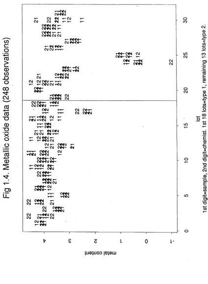
1.4.4. METALLIC OXIDE DATA

Fellner (1986) describes this experiment exploring sources o f variation in the

measurement of the properties of 18 lots of one type of metallic oxide, and 13 lots of

another. Two samples were drawn from each lot and each sample was analysed twice

by two different chemists. Metal content minus 80% by weight was recorded in each

case, and no observations were missed, resulting in a balanced experiment with 248

observations. A mixed linear model for yijkhm» the m^1 measurement of metal content

o f the k^ sample from the lot of the i^ metallic oxide analysed by the 11th chemist,

is as follows:

1 < i < 2, 1 < j < 13 or 18, 1 < k < 2, 1 < h < 2, 1 < m < 2

where fj. is the overall mean; 0Ci is the fixed effect due to type i; ßjj is the effect due to

lot j within type i, a random variable with mean zero and variance (jj ; yijk is the

effect due to sample k within lot j within type i, a random variable with mean zero and 2

variance ^ sample; öijkh is the effect due to chemist h within sample k within lot j within 2

type i, a random variable with mean zero and variance tfchemist; Eijkhm is random 2

error, a random variable with mean zero and variance g£; and all the variables on the

right-hand side are independent. Like Fellner, we set p, = 0 for identifiability

purposes. Although this is a non-standard constraint to apply, it enables us to

compare the estimates of a i and ot2 directly when we use this data to illustrate the robust methods of Chapter 3.

Figure 1.4 displays the metal contents against lot number. The first 18 lots

belong to oxide type 1 and the remainder to oxide type 2. Each observation is plotted

with a code kh, where k is the sample number and h is the chemist number. We see

that for the bulk of the lots, there is little difference in metal content, except for two

F

ig

.

1

.1

.

Sp

ecies

ri

c

h

n

e

s

s

da

ta

(

1

2

9

ob

ser

vat

ions

)

sseuijou SS0UL|OjJ

o c\i

iq

Ö

o

d

OS 03 01. S

ssauipu sseuipu

jc

s

1

flo

ris

tic

s

F

ig

.

1

.

2

.

B

lo

o

d

d

a

ta

(

1

1

0

obse

rvatio

ns)

( l-'O + ON)ul

c o

3

Q.

O

Q_ T3

0)

CD

- Q

E

13

C W_c o

T3

£

CD

</3

JD

O

2 I. 0 V- Z

-(lO + ON)u|

2 1 0 1- 2-

U o + o n)ui

<

a

c

c

o

F

ig

.

1

.3

.

W

h

e

a

t

d

a

ta

(

4

6

ob

ser

vat

ions

)

=5

6 8 Z 9 8

P

(D O O O) .E ■a o o o

. 2 'S

« m > -O E 3 C (0 c g

*

£

O

F

ig

1

.4

.

Me

ta

lli

c

o

x

id

e

d

a

ta

(

2

4

8

obs

er

va

tio

ns

)

T-CMMM CM -r- C W d CM x - CMMM x - x - CM-CM CM CM

X- CMMM- CM CM-CM-x - CM CMM-

CM CM x iT

-CMM- x-CM CMMM xMM T - CM-CM CM CM tt CM CM CM CM CMM x x x -x - x - CMM CM xCM

O N

-c m m

-x-CMMM CM CM-CMM CM

O

CO

■HfM- CMM CMM— C M - CMM ID CM CMMM CM CM O CM

CM C M -x- x€M M CM CMMM x x x - CMM x x x - X-C4M CM X

CMM x x C M x - x x x - CMM

x x C f d

X - X - CM CMM CM CM CM x x

CM CM -x- CM CMMM

X- CM CMM X- x - 1— CMM CM

CM x - CMMM x

-X- CM CMM- CM

t x x CMMM CM

xCMM CMMM -T—

CM CM C M - CMMMM C M - x - CMMM C M - x - x x x - CMM CM CMM— CM CM-x-

CMMM x - xCMM CM « CMM CM C M M M x

-CMMM 'f-T— xMMM CM CM CM CM

CMMM X-

xx-CM CM CM CMMM- CM x-CMMM x-r-CMM CM CM" « « CM CM CM— x - CMM

CM <D Q . cn o _C ’ c aJ

I

1-1U01UOO |E}0UJ

2. Asymptotic properties ofREML estimates

2.1. Intr oduction

In this chapter we address the asymptotic properties of the REML estimator of

0O and the asymptotic properties of the associated weighted least squares estimator of

a 0. We also investigate the relationship between the REML and maximum likelihood

estimators of variance components.

Research into the asymptotic properties of maximum likelihood estimators of T0

commenced with Hartley and Rao (1967) and Miller (1977). The asymptotic

distribution of the REML estimator of 0O was obtained recently by Cressie and Lahiri (1993) using elegant arguments developed by Sweeting (1980). However all these

results require the strong assumption that the observations y are normally distributed

and the question of how these results are affected when y is not normally distributed

has not been discussed. Some results in this direction have been obtained by Huggins

(1993b). His results use martingale arguments but require the assumption that the

independent subvectors yi, 1 < i < g, each have a spherically symmetric distribution. On the other hand, a result for the simple two-component fully random model

where the observations are not necessarily normally distributed was obtained by

Westfall (1987). He assumed that the model is hierarchical, which in practical terms means that y can be partitioned into independent sub-vectors. For more general

hierarchical models, Westfall (1986) explored the properties of the ANOVA estimators of 0O, also for possibly non-normally distributed observations. It is clear that

Westfall's approach provides the best method of obtaining general results without

strong distributional assumptions such as the assumption of normality. Furthermore, it

has the advantage that the proofs require only elementary arguments. We will use this approach here to obtain results for the REML estimators under weaker assumptions on

the fixed effect structure than adopted by Westfall (1986).

We present and discuss the conditions and results in Section 2.2, and give the

proofs in Section 2.3. These proofs will be generalised in Chapter 4 to find the

asymptotic properties of more general estimators.

2.2. CONDITIONS AND RESULTS

Following Westfall (1986), we will assume that the random effects are nested in

the sense that

(C2.1) the n x pj matrices 7,\ are block diagonal with exactly one 1 and pi - 1

(C2.2) pi < pi+i for i < c,

(C2.3) every column in Zi is the sum of some columns in Zi+i for all i < c, and

in forming each sum, no column of Zj+i is used more than once.

Condition (C2.3) ensures that there is no block of ones in Zi+i which extends over

more than a single block in Zi, i < c. For this kind of model, we can partition the

observations y into g independent mj-vectors yj so that the g variables yj - Xjoc are

independent with mean zero and variance Vj. If the data are balanced, mj = m and these sub-vectors are also identically distributed but not otherwise. In the regression

model, m = 1. Westfall (1986) used the hierarchical structure induced by (C2.1) -

(C2.3) structure in his study of ANOVA estimates for non-normal mixed models, but

we do not insist that X also has a hierarchical structure. That is, we weaken his

conditions to allow the fixed effects to contain general covariates.

It is apparent for the two-component model that if we hold g fixed and let m —»

2

°o, we cannot estimate gq1 consistently. However, if we let g —» °o, both variance components can be estimated consistently. For the general model (1.1), we require g

—> oo in such a way as to preserve the nested structure of the random effects in the

model. First, let Li, ..., L5 be a set of constants, not necessarily equal. Then we will require {mj} to be a bounded sequence of positive integers and pi —» °° as g —>

00 such that

(C2.5) if z(i,k) denotes the k1*1 column of Zi, there is a constant L] such that

z(i,k)Tz(i,k) < Li for all n, 1 < k < pi and 1 < i < c-1.

Condition (C2.4) determines the way in which the pi —» 00 and (C2.5) requires that

the number of non-zero entries in the k^ column of Zi is bounded. This means that

as g —> 00 new groups of observations that enter that data set contribute to new

columns of Zi rather than continuously adding rows, which is essential if the block

diagonal structure is to be preserved. Note that min(mj) < g-1n < max(mj) so n and g

are of the same order of magnitude. Moreover, (C2.5) implies that tr[Zj Zi] < piLi.

We also require conditions which enable us to control the asymptotic behaviour

of the estimating equations and their derivatives. These same conditions, along with

the assumptions made about the variance structure of (1.1) will also ensure continuity

so that the Mean Value Theorem can be freely used. Let ||A|| = (trfAAT])1/2 denote (C2.4) pi/ mj —> aj for 1 < i < c-1, where 0 < ai < a2 < ... < ac =

the Euclidean norm of the matrix A. Since |Ax| < ||A|||x|, we have |xTAx| < ||A |||x|2

and ||A B ! < ||A||||B||. We will impose

(C2.6) there is a 5 > 0 and a constant L2 < 00 such that E|yj - XjOol44^ < L2

for all j = 1, 2, ... and i H £ ||Xj||2+* = 0(1), j=l

(C2.7) each component of 0O is positive and finite, 0OC is strictly positive and

finite, and there is a neighbourhood U0 of 0O such that for all j = 1, 2,

..., Vj is nonsingular for all 0 g U0 and || V j 1 || is bounded uniformly in

0 g U0 and j = 1, 2, ...,

(C2.8) letting VQ denote V evaluated at 0O, the matrices

1 ^ T - l

n-1 2j X. V • Xj —> Gaa which is a nonsingular q x q matrix, j=l

( 2 n ) - 'i ; t r [ V ‘ l [ZkZ^]jV“ l [ZiZlT]j] -► [Geelik, 1 < i, k < c, where the j=l

c x c matrix Gee = ([Gee]ik) is positive definite, and

(4n)-i £ {E(yj - X j o j T v i [Z1Z^]JV - 1(yJ-X Ja 0)(yJ-X Ja 0)T x

j=l

Vqi‘ [ZkZ^ljV~1 (yj - XjOo) - tr[V ;] [ Z ^ M ^ ' [ Z kZ ^ ] )

-> [Fee]ik? 1 < i, k < c.

These are mild conditions which will often be satisfied in practice. If x^k denotes the

kth row of Xj, we have for some L3 < °o,

n - 1 i IXjP+S < L3n- l £ ^ |Xjk|2+8 = 0 (l),

j=l j=l k=l

which, on relabelling the covariates, is the regression model condition

n

This condition may be checked for specific sequences of designs, and any sequence suitable for regression modelling will be a suitable fixed part of a mixed model. By virtue of the fact that all the entries of Zj are zero or one, we have ||[ZiZ|']j|| < mj <

L4 uniformly in i and j. This and the bound on HV" 1 || enable us to control

complicated terms in our expansions. For the two component model

/ T

' 1 1

mi mi

T

Ziz! =

v

\

and Z2Z , = In

ig ing

J

V =

( V 1

\

v g y

with Vj = a ^ lmjl^ . + a22Imj.

Furthermore, for the two-component model

V- 1 = - + < I,

so Vj is nonsingular in a neighbourhood U0 of 0O which bounds g2 away from zero,

Mw»—In 2 . 2 2. 1 2 2 1 /2 .. w

IIVj II < g2 (G2 + mjG1) -1a 1mj + G2 mj < L5 < 00,

uniformly in 0 e UQ and j = 1, 2, ... and (C2.7) is satisfied. Thus provided g —> 00

in accordance with (C2.4) - (C2.5) (which it does in the balanced case when mj = m) and the mild conditions (C2.6) and (C2.8) hold, our results below are applicable to this important model. The applicability of the results to more complex models can be checked in a similar way.

In Section 2.3, we will prove the following three results. Theorem 2.1 provides an asymptotic representation and hence the asymptotic distribution of a consistent root of the REML estimating equations. Let 0 (0 ) denote the c-vector with components

which is equivalent to (1.3) with a fixed at a 0.

THEOREM 2.1. Suppose that conditions (C2.1) - (C2.8) hold. Then a solution 0REML to the estimating equations (1.6) which satisfies n 1/ 2|0REML — ö0| = Op( 1) as

n —» °o exists in probability. Moreover,

Note that under normality, Gee =

Fee-We have presented our result on the natural scale. There is some appeal in using

the log scale, because in the one component case Kendall et al. (1983, secs. 37.10 -

37.14) noted that the approach to normality of log s2 is faster than that of s2, a result

which may extend to the case of estimates of multiple variance components. Simple

Taylor series arguments from Theorem 2.1 yield the required asymptotic results for logs, ratios or other parameterisations of interest, say h(0) = (hi(0), ..., hc(0))T. In

that case

n 1/2(0REML - 0O) = n */2G 00O(0o) + op(l),

whence

n 1/ 2(0REML - 9o) N(0, GqqFggG qq).

n ‘/2(h(eREML) - h(60)) = n_1/2H(60)G + op(l)

where

[H(e0)]ik = OhiOVaek)!^.

In particular, if we estimate Gee and Fee by

and [Fee]ik = ( 4 n ) - l £ { ( y j - X ja ) ^ j 1 [ZiZ^]jVj 1(yj - X jä ) ( y j - X j ä ) T V j1 x j=l

[ZkZ^ljV '(yj - Xjöt) - trtVj1 [Z.Z^jJtrtV '[ZkZ^]j]}

respectively, we have the following approximate 100(1 - a)% confidence interval for

l°g(ÖREMLj) ± 0-1(1 - a /2 )0 2 n-l/2[GegFeeG ^ ] ‘/ 2

where O denotes the standard normal distribution function. Back-transforming from the log scale, we obtain

(0REMLiexp[-O-i(l - a/2)6~2 n - l/^ G ^ F e e G '^ ] 1/ 2 ],

eREMLiexp[a>-i(l - a /2 )6 “2 n-i^fO egFeeG “^ ]* /2 ]).

The form of the asymptotic representation in Theorem 2.1 suggests that there is a

close connection between REML and maximum likelihood estimation. That this is

indeed the case is shown in the following corollary.

COROLLARY. Suppose that conditions (C2.1) - (C2.8) hold. Then solutions 0ml

and 0REML to the estimating equations (1.3) and (1.6) respectively which satisfy n 1/ 2(0REML ~ 0ml) = op( l) as n —> °o exist in probability.

This result may be regarded as rather unpalatable, implying that REML has no

advantages over maximum likelihood. However it is important to remember that

REML was devised to have small sample advantages over maximum likelihood estimates, while this result highlights the large sample similarities of REML and maximum likelihood. This corollary does not reduce the usefulness of REML for

estimation in data sets of small to moderate size.

Finally, we show that the weighted least squares estimator of the fixed effects

behaves as expected asymptotically. In fact, it has the same distribution as the

maximum likelihood estimator of the fixed effects and there are no extra terms required

in the variance of the estimator to take account of the fact that the weights are not

known but have been estimated.

THEOREM 2.2. Suppose that conditions (C2.1) - (C2.8) hold. Then a solution

9REML to (1.6) exists in probabihty such that

n 1/2(a(0R£ML) ~ oto) - ? N(0, G "^), as n -> «>.

2.3. PROOFS

The proof of Theorem 2.1 is based on a linear approximation to the estimating

(2.1)

sup n-l/2|vFi(0) - Oi(0o) - EOi(0) + EOi(0o)| = op(l).

le-SolSn-1/ ^

Now, dropping the factor of (1/2) from the estimating equations, we have that

'Fi(e) = (y - Xa(0))TV- i ZiZ^ V->(y - Xa(0))

- tr[V_1ZjZ^] + tr[(XTV -1X )-| XTV~1ZjZ^ V~'X]

OiOo) = (y - XOo)TV 0' Z iZ V 'fy - Xa0) - tr[V;'ZiZ^

EOj(0) = tr[V0V"1 ZjZ^V- 1 ] - trlV-lZiZj]

E<Di(0o) = 0

'Fj(ö) - <t>i(0o) - EOi(0) + E<J>i(0o) = tr[(XTV-lX)-'XTV-lZiZTi V->X]

- 2(a(0) - a 0)XTv-lZjZ^ V~i(y - XOo)

+ (a(0) - (Xo)XTv-iZiZ^ V->X(a(0) - a,,)

+ (y - Xoo^V-iZjZ^ V -'(y - Xcto)

-

z,zV'(y -

-tr[V 0V -lZiZfv-l]

+ tT [ \' Z i Z j ]

after adding and subtracting X a0 in (y - Xa(0))TV_1ZjZy V_1(y - Xa(0)).

To show that the first trace term in (2.2) is op(l), first note that

n~| /2(XTV_lX - XTV“ ' X) = n_ |/2(XT(V_l - V“ ’ )X)

= n-1/2 X XTV-'Z^V-IXfO - 0o)i

i=l

= 0(1).

This controls the behaviour of (X^V-lX)-1 and so

sup n -1/2|tr[(XTV-‘X)-'XTV-1ZiZTi V-'X ]| = op(l).

|e -0 o|<n-1/ 2M

(2.2)

For the next two terms of (2.2) we have that

a(0) - a(0o) = ((XTv-'X)-i - (XTV 'o X)-i)XTVo‘(y - X«o)

+ (XTV-lX)-'XT(V-' - V“1 )(y - Xa0)

and

sup

0 -0 o|<n-1/^M

n-l/2 t x j c v r 1

j=l

< sup X ln_1 i

|e -0 o|^n l / 2M i=i j=l

- \ y ‘)(yj - XjOo)l

x ]'v j' l[Zizjr]jv ;jl(yj - XjOto)| nl/2|(6 - 0o)i|

< M

1

1

xV /K Z ^ V ^ yj -

i=l j=l

+ M

i--'t

-> 0

so

sup n1/2|a(0) - (XqI = Op(l).

|e -0 o|<n-1/ 2M

(2.4)

Similar arguments can be used to show that

sup n-l/2|xTv-lZiZT. V-l(y - XOo)| = Op(l)

|0-0o|<n_1/ 2M

and hence we have

sup n-i/2|2(a(6) - a 0)TXTV-lZ,ZTi V">(y - Xoto)|

|0-0o|<n-1/ 2M

+ sup n - i/2 |( a (e ) - a 0)TxTv-iZiZTi V -> X (a (e )-a 0)|=Op(l).

|0-0o|<n_1/ 2M

Cover the ball {|t| < n-1/ 2M} with cubes C = {C(tk)}, where C(tk) is a cube

containing tk with sides of length n-1/2-l/4cfy[. It follows that N = card(C) =

(X n1/4), |tk| ^ n-1/2M and for t e C(tk), |t - tk| < n-1/2 -l/4 c ^ Then let

Yi(0) = (y - X a 0)T V -lZ jZ ^ V -l(y - XOo), 1 < i < c.

The last four terms of (2.2) are Yi(0) - Yi(0o) - Eyj(0) + Eyj(0o). We first show that

this difference is op(l) not for sup 0: {|0 - 0O| < n-1/2M}, but for the sum over C of

fixed tk. For any £ > 0, we have

N

Z

+

S

k=l

N

^

Z

k=l

^

I

k=l j=l

(yj - X ja 0)}2/ n 1/ 2^2

s i i E|yj - XjOo|4 || v ' 1 [ZjZ^ljV” 1 - v “1 [ZjZ-7]j V“ 1 ] || 2/n 1 /2 ^

k=l j=l

N g c

< l2 Z Z I I Z v 7 ‘ [z hz hT]jv j- 1[z 1z 5 j V - 1(tk - 0o)h k=l j=l h=l

+ X Vj '[ZjZ^ljVj '[ZhZ^JjVj ‘(tk - OcOhlP/n1/ 2?2

< L 2M2

X

t

Z

(II v j 1 [Z h Z ^ l j v r ' t Z j Z ^ j v r ' i p

+ I v : 1 [Z iZ ^ jV ’ 1 [Z hZ ^ijvr1 |P)n-3/2/C 2

= 0 (N n -!/2 )

Next, we show that the difference between taking the sum over a fine grid of

points and taking the supremum over 0: {|0 — 0O| ^ n-1/ 2M} is small. With 0

satisfying |0 - 0O| < |0 - 0O|,

max sup n-1/ 2|yi(0) - Eyi(0) - Yi(tk) + Eyi(tk)|

l<k<N 0eC (tk)

c

< n- 1/2-1/4cm max sup n-1/ 2 ^ |{3yi(0)/d0h} _ E{0Yi(0)/30h}|

l<k<N 0gC(tk) h=l

= op(l), (2.7)

because

sup |{3yi(0)/30h} - E{0yi(0)/30h}| = Op(n).

0eC (tk)

Hence, from (2.6) and (2.7)

sup n_1/ 2|Yi(0) - EYi(0) - Yi(9o) + Eyi(0o)| = op(l). (2.8)

|0—0o|<n- l/2M

The result (2.1) follows from (2.3), (2.5) and (2.8).

Next, using the fact that

tr[V- 1 ZhZjV- 1 ZjZ^] - tr[V"1V0V- 1 ZhZ^ V- 1 Z,Z^]

= t r [ £ V"1 (I - VojV'1 )[ZhZ^]jV ' [Z,Z^]j] = o(n),

J=1

and

E34>i(e)/30h - E30i(e0)/aeh =

tr[V“1 ZhZjJ'v- 1 ZjZ^] - tr[V_1V0V"lZhZ^V_lZiZr]

-tr[V -lV0V-lZiZVlZhZ^] + trtV^Z.z'V'ZhZ^],

c

sup n-1/2|E<I>j(0) - EOi(60) - X E(3° i( eo)/39h)(e-0o)hl

e-e0|£n-'/2M h=l

— °p(l)>

and hence

sup n-l/2|E<D(0) - EO(0o) + nG(0 - 0O)| = op(l). (2.9) |e-90|<n->/2M

Combining (2.1) and (2.9), uniformly on |0 - 0O| < n_1/2M,

n-i/2(0 - 0o)TvE(0) = n-i/2(0 - 0o)T<D(0o) - n i/2(0 - 0O)TG(0 - 0O)

+ Op(l).

The right hand side is negative for L sufficiently large because the first term is like L times a random variable which is bounded in probability and the second is like - L 2 times a constant. For details of the argument, see Theorem 5.1 of Welsh (1989). It follows from result 6.3.4 of Ortega and Rheinboldt (1973, p.163) that a solution to the estimating equations exists in probability and satisfies nJ/ 2|0 - 0O| = Op(l).

Applying (2.1) and (2.9) again, we have that

sup n-l^l'Ff©) - <D(0O) + nG(0 - 0O)| = op(l). |0-0o|<n-1/^M

Since for M < sufficiently large, P(|0 - 0O| > n-1/2M) < e, for some 8 > 0 we have that

P(n-1/ 2|xF(0REML) ~ O(0o) + nG(0REML ~ 0o)| > S) (2.10)

< P(|0REML - Ool ^ n-1/ 2M and

n-i^l^ÖREML) - <Wo) + nG(0REML - 0O)I > 8) + e

< p ( sup n-1/ 2|vP(0REML) - O(0o) + nG(0REML - 9o)| > 8 V F

l |e - e 0|<n_1/ 2M J + e

< 2e

Rearranging (2.10), we obtain the asymptotic representation of Theorem 2.1. The

central limit theorem then follows from Liapounov's Theorem because EO(0o) = 0,

Var(n_1/ 2O (0o)) —> Fee and for 1 < i < c,

£ E|(yj - Xj(Xo)T v ; ‘ [ Z i Z j]jV~' (yj - XjOo) - tr[V ;] [ZjZ^j]P+5/2 j=l

< 22+6/2 £ E|(yj - Xja 0)|4+8| v _^j [ZiZ^jV “ 1 P+5/2

j=l

+ 22+0/2 £ |tr[V"1[ZiZT]j]|2^ /2 j=l

= O(n).

The Corollary is proven by establishing that, for 1 < i < c,

sup n-l/2|>Pi(0) - <J>i(0)| = Op(l). |&-80|Sn->/2M

Using manipulations similar to those used to obtain (2.2), we have that

sup - <t>i(0)| =

| 6 - 8o|Sh” 1/,2M

sup n-1/2|tr[(XTV-1X)-1XTV-1ZiZTj V">X] |8-60|^n-1^2M

- 2(a(0) - a0)XTV~lZ1z ] V~‘(y - Xcto)

+ (a(0 ) - OalXTV-iZiZ^ V->X(a(0) - Oo)|. (2.11)

The trace term in (2.11) is op(l) by virtue of (2.3), and the other two terms are op(l)

by virtue of (2.5), which completes the proof of the Corollary.

Finally, to prove Theorem 2.2, let V denote V evaluated at 0r e m l- The

weighted least squares estimator of (x(0r em l) is the solution of (1.7), that is

n- 1/2 £ x ] v ~ 1(yj - Xja(0REML)) = 0. j=l