Distributed model predictive control of linear systems with persistent disturbances

White Rose Research Online URL for this paper:

http://eprints.whiterose.ac.uk/90485/

Version: Accepted Version

Article:

Trodden, P. and Richards, A. (2010) Distributed model predictive control of linear systems

with persistent disturbances. International Journal of Control, 83 (8). 1653 - 1663. ISSN

0020-7179

https://doi.org/10.1080/00207179.2010.485280

[email protected] https://eprints.whiterose.ac.uk/ Reuse

Unless indicated otherwise, fulltext items are protected by copyright with all rights reserved. The copyright exception in section 29 of the Copyright, Designs and Patents Act 1988 allows the making of a single copy solely for the purpose of non-commercial research or private study within the limits of fair dealing. The publisher or other rights-holder may allow further reproduction and re-use of this version - refer to the White Rose Research Online record for this item. Where records identify the publisher as the copyright holder, users can verify any specific terms of use on the publisher’s website.

Takedown

If you consider content in White Rose Research Online to be in breach of UK law, please notify us by

International Journal of Control

Vol. 00, No. 00, Month 200x, 1–15

RESEARCH ARTICLE

Distributed model predictive control of linear systems with persistent

disturbances

Paul Trodden∗ _{& Arthur Richards}

Department of Aerospace Engineering, University of Bristol, Bristol BS8 1TR, United Kingdom

(v2 released April 2010)

This paper presents a new form of robust distributed model predictive control (MPC) for multiple dynamically-decoupled subsystems, in which distributed control agents exchange plans to achieve satisfaction of coupling constraints. The new method offers greater flexibility in communications than existing robust methods, and relaxes restrictions on the order in which distributed computations are performed. The local controllers use the concept of tube MPC – in which an optimization designs a tube for the system to follow rather than a trajectory – to achieve robust feasibility and stability despite the presence of persistent, bounded disturbances. A methodical exploration of the trades between performance and communication is provided by numerical simulations of an example scenario. It is shown that at low levels of inter-agent communication, the DMPC can obtain a lower closed-loop cost than that obtained by a centralized implementation. A further example shows that the flexibility in communications means the new algorithm has a relatively low susceptibility to the adverse effects of delays in computation and communication.

Keywords:linear systems, distributed control, constrained control

1 Introduction

This paper develops a distributed form of Model Predictive Control (MPC) (Mayne et al. 2000, Maciejowski 2002) for a group of linear subsystems that guarantees stability and satisfaction of coupled constraints despite the action of persistent, unknown, but bounded disturbances. The distributed control agents communicate plans with each other to achieve constraint satisfaction. Key features of the new formulation are that (i) only one subsystem agent updates its plan at each time step, (ii) robust stability is guaranteed for any choice of update sequence, and (iii) each agent communicates only after its update; the resulting algorithm offers flexibility in communication and computation. This is the first work to combine guaranteed robust feasibility and convergence, in the presence of a persistent disturbance, with flexible communication. In addition, this paper presents a thorough investigation of the trade between performance and communication for an example scenario, identifying how to exploit the flexibility of the new algorithm, and examines the effects on performance of delays in communication and computation.

Decentralized or Distributed MPC (DMPC) (Camponogara et al. 2002) has been developed for application to large-scale systems, such as chemical plants (Venkat et al. 2004) and process control (Borrelli et al. 2005), or teams of vehicles (Kuwata et al. 2007), in which a control by a single centralized agent would require excessive communication, computation and reliance on a single processor. Instead, DMPC distributes control decision-making among agents correspond-ing to the different subsystems makcorrespond-ing up the whole. The challenge is then how to coordinate efforts to ensure that the distributed decisions lead to constraint satisfaction, feasibility and stability of the overall closed-loop system.

∗_{Corresponding author. Email: [email protected]}

ISSN: 0020-7179 print/ISSN 1366-5820 online c

200x Taylor & Francis

Several strategies for DMPC have been presented in the literature, and many theoretical results exist, including those for feasibility and stability; see Scattolini (2009) for a compre-hensive survey. The approaches are broadly divisible by the type of couplings or interactions assumed between constituent subsystems. For example, dynamically-coupled systems (Du et al. 2001, Camponogara et al. 2002, Ling et al. 2005, Dunbar 2007, Giovanini et al. 2007, Venkat et al. 2008), coupling via the cost function (Shim et al. 2003, Raffard et al. 2004, Franco et al. 2007), and subsystems sharing coupled constraints (Waslander et al. 2004, Keviczky et al. 2006, Richards and How 2007, Kuwata et al. 2007). The method presented in this paper assumes the latter type of coupling, and has agents update their plans one at a time, without iteration, to ensure coupled constraint satisfaction; however, unlike other methods, it also permits a flexible order of updating.

Robustness to disturbances is a key challenge in the development of MPC (Mayne et al. 2000), and is harder still when control decision-making is decentralized; few DMPC schemes in the lit-erature offer robustness . In Richards and How (2007), robust feasibility and stability are guar-anteed by updating each subsystem’s plan in a sequence, subject to tightened constraints, and while ‘freezing’ the plans of others. Alternative approaches include treatment of interconnected subsystems’ state trajectories as bounded uncertainties, and using min-max optimization (Jia and Krogh 2002) – though the complexity issues with such an optimization method are well doc-umented (Mayne et al. 2000). Using the comparison model approach to robustness (Fukushima and Bitmead 2005), another distributed method (Kim and Sugie 2005) uses worst-case predic-tions of state errors, determined based on a robust control Lyapunov function, and tightens constraints accordingly. Magni and Scattolini (2006) propose a robust stable decentralized algo-rithm for non-linear dynamically-coupled systems, with no information exchange between agents, although for an asymptotically-decaying disturbance.

The distributed MPC method presented in this paper achieves robustness to persistent dis-turbances by use of tube MPC (Mayne et al. 2005), a form of robust MPC that guarantees feasibility and stability despite the action of an unknown but bounded disturbance. In this for-mulation, the ‘tube’ is a sequence of robust invariant sets centered on a trajectory for the nominal (i.e., disturbance-free) system; use of feedback ensures that the system remain insides the tube for all possible realizations of the disturbance. A key observation of this new work is that if that feedback uses only local information, each subsystem can remain within its tube without the need for communication, and exchange of information with other agents is only required when the tubes are updated by the optimization. The new algorithm in this paper exploits this feature to achieve flexibility in communication. An additional advantage of this approach is that the optimization involves only the nominal system dynamics, avoiding the large increase in compu-tational complexity associated with the inclusion of uncertainty in the optimization (Scokaert and Mayne 1998).

Section 2 defines the problem statement, and reviews tube MPC. Section 3 develops the main result, a robust distributed MPC algorithm, by extending tube MPC to a distributed imple-mentation where only one subsystem agent updates at each time step. Section 4 analyses the communication requirements for the new algorithm, and Section 5 presents results from numeri-cal simulations, including an exploration of the trades between performance and communication, and an investigation into the effects of delays.

Notation: The matrix mapping of a set is defined as AB , c | ∃b ∈ B,c = Ab . The operator ‘∼’ denotes the Pontryagin difference (Kolmanovsky and Gilbert 1998), a set-shrinking operation defined asA ∼ B,a|a+b∈ A,∀b∈ B . The operator ‘⊕’ denotes the Minkowski sum, defined asA ⊕ B,a+b,a∈ A,b∈ B . The double subscript notation (k+j|k) indicates a prediction of a variablej steps ahead from time k. LetN,_{0,1,2, . . . .}

2 Preliminaries

2.1 Problem statement

The aim is to control a system ofNp linear time-invariant, discrete-time subsystems, the set of

which is denotedP =1, . . . , Np , described by the state equations

xp(k+ 1) =Apxp(k) +Bpup(k) +wp(k),∀p∈ P, k∈N, (1)

where xp ∈ RNx,p, up ∈ RNu,p and wp ∈ RNx,p are respectively the state vector, control input

vector, and disturbance acting on subsystemp. Assume that each system Ap,Bp

is controllable, and that the complete states xp are available at each sampling instant. The disturbances are

unknowna priori, but are assumed to lie in known independent compact sets that contain the origin:

wp(k)∈ Wp ⊂RNx,p,∀p∈ P, k∈N.

Each subsystem is subject to local constraints:

Cpxp(k) +Dpup(k)∈ Yp⊂RNy,p,∀p∈ P, k∈N,

whereYp is closed, and alsoNc coupling constraints across multiple subsystems. Each coupling

constraint c∈ C =1, . . . , Nc applies to the sum of coupling outputszcp∈RNz,c:

∀c∈ C, p∈ P, k∈N_:zcp(k) =Ecpxp(k) +Fcpup(k), Np

X

p=1

zcp(k)∈ Zc ⊂RNz,c,

where Zc is closed. The matrices Cp,Dp,Ecp,Fcp and the sets Yp,Zc are all chosen by the

designer as part of the problem.

The system-wide objective is assumed to be decoupled, and is a summation of some function of the state and input, given by

min

Np X

p=1

∞

X

k=0

lp xp(k),up(k)

, (2)

where it is assumed thatlp xp,up

≥ckxp,upkfor somec >0, andlp 0,0

2.2 Coupling structure

The following definitions identify structure in the coupling, and are used later to determine the requirements for communication. DefinePc as the set of all subsystems involved in constraintc,

and similarly letCp be the set of constraints involving subsystem p:

Pc ,

n

p∈ P :EcpFcp6=0

o

, (3)

Cp ,

n

c∈ C:EcpFcp

6

=0o. (4)

Then the set of all other subsystems coupled to pis

Qp =

[

c∈Cp

Pc

!

\{p}. (5)

2.3 Tube model predictive control

Tube MPC (Mayne et al. 2005) uses the nominal system dynamics to design a sequence of disturbance-invariant state sets for a horizon of N steps. The decision variable includes the initial state, and is defined as Up(k) , x¯p(k|k),u¯p(k|k), . . . ,u¯p(k+N −1|k) ,∀p ∈ P. As

the optimization involves only nominal terms, complexity is comparable to standard MPC, and robustness to disturbance is guaranteed by use of a feedback law to keep the state around the tube centre. The following standing assumption is required: there exists a local stabilizing controller

Kp for each subsystem Ap,Bp

and hence a corresponding robust positively-invariant (RPI) setRp, satisfying

Ap+BpKp

xp+wp ∈ Rp,∀xp ∈ Rp,wp ∈ Wp,

Cp+DpKp

Rp ⊂ Yp,

Np M

p=1

Ecp+FcpKp

Rp ⊂ Zc,∀c∈ C.

(6)

Then the centralized problem PC x1(k), . . . ,xNp(k)

is

Jopt x1(k), . . . ,xNp(k)

= min

{U1(k),...,UNp(k)}

Np X

p=1

Jp Up(k)

subject to ∀p∈ P,∀j∈0, . . . , N−1 :

¯

xp(k+j+ 1|k) =Apx¯p(k+j|k) +Bpu¯p(k+j|k), (8a)

xp(k)−x¯p(k|k)∈ Rp, (8b)

¯

xp(k+N|k)∈ XFp, (8c) ¯

yp(k+j|k) =Cpx¯p(k+j|k) +Dpu¯p(k+j|k), (8d)

¯

yp(k+j|k)∈Y˜p, (8e)

∀c∈ C: ¯zcp(k+j|k) =Ecpx¯p(k+j|k) +Fcpu¯p(k+j|k), (8f) Np

X

p=1

¯

zcp(k+j|k)∈Z˜c, (8g)

where the cost function is a finite-horizon approximation to (2), involving the nominal states and inputs:

Jp Up(k)

,Fp x¯p(k+N|k)

+

N−1

X

j=0

lp ¯xp(k+j|k),u¯p(k+j|k)

. (9)

The sets ˜Yp,Z˜c represent the sets Yp,Zc tightened by margins to allow for uncertainty:

˜

Yp =Yp ∼ Cp+DpKp

Rp, (10a)

˜

Zc =Zc ∼ Np M

p=1

Ecp+FcpKp

Rp. (10b)

The setsRpare ‘cross-sections’ of the tubes and are RPI sets, as in (6). The setsXFpare terminal sets, each assumed to have an interior, and invariant under terminal control lawsup =κFp(xp),

∀p∈ P, so that for allxp ∈ XFp,

Apxp+BpκFp(xp)∈ XFp, (11a)

Cpxp+DpκFp(xp)∈Y˜p, (11b)

Np X

p=1

Ecpxp+FcpκFp(xp)∈Z˜c,∀c∈ C. (11c)

A further assumption is that, for eachp, the terminal cost is a local Lyapunov function inXFp:

Fp Apxp+BpκFp(xp)

−Fp xp

≤ −lp xp, κFp(xp)

,∀xp ∈ XFp, p∈ P. (12) Assumptions (11) and (12), together with the requirements on the stage cost, represent A1–A4 in Mayne et al. (2000) or equivalently A1 and A2 in Mayne et al. (2005).

After the optimization is solved at each time step, the following control is applied to each subsystem p∈ P

up(k) = ¯uoptp (k|k) +Kp xp(k)−x¯optp (k|k)

Under this control, the closed-loop system then is robustly-feasible and stable; see Mayne et al. (2005, Proposition 3).

3 Robust distributed MPC using tubes

This section extends tube MPC (Mayne et al. 2005) to a distributed implementation, with ap-plication to the problem statement in Section 2, and states the main feasibility and stability results. The centralized problemPC _{is distributed amongst subsystem agents as local}

optimiza-tion problems, and only one subsystem is permitted to update at each time step; it is possible to permit the simultaneous updating of all agents in some cases (Trodden 2009), although this generalization is not considered here. In the sequel,pkshall denote the agent optimizing at time

k. Therefore, how an agent obtains a new plan depends on whether it is selected for update: if

p=pk, the new plan for p is obtained as the solution to the local optimization; otherwise, the

previous plan forpis renewed by taking the tail of the previous feasible solution and augmenting with a step of terminal controlκFp. That is, given U

∗

p(k) at timek,

˜

Up(k+ 1),

¯

x∗_p(k+ 1|k),u¯∗_p(k+ 1|k), . . . ,u¯∗_p(k+N−1|k), κFp x¯

∗

p(k+N|k) , (14)

is a feasible plan for timek+ 1. The agents thus update in a sequence,p1, . . . , pk, pk+1, . . . , to

be chosen by the designer. The local problemPD_{p xp(k);Z}∗_{p(k)for a subsystemp∈ P is defined}

by

J_popt xp(k);Z∗p(k)

= min

Up(k)

Jp Up(k)

(15)

subject to constraints (8a) to (8f) for agentp only, and

¯

zcp(k+j|k) +

X

q∈Pc\{p} ¯

z∗_cq(k+j|k)∈Z˜c,∀c∈ Cp. (16)

In this optimization,Z∗_p(k) denotes the collection of outputs ¯z∗_cq(·|k) required by pto evaluate constraint (16). Note that the collection of (16) over all subsystemsp∈ P is equivalent to (8g); the revised summation removes terms that are identically zero, using the definitions (3) and (4). We assume at this point that the information Z∗_p(k) is known; in Section 4 the communication requirements to obtain Z∗_p(k) are identified. This local optimization is then employed in the following algorithm, executed by all agents in parallel.

Algorithm 1 :

(i) Set k= 0. Wait for feasible solution U∗_p(0), information Z∗_p(0), and terminal set XFp and control law κFp from central initializing agent.

(ii) Apply control (13): up(k) = ¯up(k|k) +Kp xp(k)−x¯p(k|k)

. (iii) Increment k, and sample current statexp(k).

(iv) If pk=p,

a) Obtain new planUp(k) =Uoptp (k) as solution to PDp xp(k);Z∗p(k)

. b) Transmit new plan to agents in Qp.

Else renew current plan via (14): Up(k) = ˜Up(k).

(v) Go to step (ii).

This algorithm requires that a feasible initial plan – i.e., part of a feasible solution to the initial centralized problemPC _{– be made available to each control agent, a common assumption}

constraints of PC _{are not sequence dependent, and therefore the set of feasible initial plans is}

not sequence dependent. In fact, given an initial solution to PC_{, recursive feasibility holds for}

the system controlled by DMPC for any subsequent choice of sequence, as Theorem 3.1 shows. A further requirement is that the terminal setXFpfor the local optimization be made available centrally, since coupling constraints must be satisfied therein. However, note that no further centralized processing is required from that point on.

The following theorem states the main result of the paper.

Theorem 3.1 : Suppose the sequence U∗_p(k0) = x¯p∗(k0|k0),u¯p∗(k0|k0), . . . ,u¯∗p(k0 + N −

1|k0) ,∀p ∈ P, exists and is a feasible (but not necessarily optimal) solution to PC _{x1(k0), . . . ,xN}

p(k0)

at some time stepk0. Then, for allxp(k0+ 1)∈Apxp(k0) +Bpup(k0)⊕ Wp,∀p ∈ P, where up(k0) = ¯u∗p(k0|k0) +Kp xp(k0)−x¯∗p(k0|k0), (i) the candidate sequence

˜

Up(k0+ 1), defined by (14), is a feasible solution to PDp xp(k0+ 1);Z∗p(k0+ 1); (ii) the upper bound on the local cost decreases monotonically:

J_p∗ xp(k0+ 1);Z∗p(k0+ 1)

≤J_p∗ xp(k0);Z∗p(k0)

−lp x¯∗p(k0|k0),u¯∗p(k0|k0)

,

for all p ∈ P, where J∗

p xp(k0);Z∗p(k0) = Jp U∗p(k0); and (iii) subsequently, the resulting closed-loop system controlled by Algorithm 1 is robustly-feasible and stable for any choice of update sequence.

Proof For (i), given a feasible solutionU∗_p(k0) _p∈P toPC x1(k0), . . . ,xNp(k0)

, by Mayne et al. (2005, Proposition 3),U˜p(k0+ 1) _p∈P is a feasible solution toPC x1(k0+ 1), . . . ,xNp(k0+ 1)

. ˜

Up(k0 + 1) is also a feasible solution to PDp xp(k0 + 1);Z∗p(k0 + 1)

, for any p; Proposition 3 in Mayne et al. (2005) implies that local constraints (8a) to (8f) are directly satisfied, while constraint (16) is satisfied by the choice ¯zcp(·|k0+ 1) = ¯z∗cp(·|k0),∀c∈ Cp, so thatPp∈Pc¯z

∗ cp(k0+

j|k0)∈ Zc, j∈

1, . . . , N . This is then equivalent to constraint (8g) in the problem PC _x1(k0+

1), . . . ,xNp(k0+ 1)

, (allc /∈ Cp, p /∈ Pc,have ¯zcp=0).

For (ii), the value of local cost associated with the feasible U∗_p(k0) at time k0 is J_p∗ xp(k0);Z∗p(k0)

=Jp U∗p(k0)

. Then at time k0+ 1, all non-updating subsystemsp 6=pk0+1

adopt their respective candidate solutions, Up(k0 + 1) = ˜Up(k0 + 1), defined by (14), with

associated cost

˜

Jp xp(k0+ 1);Z∗p(k0+ 1)=Jp U˜p(k0+ 1)

=Jp U∗p(k0)−lp x¯∗p(k0|k0),u¯p∗(k0|k0)

+lp

¯

x∗_p(k0+N|k0), κFp x¯

∗

p(k0+N|k0)

+Fp

Apx¯∗p(k0+N|k0) +BpκFp x¯

∗

p(k0+N|k0)

−Fp x¯∗p(k0+N|k0)

.

By (12), the latter three terms sum to less than or equal to zero, leaving

˜

Jp xp(k0+ 1);Z∗p(k0+ 1)

≤J_p∗ xp(k0);Z∗p(k0)

−lp x¯∗p(k0|k0),u¯∗p(k0|k0)

,

for allp6=pk0+1.

The optimizing subsystempk0+1obtainsUpk0 +1(k0+1) as the solution to the local optimization

PD_p

k0 +1 xpk0 +1(k0+1);Z

∗

pk0 +1(k0+1)

bound on the optimal cost is obtained

J_popt_k

0 +1 xpk0 +1(k0+ 1);Z ∗

pk0 +1(k0+ 1)

≤J˜p xp(k0+ 1);Z∗p(k0+ 1).

Thus, forany subsystem p∈ P, it follows that

J_p∗ xp(k0+ 1);Z∗p(k0+ 1)

≤J_p∗ xp(k0);Z∗p(k0)

−lp x¯∗p(k0|k0),u¯∗p(k0|k0)

,

whereJ_p∗ is the cost of a general feasible solution.

Part (iii) follows by applying recursion to (i) and (ii). Firstly, by construction, any solution

U∗_pk(k) to PD_p

k xpk(k);Z

∗ pk(k)

taken with the candidate solutions U˜p(k) , p6=pk,is a solution

to PC _{x1(k), . . . ,xN}

p(k)

; solving PD_p

k is equivalent to solving P

C _{with p 6= p}

k constrained to

take Up(k) = ˜Up(k). A feasible solution to PC x1(0), . . . ,xNp(0)

then implies all subsequent optimizations PD_{p xp(k);Z}∗_{p(k), k≥0, are feasible, regardless of the choice of update sequence}

{pk}k. Next, because Jp∗(k+ 1)−Jp∗(k) ≤ −lp ¯x∗p(k|k),x¯∗p(k|k)

, yet J_p∗(·) and the stage cost

lp(·,·) are both strictly non-negative, then by recursion it follows thatJp∗(k+ 1)−Jp∗(k)→0 as

k→ ∞. In turn, this implies that lp x¯∗p(k|k),u¯∗p(k|k)

→ 0. Because lp xp,up ≥ckxp,upk for

somec > 0, and lp 0,0

= 0, it must be that the nominal state ¯x∗_p(k|k) →0 and the nominal control ¯u∗_p →0. Finally, by the fact thatxp(k)∈x¯p(k|k)⊕ Rp,∀k,it follows that the true state

xp(k)→ Rp as k→ ∞, and, furthermore,

up(k) = ¯u∗p(k|k) +Kp xp(k)−¯x∗p(k|k)

→Kpxp(k)

ask→ ∞.

4 Communication analysis

It remains to evaluate exactly what information, denoted Z∗_p(k), is required in the local op-timization for p. In the problem PD_{p xp(k);Z}∗_{p(k), the structure in the coupling constraints,}

identified in (3) and (4), has been exploited. Firstly, only constraints c∈ Cp are applied, as by

definition (4), ¯zcp(k+j|k) = 0 for all other constraints c /∈ Cp, so these outputs do not affect

the update of subsystemp. Secondly, the summation in (16), for each c, includes output terms from only those subsystems in Pc; by definition (3), ¯zcr(k+j|k) = 0 for all other subsystems

r /∈ Pc. The coupling terms ¯z∗cq(k+j|k),∀q ∈ Pc\ {p} are not affected by the decision variables

Up(k), so they appear as fixed values in (16), denoted by ∗. Using the definition of coupled

subsystems (5), it follows that to evaluate (16), values for ¯z∗_cq(k+j|k),∀c∈ Cp, are required from

all other subsystems q inQp.

We note, therefore, that it is not necessary to obtain the whole planU∗_q(k) from some coupled

q. Instead, define a message vector from subsystemp regarding constraint cat time kas

mcp(k),

¯

z∗_cp(k|k)T . . .¯z∗_cp(k+N−1|k)Tx¯∗_p(k+N|k)TT, (17)

feasible solution. Also, define a propagation matrix,

Πcp,



     

0 I 0. . . 0 0 0 I . . . 0

..

. ... ... . .. ...

0 0 0. . . Ecp+FcpKFp

0 0 0. . . Ap+BpKFp



     

,

assuming a linear terminal control law,i.e.,κFp(xp) =KFpxp, so thatmcp(k) = Πcpmcp(k−1) is the message at timekfor a non-updating subsystemp6=pk. Suppose the last time a subsystem

poptimized its plan was at a step ˆkp, before the current step k, defined as

ˆ

kp(k), max k′_∈{k′_<k|pk′=p}

k′. (18)

Then the message atkfor a subsystempthat last optimized at ˆkp ismcp(k) = Π(k−

ˆ

kp)

cp mcp(ˆkp).

Relating this back to the information that is required bypk to evaluate (16),Z∗pk(k) is obtained as

Z∗_pk(k) =I_mcq(k)

c∈Cpk,q∈Qpk

=I_Π(k−ˆkq)

cq mcq(ˆkq) _c∈C

pk,q∈Qpk,

(19)

where the matrix operatorI_{,diag I,I, . . . ,0removes the terminal states. The inclusion of the} terminal state ¯xp(k+N|k) in the message permits the correct propagation for stepsk >ˆkq+N.

This propagation leads to the following requirement for obtainingZ∗_pk(k).

Requirement 4.1 At a time step k, the control agent for an optimizing subsystem pk must

have received messages mcq(ˆkq),∀c∈ Cpk,from all subsystems q ∈ Qpk.

This illustrates a key feature of tube MPC that means it lends itself to distribution; an updating subsystempk may obtain Z∗pk(k) by using Πcq to propagate previously-communicated data regarding coupled subsystems, with no communication required in the interim. Therefore, to meet Requirement 4.1 it is sufficient for each agentp to transmit the message mcp,∀c ∈ Cp,

to allq ∈ Qp after each planning update, as in Algorithm1.

However, instances exist where message transmissions are not necessary. The remainder of this section identifies these instances, and shows how flexibility in update sequence choice can be exploited to offer a DMPC scheme with low levels of communication. The measure of com-munication that shall be used in the sequel is, with only small loss of generality, the number of data exchanges between any pair of subsystems at a time step. A data exchange occurs whenever a subsystem agent transmits its message to any other subsystem agent. This overlooks the fact that messages may be of different sizes. However, this approach is justified, since the “cost” of communication is often driven by connectivity rather than bandwidth.

It is observed that after the optimization at timek, the updating systempkneeds to transmit

a message if both the following two criteria are met:

C1: The optimized plan differs from the candidate plan,i.e.,Uoptpk (k)6= ˜Upk(k); C2: Before subsystempk next optimizes, another subsystem inQpk will optimize.

Otherwise, the new information transmitted by pk is redundant. It follows that, following an

new plans must be communicated to all subsystems. Assuming that the control agent is lo-cated on one of the subsystems p∈ P, the minimum number of data exchanges required at an optimization is therefore 2(Np−1).

In the worst case, when coupling constraints exist between all subsystems, subsystem pk is

coupled to all other subsystems, and the number of coupled agents is n(Qpk) = (Np −1) for any pk. By definition, n(Qpk) ≤ (Np−1); thus, DMPC requires, at most, only half as many data exchanges per optimization as does CMPC. However, lower levels of communication can be obtained by exploiting the the coupling structure.

For centralized MPC, at each time step, a decision is made whether to optimize or not. The resulting number of data exchanges that take place over the length of a simulation is then inextricably linked to the number of updating steps. With the distributed algorithm, we have an extra degree of freedom, in that the decision is not only whether to optimize or not, but also which subsystem is to optimize. For example, the sequence 1,2,1,2, . . . requires communication at every step, whereas1,1,2,2, . . . requires communication at alternating steps. There is a many-to-one mapping of update sequences to data exchanges; thus, the link between the number of updating steps and communication is broken. It remains to determine the effect this flexibility has on system-wide performance, and this is explored in the next section.

5 Numerical examples

This section presents simulation results using the new distributed MPC algorithm. The first example compares the performance of DMPC with that of CMPC by investigating the trade between performance and communication, and shows that the flexibility in communication can be exploited to obtain better performance for DMPC with low levels of communication. The second example investigates the effect of delays on the performance of the proposed DMPC.

In both examples, a comparison is made with the constraint-tightening (CT-DMPC) method of Richards and How (2007). That method shares certain similarities with the DMPC pro-posed in this paper: CT-DMPC also guarantees robust constraint satisfaction and feasibility for subsystems coupled through the constraints, by updating agents’ plans sequentially. How-ever, CT-DMPC uses a fixed, pre-determined sequence for updating plans, and – based on the assumption of instantaneous data exchanges – all agents optimize within the same time step.

Consider the system consisting ofNp identical point masses moving in 1-D, each with double

integrator dynamics, discretized using a time stepT = 1 second. For all p∈ P:

Ap =

1 1 0 1

, Bp =

0.5

1

.

Each mass is subject to local constraints on speed and control,i.e.,[0 1]xp

≤2 andup(k)

≤ 1, and all pairs are coupled by a constraint to remain ‘close’:[1 0] (xp−xq)

≤ ∆x,∀p 6= q. The feedback controller is chosen to be the nilpotent controller, Kp =

−1 −1.5, such that

Ap+BpKp

2

=0. Then the setsRpare finitely-determined, and given byWp⊕ Ap+BpKp

Wp,

whereWp in this case is a simple hypercube,

wp ∈R2 :kwpk∞≤0.1 .

The objective function is the quadratic form

lp xp,up

=xT_pQxp+uTpRup,

Fp xp=xTpPxp,

where Q = I2, R = 0.01, and P =

h

2.0066 0.5099 0.5099 1.2682

i

is the terminal cost matrix associated with the optimal, nominal, unconstrained LQR problem Ap,Bp,Q,R

. The terminal control law is chosen as the LQR controller, i.e., κFp = K

terminal sets XFp for the distributed algorithm are the maximal output-admissible invariant sets (Kolmanovsky and Gilbert 1998) associated with this control, in which coupling constraints are satisfied in a decoupled manner; i.e., xp,1 ≤ 0.5∆x for each p. On the other hand, the

centralized algorithm is provided with a larger,centralized version of this set, in which coupling constraint satisfaction is achieved in a centralized – rather than decoupled – sense.

Note that the same controllers and terminal set are also used for the CT-DMPC implementa-tion, permitting a fair comparison.

5.1 Performance versus communication

A number of simulations were performed, varying the number of subsystems, the update sequence and the maximum separation distance, ∆x. The initial states were xp(0) = [20 0]T,∀p ∈ P,

with a horizon of 20 steps, and each mass subject to a random disturbance sequence throughout a simulation. The update sequence was varied in a different manner for CMPC, DMPC and CT-DMPC. For CMPC, a simple mark-space scheme was employed, where a mark represents an updating step and a space represents a zero-update step. The resulting sequence is repeated periodically to form the update sequence for the simulation. For example, for a mark value of 3 and a space value of 2, the resulting sequence is c, c, c,0,0, c, c, c,0,0, . . . , where c denotes a centralized optimization.

For DMPC, a similar mark-space scheme is used, but with an additional degree of freedom. It is assumed that the subsystems optimize in a cyclical manner. Then, n1 denotes the number of

repetitions of update steps per subsystem (marks),n2 denotes the number of zero-update steps

(spaces), andn3 denotes the number of extra zero-update steps that follow the completion of a

cycle. For example, withn1= 2, n2 = 3, n3 = 4:

c,1,1 |{z}

n1

,0,0,0 | {z }

n2

,2,2,0,0,0, . . . , Np, Np

| {z }

n1

,0,0,0 | {z }

n2

,0,0,0,0 | {z }

n3

, . . . ,

wherec denotes the initial centralized step.

Finally, the update sequence for CT-DMPC was chosen to resemble to centralized sequence, but where a mark step corresponds to all agents updating in the preset sequence{1,2, . . . , Np}.

This amounts to employing the algorithm in its originally-intended, sequential manner (Richards and How 2007), yet permitting the communication levels to vary by introducing zero-update steps where all agents adopt the candidate plans. Each algorithm is initialized with an optimal centralized plan atk= 0.

Figure 2 shows plots of closed-loop cost against communication, in which a ‘good’ controller is one whose data point lies close to the bottom left of the graph. Results are shown as the convex hulls of points obtained for each controller by varying the update sequence, and as (i) the number of subsystems varies (left to right), (ii) the separation distance ∆xincreases (top to bottom). The measure of performance in this instance is the value of the stage cost, summed over the duration of the simulation and all subsystems. As discussed in Section 4, the measure of communication is the number of data exchanges between subsystems. As expected, all the graphs for both DMPC and CMPC show a trade: better performance can be achieved by using more communication.

the range of communication for which DMPC outperforms CMPC can be seen to increase as either ∆x increases or Np decreases. These movements correspond to making the optimization

less tightly coupled, thus giving more flexibility for local decision making.

Comparing these results to those obtained for CT-DMPC, that method obtains – in the majority of cases – better performance at all levels of communication. Furthermore, in most cases performance is better than for even centralized tube MPC. Although communication for CT-DMPC can scale poorly as the number of subsystems increases, even then instances exist where performance at low communication levels is better than any tube MPC implementation. In fact, the CT method for robustness is less conservative than the tube method (Trodden 2009). However, and crucially, the CT-DMPC algorithm relies on instantaneous inter-agent transfers of data during a time step, while none of the tube DMPC exchanges require this. The effect that

delays in this inter-agent communication have on performance is studied in the next example.

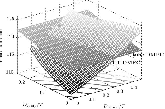
5.2 Effect of delays

Two different delays were introduced to the problem: Dcomp < T is the time delay between a

local agent’s measuring of its state and the subsequent updating of its control input (following optimization) during a time step of lengthT, whileDcomm< T is the time taken to successfully

communicate a new plan to other agents. For CT-DMPC, it is assumed that the pth agent may not optimize during step k until information is received from agent p−1 from earlier in the same interval (Richards and How 2007). Conversely, tube DMPC allows the whole interval [k+Dcomp, k+ 1) for communication.

For a two-mass system, with x1(0) = [5 1]T and x2(0) = [5 0]T, the delays Dcomp and Dcomm were varied over the intervals [0,0.25T] and [0,0.5T] respectively, where T = 1 second.

All parameters are the same as in the previous section, with the exception of the horizon, which was shortened toN = 7 to reflect the closer proximity to the origin of the initial states. During each simulation, disturbances were applied to force the masses apart: w1(k) = [1 1]T and w2(k) =−[1 1]T for all k.

Figure 3 compares the values of closed-loop cost obtained for both tube DMPC and CT-DMPC. As shown by the previous example, where no delays are present CT-DMPC achieves best performance. As delays are lengthened, the cost values for CT-DMPC are seen to increase, more severely so forDcomp. Where cost data are absent over the delay domain, the system violated

the constraints; CT-DMPC goes infeasible for Dcomp

T & 0.175 and additionally for high total

delayDcomp+Dcomm. On the other hand, the system controlled by tube DMPC achieves robust

feasibility over the whole domain. In addition, although higher than those of CT-DMPC for low values of delay, the cost values increase approximately linearly withDcomp and do not increase

withDcomm. Consequently, tube DMPC out-performs CT-DMPC when delays are longer. This

result confirms that CT-DMPC – with its reliance on instantaneous data exchanges – is the more susceptible of the two methods to the effect of delays, both in terms of feasibility and performance. Furthermore, it highlights a key feature of the tube DMPC method: that at least the full remainder of one time step is available for information exchange following an optimization.

6 Conclusions

0 1 0 8 :1 0 In ter n a ti o n a l J o u rn a l o f C o n tr o l d m p c˙ jn l Int e rna ti o na l J o u rna l o f C o nt ro l 1 3

Np= 2

∆x= 1

P

kNdata(k)

P k P p lp xp ( k ) , up ( k ) , × 1 0 3

0 5 10 15 20 25 30 35

3.9 4 4.1 4.2 4.3 4.4

Np= 3

∆x= 1

P

kNdata(k)

P k P p lp xp ( k ) , up ( k ) , × 1 0 3

0 20 40 60 80 100

6 6.2 6.4 6.6

Np= 4

∆x= 1

P

kNdata(k)

P k P p lp xp ( k ) , up ( k ) , × 1 0 3

0 50 100 150 200

7.8 8 8.2 8.4 8.6 8.8

Np= 2

∆x= 3

P

kNdata(k)

P k P p lp xp ( k ) , up ( k ) , × 1 0 3

0 5 10 15 20 25 30 35

3.9 4 4.1 4.2 4.3 4.4

Np= 3

∆x= 3

P

kNdata(k)

P k P p lp xp ( k ) , up ( k ) , × 1 0 3

0 20 40 60 80 100

6 6.2 6.4 6.6

Np= 4

∆x= 3

P

kNdata(k)

P k P p lp xp ( k ) , up ( k ) , × 1 0 3

0 50 100 150 200

7.8 8 8.2 8.4 8.6 8.8

Np= 2

∆x= 5

P

kNdata(k)

P k P p lp xp ( k ) , up ( k ) , × 1 0 3

0 5 10 15 20 25 30 35

3.9 4 4.1 4.2 4.3 4.4

Np= 3

∆x= 5

P

kNdata(k)

P k P p lp xp ( k ) , up ( k ) , × 1 0 3

0 20 40 60 80 100

6 6.2 6.4 6.6

Np= 4

∆x= 5

P

kNdata(k)

P k P p lp xp ( k ) , up ( k ) , × 1 0 3

0 50 100 150 200

7.8 8 8.2 8.4 8.6 8.8

Dcomm/T

Dcomp/T

cl

o

se

d

-l

o

o

p

co

st

←CT-DMPC

↑tube DMPC

0 0.1

0.2 0.3 0.4

0 0.1

0.2 110

115 120 125

Figure 3. Surfaces of closed-loop cost versus communication delayDcomm and computation delayDcomp. Contours are additionally shown for CT-DMPC.

communication is limited. Furthermore, a comparison with a similar robust distributed method has shown that the new algorithm offers a clear benefit, in terms of feasibility and performance, when computational and communication delays are present.

On-going research is investigating how to obtain closed-loop performance given a particular structure of coupling constraints. In particular, inter-agent cooperation may be employed – by including a consideration of other subsystems’ objectives in the local cost function – to promote system-wide performance by avoiding ‘greedy’ local decision-making.

References

Alessio, A., and Bemporad, A. (2007), “Decentralized Model Predictive Control of Constrained Linear Systems,” inProceedings of the European Control Conference, Jul, EUCA, pp. 2813– 2818.

Borrelli, F., Keviczky, T., and Stewart, G.E. (2005), “Decentralized Constrained Optimal Con-trol Approach to Distributed Paper Machine ConCon-trol,” in Proceedings of the 44th IEEE Conference on Decision and Control, and the European Control Conference, Dec, pp. 3037– 3042.

Camponogara, E., Jia, D., Krogh, B.H., and Talukdar, S. (2002), “Distributed Model Predictive Control,” IEEE Control Systems Magazine, 22, 44–52.

Du, X., Xi, Y., and Li, S. (2001), “Distributed Model Predictive Control for Large-Scale Sys-tems,” inProceedings of the American Control Conference, Jun, pp. 3142–3143.

Dunbar, W.B. (2007), “Distributed Receding Horizon Control of Dynamically Coupled Nonlinear Systems,”IEEE Transactions on Automatic Control, 52, 1249–1263.

Dunbar, W.B., and Murray, R.M. (2006), “Distributed Receding Horizon Control for Multi-Vehicle Formation Stabilization,” Automatica, 42, 549–558.

Franco, E., Magni, L., Parisini, T., Polycarpou, M.M., and Scattolini, R. (2008), “Cooperative Constrained Control of Distributed Agents with Nonlinear Dynamics and Delayed Informa-tion Exchange,” IEEE Transactions on Automatic Control, 53, 324–338.

Franco, E., Parisini, T., and Polycarpou, M.M. (2007), “Design and stability analysis of co-operative receding-horizon control of linear discrete-time agents,” International Journal of Robust and Nonlinear Control, 17, 982–1001.

Fukushima, H., and Bitmead, R.R. (2005), “Robust constrained predictive control using com-parison model,” Automatica, 41, 97–106.

planning for clusters of UUVs,” International Journal of Control, 80, 1169–1179.

Jia, D., and Krogh, B.H. (2002), “Min-Max Feedback Model Predictive Control For Distributed Control With Communication,” in Proceedings of the American Control Conference, May, pp. 4507–4512.

Keviczky, T., Borrelli, F., and Balas, G.J. (2006), “Decentralized receding horizon control for large scale dynamically decoupled systems,” Automatica, 42, 2105–2115.

Kim, T.H., and Sugie, T. (2005), “Robust Decentralized MPC Algorithm for a class of Dy-namically Interconnected Constrained Systems,” inProceedings of the IEEE Conference on Decision and Control.

Kolmanovsky, I., and Gilbert, E.G. (1998), “Theory and Computation of Disturbance Invariant Sets for Discrete-Time Linear Systems,”Mathematical Problems in Engineering, 4, 317–367. Kuwata, Y., Richards, A., Schouwenaars, T., and How, J. (2007), “Distributed Robust Reced-ing Horizon Control for Multivehicle Guidance,” IEEE Transactions on Control Systems Technology, 14, 627–641.

Ling, K.V., Maciejowski, J.M., and Wu, B. (2005), “Multiplexed model predictive control,” in

16th IFAC World Congress, Jul, Prague.

Maciejowski, J.M., Predictive Control with Constraints, Prentice Hall (2002).

Magni, L., and Scattolini, R. (2006), “Stabilizing decentralized model predictive control of non-linear systems,” Automatica, 42, 1231–1236.

Mayne, D.Q., Rawlings, J.B., Rao, C.V., and Scokaert, P.O.M. (2000), “Constrained model predictive control: Stability and optimality,” Automatica, 36, 789–814.

Mayne, D.Q., Seron, M.M., and Rakovi´c, S.V. (2005), “Robust model predictive control of con-strained linear systems with bounded disturbances,” Automatica, 41, 219–224.

Raffard, R.L., Tomlin, C.J., and Boyd, S.P. (2004), “Distributed Optimization for Cooperative Agents: Application to Formation Flight,” in Proceedings of the 43rd IEEE Conference on Decision and Control, pp. 2453–2459.

Richards, A., and How, J.P. (2005), “Implementation of Robust Decentralized Model Predic-tive Control,” in AIAA Guidance, Navigation, and Control Conference and Exhibit, Aug, American Institute of Aeronautics and Astronautics.

Richards, A., and How, J.P. (2007), “Robust Distributed Model Predictive Control,” Interna-tional Journal of Control, 80, 1517–1531.

Scattolini, R. (2009), “Architectures for distributed and hierarchical Model Predictive Control — A review,” Journal of Process Control, 19, 723–731.

Scokaert, P.O.M., and Mayne, D.Q. (1998), “MinMax Feedback Model Predictive Control for Constrained Linear Systems,” IEEE Transactions on Automatic Control, 43, 1136–1142. Shim, D.H., Kim, H.J., and Sastry, S. (2003), “Decentralized Reflective Model Predictive Control

of Multiple Flying Robots in Dynamic Environment,” in Proceedings of the 42nd IEEE Conference on Decision and Control.

Trodden, P.A. (2009), “Robust Distributed Control of Constrained Linear Systems,” PhD dis-sertation, University of Bristol.

Venkat, A.N., Rawlings, J.B., and Wright, S.J. (2004), “Plant-Wide Optimal Control With Decentralized MPC,” inProceedings of the 7th IFAC International Symposium on Dynamics and Control of Process Systems, Jul.

Venkat, A.N., Hiskens, I.A., Rawlings, J.B., and Wright, S.J. (2008), “Distributed MPC Strate-gies With Application to Power System Automatic Generation Control,”IEEE Transactions on Control Systems Technology, 16, 1192–1206.