Time-Varying Draft Restrictions:
A Case Study in Optimisation with
Time-Varying Costs
Elena Kelareva
A thesis submitted for the degree of
Doctor of Philosophy
The Australian National University
Many people helped me with this PhD research, both academically and by provid-ing support and advice along the way. First and foremost, I would like to thank my supervisors Sylvie Thiébaux, Philip Kilby and Mark Wallace for their invaluable advice, mentoring and support throughout my PhD.
Thanks also to Kevin Tierney, for collaborating with me on the paper which formed the basis of Chapter 7, as well as Sebastian Brand who came up with some of the ideas for CP model improvements in Chapter 4, and Tzameret Rubin, who helped me with some of the financial impact calculations in Chapter 5. I would also like to thank Charles Gretton and Julien Fischer for their assistance with some of the experiments in Chapter 7, and Olivia Smith for suggesting the idea of sequence variables discussed in Chapter 4.
Thanks also to the researchers in the maritime logistics research group at the Norwegian University of Science and Technology, whom I visited for a week and who gave me a great deal of useful feedback on my research, particularly Marielle Christiansen and Kjetil Fagerholt.
I would also like to thank my colleagues at OMC International, particularly Pe-ter O’Brien and Giles Lesser, who were instrumental in getting the ship scheduling project started and without whose support this research would never have been possible, as well as Gregory Hibbert, Kalvin Ananda, Gordon Lindsay, Andreas Schlichting, Mihir Mone, Lisa Solazzo, Sam Bao, Doug Leng and Jason Ryan, all
of whom contributed in various ways to the development of the DUKCR Optimiser
ship scheduling system discussed in Chapter 5.
I am also deeply grateful to my family and friends for helping to keep me sane through such a long project, particularly my mother, whose experiences with her own PhD were always a source of inspiration, as well as my husband, Rob, without whose support I probably would never have made it to the end. I would also like to thank my fellow PhD students and the Monday night games group at NICTA for being very welcoming and supportive during my visits to Canberra – you made completing my PhD as an external student a much more social experience.
Finally, this research was supported by the Australian government through an Australian Postgraduate Award, as well as by NICTA. NICTA is funded by the Aus-tralian Government as represented by the Department of Broadband, Communica-tions and the Digital Economy and the Australian Research Council through the ICT Centre of Excellence program.
In the last few decades, optimisation problems in maritime transportation have re-ceived increased interest from researchers, since the huge size of the maritime trans-portation industry means that even small improvements in efficiency carry a high potential benefit.
One area of maritime transportation that has remained under-researched is the impact of draft restrictions at ports. Many ports have restrictions on ship draft (dis-tance between the waterline and the keel) which vary over time due to variation in environmental conditions. However, existing optimisation problems in maritime transportation ignore time variation in draft restrictions, thus potentially missing out on opportunities to load more cargo at high tide when there is more water available for the ship to sail in, and more cargo can be loaded safely.
This thesis introduces time-varying restrictions on ship draft into several optimi-sation problems in the maritime industry. First, the Bulk Port Cargo Throughput Optimisation Problem is introduced. This is a novel problem that maximises the amount of cargo carried on a set of ships sailing from a draft-restricted bulk ex-port ex-port. A number of approaches to solving this problem are investigated, and a
commercial system – DUKCR Optimiser – based on this research is discussed. The
DUKCR Optimiser system won the Australia-wide NASSCOM Innovation Student
Award for IT-Enabled Business Innovation in 2013. The system is now in use at Port Hedland, the world’s largest bulk export port, after an investigation showed that it had the potential to increase export revenue at the port by $275 million per year.
The second major contribution of this thesis is to introduce time-varying restric-tions on ship draft into several larger problems involving ship routing and schedul-ing with speed optimisation, startschedul-ing from a problem involvschedul-ing optimisschedul-ing speeds for a single ship travelling along a fixed route, and extending this approach to a cargo routing and scheduling problem with time-varying draft restrictions and speed opti-misation.
Both the Bulk Port Cargo Throughput Optimisation Problem and the speed opti-misation research shows that incorporating time-varying draft restrictions into mar-itime transportation problems can significantly improve schedule quality, allowing more cargo to be carried on the same set of ships and reducing shipping costs.
Finally, this thesis also considers issues beyond time-varying draft restrictions in the maritime industry, and investigates approaches in the literature for solving optimisation problems with time-varying action costs. Several approaches are in-vestigated for their potential to be generalisable between different applications, and faster, more efficient approaches are found for both the Bulk Port Cargo Throughput Optimisation problem, and another problem in maritime transportation – the Liner Shipping Fleet Repositioning Problem.
Acknowledgments vii
Abstract ix
1 Introduction 1
1.1 Contributions . . . 2
1.2 Thesis Outline . . . 6
2 Background 9 2.1 The Maritime Transportation Industry . . . 9
2.1.1 Draft Restrictions at Ports . . . 12
2.1.2 Optimisation Problems in Maritime Transportation: Introduction 15 2.2 General Techniques . . . 15
2.2.1 Mixed Integer Programming . . . 16
2.2.2 Constraint Programming . . . 17
2.2.3 Planning . . . 19
2.2.4 Decomposition Techniques . . . 20
2.3 Optimisation Problems in Maritime Transportation . . . 20
2.3.1 Bulk Cargo Ship Routing and Scheduling . . . 21
2.3.2 Routing and Scheduling with Soft Time Windows . . . 24
2.3.3 Ship Speed Optimisation . . . 26
2.3.4 The Liner Shipping Fleet Repositioning Problem . . . 29
2.3.5 Draft Restrictions in Maritime Transportation Problems . . . 31
2.3.6 Summary . . . 32
3 Optimising Cargo Throughput at a Bulk Export Port 37 3.1 Introduction . . . 37
3.1.1 How Ship Sailing Times are Scheduled in Practice . . . 37
3.1.2 The Bulk Port Cargo Throughput Optimisation Problem . . . 38
3.1.3 BPCTOP Example . . . 40
3.1.4 Problem Features and Challenges . . . 41
3.2 Constraint Programming Model . . . 43
3.2.1 Variables and Parameters . . . 43
3.2.2 Constraints . . . 46
3.2.3 Objective Function . . . 47
3.3 Modelling Tugs . . . 47
3.3.1 Modelling Approaches . . . 48
3.3.2 Successful CP Model . . . 49
3.3.3 Tug Variables and Parameters . . . 51
3.3.4 Tug Constraints . . . 53
4 Scalability Improvements: Search Strategies and Alternative Models 55 4.1 Experimental Data . . . 55
4.1.1 Port Characteristics . . . 56
4.1.2 Problem Instances . . . 57
4.2 Search Strategies . . . 58
4.2.1 Draft vs Time Search . . . 59
4.2.2 Searching on Draft . . . 61
4.3 Mixed Integer Programming Model . . . 64
4.3.1 Variables and Parameters . . . 64
4.3.2 Constraints . . . 65
4.3.3 Tug Variables and Parameters . . . 66
4.3.4 Tug Constraints . . . 67
4.3.5 MIP vs CP Comparison . . . 68
4.4 Improvements to the Constraint Programming Model . . . 69
4.4.1 Sequence Variables and Time Search . . . 70
4.4.2 Other Improvements . . . 72
4.4.3 Search Strategies for the Improved CP Model . . . 73
4.5 Benders Decomposition . . . 76
4.5.1 Benders CP and MIP Models . . . 77
4.5.2 Experimental Results . . . 79
4.5.3 Alternative Benders Cuts . . . 80
4.5.4 New Benders CP Model . . . 80
4.5.5 Experimental Results for New Approach . . . 82
4.6 Summary . . . 83
5 Real-World Impact 85 5.1 The DUKC Optimiser System . . . 85
5.1.1 Initial Prototype . . . 85
5.1.2 User Interface . . . 86
5.1.3 Other Features . . . 88
5.1.4 System Architecture . . . 88
5.2 Schedule Quality Analysis . . . 89
5.2.1 Comparison Against Fixed Draft . . . 89
5.2.2 Comparison Against Manual Scheduling . . . 91
5.3 Comparison with Real Schedules . . . 95
5.3.1 Experimental Results . . . 96
5.4 Limitations and Future Work . . . 97
6 Ship Routing and Scheduling with Variable Speeds and Drafts 99
6.1 Introduction . . . 99
6.1.1 Calculating Shipping Costs . . . 99
6.1.2 Effect of Draft on Shipping Costs . . . 101
6.1.3 Existing Approaches to Cargo Routing with Variable Ship Speed 102 6.2 Speed Optimisation for a Fixed Route . . . 103
6.2.1 Problem Description . . . 103
6.2.2 Formal Problem Definition . . . 105
6.2.3 Shortest Path Approach . . . 106
6.2.4 Recursive Smoothing Algorithm . . . 107
6.2.5 Extending Norstad’s RSA for Multiple Time Windows . . . 108
6.2.6 Formal Algorithm Definition . . . 113
6.2.7 Smoothing Step . . . 115
6.2.8 Optimality of RSA . . . 119
6.2.9 Optimality of MW_RSA . . . 121
6.2.10 Scalability of Multi-Window RSA . . . 122
6.3 One Ship with Variable Draft . . . 125
6.3.1 Problem Instances . . . 126
6.3.2 Experimental Results . . . 127
6.4 Multiple Ships with Variable Draft . . . 132
6.4.1 Waypoint Cost Optimisation CP Model . . . 132
6.4.2 Solving the MS-SOPTVD . . . 133
6.4.3 Potential Algorithm Improvements . . . 134
6.4.4 Experimental Results . . . 137
6.5 Routing and Speed Optimisation . . . 140
6.5.1 Problem Description . . . 140
6.5.2 Our Approach . . . 142
6.5.3 Resolving Conflicts at Waypoints . . . 143
6.5.4 Experimental Results . . . 145
6.6 Summary . . . 149
7 Generalisation: Scheduling with Time-Varying Action Costs 151 7.1 Introduction . . . 151
7.2 Problems with Time-Varying Action Costs . . . 152
7.2.1 Satellite Imaging Scheduling . . . 153
7.2.2 Project Scheduling with Net Present Value . . . 154
7.2.3 Liner Shipping Fleet Repositioning . . . 155
7.2.4 Routing and Scheduling with Soft Time Windows . . . 156
7.2.5 Summary . . . 157
7.3 LSFRP . . . 158
7.3.1 Automated Planning and LTOP . . . 160
7.3.2 LSFRP LTOP Model . . . 160
7.3.3 MIP Model . . . 161
7.3.5 LSFRP CP Results . . . 167
7.4 Lazy Clause Generation . . . 170
7.4.1 Experimental Results for BPCTOP . . . 170
7.4.2 Experimental Results for LSFRP . . . 172
7.5 Solve-and-Improve . . . 174
7.5.1 Results for BPCTOP . . . 174
7.5.2 Results for LSFRP . . . 175
7.5.3 Summary . . . 175
7.6 Conversion to Vehicle Routing . . . 177
7.6.1 BPCTOP VRP Model . . . 177
7.6.2 Tug Constraints Model . . . 178
7.6.3 Experimental Results . . . 179
7.7 Summary . . . 181
8 Conclusion 183 8.1 Motivation . . . 183
8.2 Contributions . . . 183
8.2.1 Bulk Port Cargo Throughput Optimisation Problem . . . 183
8.2.2 Ship Speed Optimisation with Time-Varying Draft Restrictions . 184 8.2.3 Scheduling and Routing with Time-Varying Action Costs . . . . 186
8.3 Future Work . . . 187
2.1 Factors affecting under-keel clearance. . . 12
2.2 Ship squat [Barrass, 2004] . . . 13
2.3 Effect of ship heeling on under-keel clearance . . . 14
2.4 Vertical components of ship response to waves . . . 14
2.5 An example repositioning scenario with two vessels (solid and dashed black lines) reposition from their initial services to the goal service. . . 29
2.6 A subset of a real-world repositioning scenario, from Tierney et al. [2012a]. . . 30
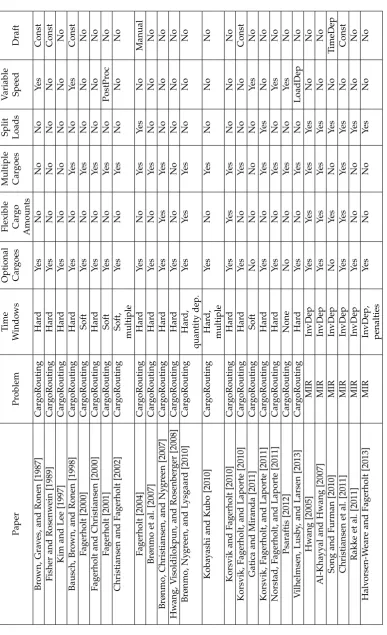
3.1 Port Hedland Layout . . . 40
3.2 Example Bulk Port Cargo Throughput Optimisation Problem . . . 41
3.3 Splitting a schedule of ships into scenarios for tug counting . . . 50
4.1 (a) Time search. (b) Draft search. . . 59
5.1 DUKCR Optimiser Output . . . 87
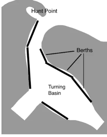
5.2 DUKCR Optimiser System Architecture . . . 88
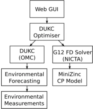
5.3 Schedule with time-varying draft vs. constant draft. . . 90
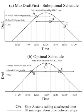
5.4 Manual schedule using ObjFunFirstvs optimal schedule. . . 92
5.5 Manual schedule using MaxDraftFirstvs optimal schedule. . . 94
6.1 Fuel cost, constant cost, and total cost for travelling a fixed distance with a range of ship speeds (in knots). . . 100
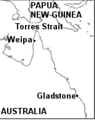
6.2 Map of Weipa – Torres – Gladstone shipping route. . . 104
6.3 RSA Step 1: Calculate optimal speed for route, ignoring time windows except at first and last waypoints. Then find waypoint with largest time window violation and adjust its arrival time to the nearest feasible time. . . 107
6.4 RSA Step 2: Split route at waypoint with largest time window violation and recalculate subroutes recursively. . . 108
6.5 MW_RSA Step 1: Try splitting the route on both the waypoint with the largest distance to the previous time window, and the waypoint with the largest distance to the next time window. Try adjusting the time at the selected waypoint to both the nearest feasible times before and after the original optimal time. . . 110
6.6 MW_RSA Step 2: After adjusting arrival time at selected waypoint, split the route at that waypoint, and recursively optimise both sub-routes until all arrival times at waypoints are within valid time win-dows. In this case, both subroutes WP1 – WP3 and WP3 – WP5 will need to be adjusted further. . . 111
6.7 Example showing why both the waypoints with the largest time
win-dow violations before and after need to be considered for splitting the route. WP2 has the largest time window violation overall; however, if only WP2 is considered for splitting, the valid window at WP3 will not be found. . . 112
6.8 WP3 has the largest distance to the previous time window, and
con-sidering both WP2 and WP3 finds the optimal route. . . 112
6.9 Example showing why a final smoothing step is required. WP2 or
WP4 would be chosen first for splitting; however both result in a sub-optimal route, as the sub-optimal path passes through the middle of time windows at both WP2 and WP4. A smoothing step is required to re-move unnecessary speed changes. . . 117 6.10 Illustration for RSA proof of optimality. . . 120 6.11 Illustration for RSA proof of optimality – 2 cases. . . 120 6.12 Minimum voyage cost and opportunity cost for 20 discretised draft
values. . . 128
7.1 Cost increase of optimal and VRP solutions compared to all ships
2.1 Routing and scheduling problems in bulk shipping. All involve rout-ing between multiple ports. . . 33
2.2 Other maritime optimisation and vehicle routing problems . . . 34
4.1 ObjFun vs Draft vs Time search – number of ships in the largest
problem solved within the cutoff time, with CPU time in seconds in brackets. . . 61
4.2 ObjFunsearch – number of ships in the largest problem solved within
the cutoff time, with CPU time in seconds in brackets. . . 62
4.3 Draftsearch – number of ships in the largest problem solved within
the cutoff time, with CPU time in seconds in brackets. . . 62
4.8 Largest problem solved, with solution time in seconds for MIP vs CP. . 69
4.9 Search strategies on the time dimension - largest problem solved, with
CPU times in seconds. . . 71 4.10 Comparison of original vs modified CP models - largest problem solved,
with CPU time in seconds. . . 73 4.11 Comparison of search strategies for the CP model with all three
im-provements. . . 74 4.12 Searching by draft vs sequence variables for improved model with
one-dimensional arrays only. . . 74 4.13 Searching by draft vs sequence variables for improved model with
sorted ships only. . . 75 4.14 Benders CP and MIP models vs. combined CP model – largest problem
solved for each type, with corresponding CPU time in seconds. . . 79 4.15 MIP vs CP models for the Benders Master and Subproblems – CPU
times for the final iteration in seconds. . . 79 4.16 Benders approach with separation time cuts vs. tug cuts and the
com-bined CP problem – CPU time in seconds. . . 82 4.17 Number of iterations and CPU times in seconds for the final iteration
of the master problem for the largest problem solved by Benders with tug cuts vs. separation time cuts. . . 82
6.1 RSA: worst-case number of speed optimisation calculations vs. average
over 8 ships x 20 drafts vs. worst-case seen over 8 ships x 20 drafts. . . . 124
6.2 Calculation time in seconds for optimising speeds for 8 ships x 20
drafts, for MW_RSA vs Shortest Path approach. . . 124
6.3 Distances between waypoints for 16-waypoint route, in nautical miles. . 127
6.4 Percentage by which Shortest Path cost with 20, 40, 60, 80 and 100 arrival time discretisations exceeds RSA cost, averaged over 8 ships. . . 128
6.5 Percentage cost improvement of optimal draft vs. unconstrained draft,
using RSA for speed optimisation, averaged over 8 ships. . . 129
6.6 Percentage reduction in cost of considering draft constraints in speed
optimisation vs. ignoring draft windows in speed optimisation and waiting when ship arrives outside the windows, for same (optimal) draft. Averaged over 8 ships. . . 130
6.7 Percentage reduction in cost of considering draft constraints in speed
optimisation vs. ignoring draft windows in speed optimisation and waiting when ship arrives outside the windows, for same (optimal) draft, when ships do not sail faster to catch up. Averaged over 8 ships. 130
6.8 Cost improvement of considering draft restrictions in speed
optimisa-tion vs. ignoring draft restricoptimisa-tions and waiting, for a ship with fixed drafts with different minimum time windows at waypoints. Averaged over 8 ships. . . 131
6.9 Percentage increase in cost for schedule with resource constraints at
waypoints vs. lower bound ignoring resource conflicts computed with RSA. . . 138 6.10 Percentage cost increase for MS-SOPTVD with initial 1-ship solutions
calculated using 60-time-discretisation Shortest Path vs. RSA. . . 139 6.11 Percentage reduction in cost caused by considering resource conflicts
at waypoints, rather than optimising speeds for individual ships using RSA, and waiting at waypoints in the event of resource conflicts. . . 139 6.12 Percentage reduction in cost for 8-ship problems caused by
consider-ing draft constraints and resource conflicts at waypoints vs. ignorconsider-ing draft windows in speed optimisation for drafts with different mini-mum time windows at waypoints. Averaged over 8 ships. . . 140 6.13 Comparing different approaches for the instance with 4 multi-ship
car-goes, 4 ships and a 4-port map. . . 146 6.14 Average percentage difference in profit for different strategies,
com-pared against sailing at service speed, averaged over 16 problem in-stances for each number of cargoes. . . 148
7.1 Characteristics of problems reviewed in the literature. . . 159
7.4 Computation times to optimality in seconds with a timeout of one
hour for the CP model with and with annotations (A), repositioning type order (O), and redundant constraints (R) versus LTOP and the MIP.169
7.5 CPU time (s) for CPX solver with LCG vs. G12 finite domain solver on
OneWay_Narrow(ON) problems. . . 171
7.6 CPX solver vs. G12 finite domain solver: number of ships in the largest
7.7 Computation times to optimality in seconds with a timeout of one hour for the CP model without LCG (CP–AOR) and with LCG (CPX–AOR). . 173
7.8 Runtime (s) of CPX vs. the FD solver with a simplified BPCTOP model. 174
7.9 Computation times to optimality in seconds for CP and LTOP versus
simplified approaches (S–LTOP and S–CP–AOR) with optimal win-dows. Note that we have removed all TP7 instances except for TP7_6_0 due to timeouts. . . 176 7.10 Indigo VRP solver vs. G12 FD and CPX solvers, without tug
Introduction
Maritime transportation is one of the most important forms of freight transportation, with over 8 billion tonnes of goods per year transported by sea [UNCTAD, 2011]. With the huge volumes of goods being transported, there is a high potential for cost optimisation in the maritime shipping industry. There has been significant interest in recent years on optimisation problems in maritime logistics, but this area is still under-researched compared to land and air transportation, as discussed in two recent reviews of the maritime transportation literature: Christiansen, Fagerholt, and Ronen [2004] and Christiansen et al. [2013]. Though maritime shipping has been tradition-ally a conservative industry, computerised decision support systems are beginning to be more frequently accepted as their benefits are becoming more clear [Fagerholt, 2004].
This thesis investigates several optimisation problems in the maritime transporta-tion field, particularly focussing on scheduling and routing problems. Scheduling problems typically aim to select execution times for a set of tasks so as to optimise some cost or value function, subject to problem-specific constraints, particularly on the availability of resources such as machines. Traditional scheduling problems usu-ally aim to minimise the makespan, or total time, of the resulting schedule, though more complex cost functions have also been investigated.
Routing problems have many similarities with scheduling – both have actions that need to be scheduled in time, both may have resource constraints and constraints on setup (waiting) time between actions, and both have some cost function that needs to be optimised. However, the pickup and delivery tasks being scheduled in a routing problem have durations that depend on the relative locations of pickup and delivery nodes in space, and thus vary with the order of actions, whereas in a pure scheduling problem, action durations are generally fixed and do not depend on order, though some scheduling problems do involve sequence-dependent setup times between ac-tions.
Optimisation problems in the maritime transportation domain typically focus on minimising the cost or maximising the profit of some aspect of maritime industry operations, such as the cost required to transport a fixed amount of cargo, or the profit obtained by a shipping company. Alternative objectives may include max-imising the utilisation of a costly resource such as berths at a port, minmax-imising fuel usage and carbon dioxide emissions, or optimising customer satisfaction. These
jectives are similar to those found in ground, rail and air transportation; however, the constraints involved in maritime shipping may differ substantially. The large value of even a small percentage reduction in global shipping costs makes maritime transportation problems an area of great potential for future research.
One consideration in maritime logistics which does not occur in other modes of transportation is that most ports have restrictions on the draft of ships that are able to safely enter and leave the port. Draft is the distance between the waterline and the bottom of the ship’s keel, and is a function of the amount of cargo loaded onto the ship. Ships with a deep draft may risk running aground in shallow water, therefore most ports restrict ship sailing drafts using safety rules that estimate the under-keel clearance (UKC) – the depth of water under a ship’s keel.
These safety rules are dependent on environmental conditions such as tide, waves and currents, and therefore in practice, the allowable sailing draft at most ports varies with time. Existing ship scheduling algorithms either ignore draft constraints entirely, for example Fagerholt [2004]; Norstad, Fagerholt, and Laporte [2011], or only consider draft constraints that are do not vary with time [Christiansen et al., 2011; Rakke et al., 2011]. This may result in suboptimal solutions, where ships sail with less cargo than they could have carried if the algorithm had considered the possibility of sailing with a higher draft at high tide.
This dissertation investigates the question: what is the impact of considering draft restrictions on ship scheduling?
The main thesis of this dissertation is that accurate consideration of time-varying draft restrictions in maritime transportation problems can result in reduced shipping costs or increased cargo throughput by taking advantage of the opportunity to load more cargo at high tide. We introduce time-varying draft restrictions into a number of maritime transportation problems, and show that this approach can significantly reduce shipping costs, as well as increase revenue for shippers by allowing more cargo to be transported on the same set of ships.
1
.
1
Contributions
There are three main areas of contribution consisting of three main novel problems investigated in this thesis:
1. Introducing the novel Bulk Port Cargo Throughput Optimisation Problem (BPC-TOP) with time-varying drafts, and investigating a number of approaches to solving it.
2. Adding time-varying draft restrictions to the ship routing and scheduling prob-lem with speed optimisation.
3. A more general investigation of scheduling and routing problems with time-varying cost functions in related fields.
Optimisation Problem (BPCTOP). This problem is motivated by a real port – Port Hedland in Western Australia, the world’s largest bulk export port, which is draft-restricted and has up to six metres difference between high and low tides, and can therefore benefit significantly from optimising ship schedules with draft restrictions taken into account.
The Bulk Port Cargo Throughput Optimisation Problem involves scheduling ship sailing times at only one port; however, even at one port, this is quite a challenging problem, since it involves complex resource constraints and interactions between ships. The high tidal variation means that the draft changes significantly even in as short a time as five minutes. Since the allowable sailing draft for a ship cannot be specified by any simple equation, the problem needs to be modelled using a very fine time-indexed formulation. Typical ship scheduling and routing problems can be modelled with a time resolution of hours or even days; however, introducing time-varying drafts requires increasing the resolution to intervals on the order of five minutes, resulting in large domains for the decision variables, and making the problem more difficult to solve.
We create a Constraint Programming model for the BPCTOP and investigate a number of approaches to modelling different aspects of the problem. One part of the problem that is particularly challenging to model is the constraints on the availability of tugs – small boats that are used to assist ships entering and leaving the port. Tug constraints are very complex, since the minimum duration of a tug’s action in assisting a ship depends on the destination of the current ship, as well as the origin of the next ship, since travel time between these locations needs to be taken into account. We considered three approaches to modelling tugs, and were able to take advantage of features of the problem to simplify tug constraints and create a tractable model that was able to solve realistic sized problems within five minutes. The CP model is also compared against a Mixed Integer Programming model, with the finding that a CP solver with a good choice of search strategy is able to prove optimality faster for most problem instances.
While these results are quite solver- and problem-specific, the broader implication of these results is that Constraint Programming approaches for solving new problems should consider the choice of model, solver and user-defined search strategy as an interacting system, rather than in isolation, as the calculation speed is affected by the interaction between these three factors. The results of our investigation into CP model improvements and user-defined search strategies for the BPCTOP also suggests a number of improvements for the G12 finite domain CP solver which we use to solve the CP model for the BPCTOP.
The best CP model with the fastest user-defined search strategy has been
incorpo-rated into a commercial system for scheduling ships at a port – DUKCR Optimiser.
This system is now in use at Port Hedland in Western Australia, the world’s largest
bulk export port, after comparisons of DUKCR Optimiser results against schedules
produced by human schedulers at Port Hedland showed that the system had the potential to increase export revenue at the port by US$275 million per year. These
comparisons of DUKCR Optimiser results against real schedules from Port Hedland
are presented in Chapter 5, along with a few simple examples to illustrate why the system is able to find schedules which allow ships to carry more cargo compared
to approaches typically used by human schedulers. The DUKCR Optimiser system
was awarded the NASSCOM Innovation Student Award for IT-Enabled Business In-novation in 2013 [Consensus Group, 2013].
Chapter 6 presents the second main contribution of this thesis by introducing time-varying draft restrictions into a larger bulk ship routing and scheduling prob-lem with speed optimisation, building on the work of Norstad, Fagerholt, and La-porte [2011], who investigated ship speed optimisation for a bulk ship routing and scheduling problem. Optimising ship sailing speeds has been widely investigated in recent years, since rising fuel prices have made fuel costs comprise a larger pro-portion of total shipping costs, and fuel usage is a function of ship speed. How-ever, draft restrictions affect allowable sailing windows at ports and draft-constrained waypoints, which may affect the optimal speed for ships. It is therefore worthwhile to consider these two aspects of ship scheduling in combination.
We start by incorporating time-varying draft restrictions into a simple subprob-lem – speed optimisation for a single ship travelling along a fixed route. We extend the recursive smoothing algorithm introduced by Norstad, Fagerholt, and Laporte [2011] to be able to handle our more complex problem, with multiple time windows, one around each high tide, as well as a non-monotonic cost function that takes into account not only fuel usage, but also ship draft as well as the opportunity cost of not being able to use the ship for other voyages if the duration of the current voyage takes longer due to sailing at a slower speed. We compare our approach against an alternative way of handling draft restrictions – having the ship wait at draft-restricted waypoint until the tide rises high enough for it to sail – and find that considering time-varying draft restrictions in ship speed optimisation reduces costs by an average of 22%.
bulk ship routing and scheduling problem with speed optimisation and time-varying draft restrictions. We compare four ways of solving this problem:
1. Considering both time-varying draft restrictions and resource conflicts between ships at waypoints in speed optimisation.
2. An approach that considers time-varying draft restrictions in the speed opti-misation problem but ignores resource conflicts between ships, thus requiring ships to wait for each other to sail.
3. Ignoring draft restrictions in speed optimisation and having ships wait for the tide to rise if required, as well as waiting for other ships to sail.
4. Sailing at a fixed service speed and waiting at waypoints for the tide to rise as well as for other ships.
Considering time-varying draft restrictions in speed optimisation results in a 22% reduction in shipping cost on average for our problem instances compared to sailing at a fixed service speed. The method presented by Norstad, Fagerholt, and Laporte [2011] of optimising speeds without considering draft constraints and resource con-flicts at waypoints results in a 15% reduction in shipping cost compared to sailing at service speed. Considering resource conflicts at waypoints resulted in a small additional reduction in cost, about 2% more than speed optimisation with time-varying draft restrictions alone. These results show that considering time-time-varying draft restrictions in maritime optimisation problems can result in a substantial bene-fit to industry, and we hope that more maritime logistics researchers will incorporate time-varying draft restrictions into their models in future.
The third main contribution of this thesis is to look beyond the specific problem of time-varying draft restrictions in maritime optimisation, to consider the more general problem of scheduling and routing with time-varying costs. The time-varying cost function is one of the main sources of complexity for the problems considered in this thesis. Other routing and scheduling problems in related fields have also considered time-varying action costs, so the final chapter in this thesis summarises how related problems in other fields have dealt with time-varying costs, and investigates the potential of generalising some of these approaches between different applications.
even though, as discussed earlier, the performance of Constraint Programming ap-proaches is highly dependent on the choice of model, solver and search strategy.
We also investigate the effectiveness of a new CP solver on both the LSFRP and BPCTOP. This solver uses Lazy Clause Generation, a recently introduced technique which allows a CP solver to learn areas of the search space where no good solutions have previously been found, and speed up the search by avoiding them in future. We find that the LCG solver outperforms traditional finite domain CP solvers on both the LSFRP and BPCTOP.
We also compare the CP model and LCG solver for our problems against a more typical approach to speeding up calculation of a problem with time-varying costs – a solve-and-improve method which first solves a simplified version of the problem without time-varying costs, then uses the real cost function to improve the solution. We find that, while the simplified models for both problems are faster to solve than the original approach, the speed improvement provided by the solve-and-improve method is lower than that obtained by the CP model for the LSFRP and the LCG solver for the BPCTOP.
Finally, we investigate a novel approach to solving the BPCTOP by modelling it as a Vehicle Routing Problem with Soft Time Windows (VRPSTW) and using an existing fast VRP solver to solve this problem. We find that modelling a scheduling problem as a VRP can be an efficient way to get good quality solutions, though the VRP solver has limitations on the kinds of constraints that can be modelled, which limits the types of scheduling problems that can be solved using this approach, and in the case of the BPCTOP, limits the accuracy of the resulting solutions.
These results show that there is scope for generalisation of approaches between scheduling and routing problems with time-varying costs in related fields, and fur-thermore, that some approaches such as Constraint Programming and Lazy Clause Generation can outperform methods traditionally used for such problems such as Mixed Integer Programming.
1
.
2
Thesis Outline
This thesis is formatted as follows.
• Chapter 2 introduces the reader to the maritime transportation industry and
• Chapter 3 introduces the Bulk Port Cargo Throughput Optimisation Problem with time-varying draft restrictions. We present a Constraint Programming (CP) model for this problem, and discuss a number of approaches for modelling the most complex part of this problem – constraints on the availability of tugs.
• In Chapter 4, we investigate the scalability of our CP model for realistic problem
sizes, and we compare a number of search strategies for solving this model. We also compare our CP model against a Mixed Integer Programming (MIP) model for this problem, as well as against a Benders Decomposition approach that breaks the model up into a master and subproblem, both of which can be implemented as either CP or MIP models. Finally, this chapter investigates a number of variations on our initial CP model aimed at improving scalability.
• In Chapter 5, we discuss DUKCR Optimiser, the commercial software system
for scheduling ship sailing times that has been implemented based on our
BPC-TOP models. Comparisons of DUKCR Optimiser results against human
sched-ulers on real data are also presented in this chapter.
• Chapter 6 incorporates time-varying draft restrictions into two more problems
in maritime logistics – the problems of ship speed optimisation for a single ship travelling along a fixed route, and the problem of ship scheduling and routing with variable speeds and time-varying draft restrictions. We compare our re-sults for both problems against approaches that optimise speed while ignoring time-varying draft constraints, as well as against traditional approaches that ignore draft and use fixed ship speeds.
• In Chapter 7, we consider our work in the more general context of scheduling
and routing problems with time-dependent cost functions, and compare several approaches that have been used to solve related problems in other fields. We also investigate the effectiveness of several of these approaches for a related problem with time-dependent costs – the Liner Shipping Fleet Repositioning Problem (LSFRP). The LSFRP is a problem first introduced by Kevin Tierney, and the sections on the LSFRP presented in this chapter are joint work with Kevin Tierney. Other chapters are primarily the author’s work, with feedback and suggestions from numerous people as listed in the acknowledgements.
• Chapter 8 presents concluding remarks and several avenues for future work
arising from this research.
Parts of this thesis have previously been published as:
• Kelareva et al. [2012b] – short conference paper; brief summary of Chapter 3
and parts of Chapter 4.
• Kelareva et al. [2012a] – Chapter 3 and parts of Chapter 4.
• Kelareva [2012] – parts of Chapter 5.
• Kelareva et al. [2013] – short conference paper; brief summary of parts of
Chapter 6.
• Kelareva, Tierney, and Kilby [2013a] – parts of Chapter 7.
Background
This chapter presents an overview of optimisation problems in the maritime trans-portation industry, as well as several general techniques commonly used to solve these types of problems which are also used in this thesis. This chapter also dis-cusses how draft restrictions at ports are calculated in practice, as well as how draft restrictions in maritime transportation problems have been considered in the existing literature.
This chapter is not an exhaustive survey of the maritime transportation literature; in particular, only a few problems in container shipping are discussed, as this thesis focusses primarily on problems in bulk cargo shipping. The section on general op-timisation techniques written as an introduction for readers unfamiliar with any of the approaches used in this thesis, and is not intended as an exhaustive survey of the field of optimisation.
2
.
1
The Maritime Transportation Industry
Cargo and shipping service types
Commercial shipping services fall into three distinct types – tramp, industrial and
liner.
Alinershipping service operates similarly to a bus timetable, with several vessels travelling along a fixed route with a fixed timetable. Liner services are typically used for containers and general cargo. Roll-on Roll-off (RoRo) vessels used to transport cars and other rolling equipment are also typically part of a liner shipping service.
Tramp ships operate similarly to a taxi company, with tramp ships taking up
contracts of affreightmentto transport a specified amount of cargo from an origin to a destination port within a fixed timeframe for a given price. Tramp ships are typically used for bulk cargo, and a tramp operator typically tries to maximise the profit produced by the fleet of ships.
Industrial ships are either owned by the cargo owner, or hired on a time charter
for a fixed period of time. Industrial ships are typically used for high-volume bulk cargoes such as oil, coal and iron ore.
All three types of cargo ship operators are able to charter additional vessels if required to meet excess demand, or charter out their own vessels in the event of fleet
capacity exceeding demand.
Non-commercial vessels such as naval vessels are not considered in this thesis, as they involve quite different problems compared to commercial cargo shipping.
Ships
Ships come in many different sizes, with differing speeds and fuel usages, as well as capacities of weight and volume of cargo. Ships are also limited in the types of
cargo they can carry – tankers carry liquid bulk cargo; bulk carriers carry dry bulk
such as wheat, timber or ore;containerships carry standard-sized containers used for
transporting packaged goods; Roll-on Roll-off(RoRo) ships are used for transporting
cars or other rolling equipment. Other types of ships include refrigerated vessels used to transport cargo that requires refrigeration such as meat or vegetables, and Liquefied Natural Gas (LNG) carriers, used to carry pressurised, refrigerated gas. Bulk ships may be able to carry either one type of cargo, or several types of cargo in separate compartments, possibly with constraints on the types of cargo that may be transported in each compartment, or the types of cargo that may be stored adjacent to each other.
Ship sizes vary significantly, with ships falling into several main size classes based on their dimensions and deadweight tonnage (DWT) – the total weight the ship can safely carry, including all extras such as fuel, ballast and crew. The most commonly used size categories for dry cargo as listed in the UNCTAD [2012] Review of Mar-itime Transport and Rodrigue, Comtois, and Slack [2013] are:
1. Handysize– small bulk carriers, mostly used for minor bulk products and small ports. 10,000 – 34,999 DWT.
2. Handymax– slightly larger than Handysize: 35,000 – 54,999 DWT.
3. Panamax– the largest ship size that can travel through the Panama canal: 55,000
– 84,999 DWT; breadth< 32.31m. This size class is used for both bulk carriers
and tankers.
4. Capesize – large bulk cargo vessels that are too large to pass through the Suez and Panama canals and must thus travel around the Cape of Good Hope or Cape Horn to travel between oceans. These vessels are only able to serve ports with deepwater terminals, and are primarily used to transport raw materials such as iron ore and coal. The size range is defined slightly differently in different sources [UNCTAD, 2012; Rodrigue, Comtois, and Slack, 2013], but
generally includes ships larger than Panamax, ie. 80,000+ DWT, breadth >
32.31m.
5. Very Large Ore Carrier / Ultra Large Ore Carrier – 200,000+ DWT and 300,000+ DWT respectively; used for transporting iron ore from Brazil. Only a few ports worldwide can accommodate vessels of this size.
1. Aframax– 80,000 – 124,999 DWT, larger than Panamax.
2. Suezmax– the largest ship size that can travel through the Suez canal, 125,000 – 199,999 DWT.
3. Very Large Crude Carrier– 200,000 – 320,000 DWT. Can dock at many terminals, and can be ballasted through the Suez Canal.
4. Ultra Large Crude Carrier– 320,000+ DWT; can only dock at a few terminals.
Several other ship size classes are the Seawaymax – the largest ships able to pass
through the St Lawrence Seaway;Q-MaxorQatar-max– the largest LNG carriers able
to dock at the Qatar LNG terminal; and Malaccamax – the largest ships able to sail
through the Malacca Strait.
Different ship types and size classes may be subject to different port charges, as well as variations in safety rules at ports. For example, at Port Hedland in West-ern Australia, vessel berthing charges depend on the length of the vessel, and pi-lotage charges depend on the total deadweight tonnage [Port Hedland Port Author-ity, 2013a]. Different vessel size classes also have different safety requirements for the number of tugs that must assist the vessel in arriving or departing a berth, and in entering or leaving the port [Port Hedland Port Authority, 2013c].
Ports
Ports vary in their geography and environmental conditions, which may affect safety requirements for ships operating in and around the port, including restric-tions on draft. Each port has a number of berths, with different dimensions and loading/unloading equipment, which may limit the size and type of ships that can use each berth. Different loading and unloading equipment may also have varying loading and unloading rates. Some ports are used for both pickup and delivery of cargo; many other ports, particularly in the bulk shipping industry, are used almost exclusively for one or the other.
Some ports or berths may be privately owned, and thus reserved for use by ships owned or chartered by one company; other berths are public, and may be shared by ships operated by many different companies, with the port charging fees for docking, refueling, and other services. The port typically aims to minimise the turnaround time of ships using the port, as cycling ships through faster increases utilisation of port facilities and thus port revenue. Ports may also aim to maximise the total cargo throughput, particularly if they charge fees per tonne of cargo shipped.
One issue that is of importance to ports is queueing rules used to determine the order in which ships may dock. Many ports use a first-come first-served queueing system, which is simple to administer, but which results in ships sailing quickly to reach the port, followed by waiting for up to several weeks in the queue outside the port. This is highly inefficient, as ships sit idle for weeks at a time, when they could have sailed slower and used less fuel.
Figure 2.1: Factors affecting under-keel clearance.
transportation equipment such as ship loaders, cranes and container transport vehi-cles, cargo storage facilities, and other equipment such as pilot boats used to trans-port harbour pilots to inbound vessels, and lines boats used to assist in mooring ships at a berth. Capacity planning for ports is therefore an important and complex problem, since projects to extend the capacity of a port by extending the infrastruc-ture, for example by building additional berths or dredging the channel to increase the allowable ship drafts, can cost billions of dollars [BHP Billiton, 2011]. Optimisa-tion and other software systems that improve the utilisaOptimisa-tion of existing port capacity may also be installed to increase the extra port capacity provided by such projects.
2.1.1 Draft Restrictions at Ports
Draft is the distance between the waterline and the ship’s keel. Most ports have safety restrictions on the draft of ships allowed to transit through the channel to reduce the risk of deep-draft ships running aground in shallow water. At draft-restricted ports, accurate modelling of draft constraints allows more cargo to be loaded onto each ship in good environmental conditions without compromising safety, which increases profit for shipping companies. In practice, draft constraints at ports are usually calculated by estimating the under-keel clearance of a ship – the amount of water under the ship’s keel.
The equations used to calculate under-keel clearance calculations vary between ports. Some ports use simple static estimates of under-keel clearance, which do not consider any live measurements of environmental conditions, and which must there-fore be very conservative to maintain safety. In recent years, some ports have begun to use more sophisticated systems which incorporate live environmental forecasts and measurements to produce more accurate estimates of under-keel clearance, and therefore can allow ships to sail with a higher draft on average, while maintaining
safety. The Dynamic Under-Keel Clearance (DUKCR) software developed by OMC
Figure 2.2: Ship squat [Barrass, 2004]
Factors which affect the under-keel clearance of a ship (shown in Figure 2.1) include:
• thedepth of water at each point along the channel.
• the predicted tide height at the time the ship will be transiting through the
channel.
• thedraftof the ship.
• squat– a phenomenon caused by the Bernoulli effect, which causes a ship trav-elling faster in shallow water to sit lower in the water, as illustrated in Fig-ure 2.2 [Barrass, 2004].
• heel– the effect of a ship leaning to one side under the effect of centripetal force
due to turning, or due to the force of wind. Heel causes one side of the ship to sit lower in the water, thus decreasing under-keel clearance, as illustrated in Figure 2.3.
• wave response– the vertical component of a ship’s motion in response to waves, as illustrated in Figure 2.4.
Other factors may play a part at specific ports, for example, the changing density of water may affect under-keel clearance at estuary ports where the salinity, and therefore density, of the water varies at different locations along the channel, and at different times in the tide cycle. See O’Brien [2002] for a detailed overview of under-keel clearance at ports.
Equation (2.1) shows an example under-keel clearance constraint for a port. A
vesselv will be allowed sail at time tif the constraint expressed in Equation (2.1) is
Figure 2.3: Effect of ship heeling on under-keel clearance
Figure 2.4: Vertical components of ship response to waves
the sum of the negative UKC factors (draft d, squat s, heel h, wave response w, etc)
exceeds some safety factorF.
D(t) +T(t)−d(v)−s(v,t)−h(v,t)−w(v,t)≥ F (2.1)
2.1.2 Optimisation Problems in Maritime Transportation: Introduction
Optimisation problems in maritime transportation are traditionally divided into three
levels: strategic, tacticalandoperational, based on the time-frame of decision-making.
However, there is substantial overlap between these levels, partly because of unclear boundaries between them, and partly because even high-level problems like fleet size and mix or port capacity planning will depend on the details of the day-to-day demand for the resources in question.
Strategic planning problems include port capacity planning; optimisation of ship-ping fleet size and mix; liner shipship-ping service and network design; and supply chain design.
Tactical planning problems include bulk cargo routing and scheduling; liner fleet deployment – the process of assigning ships to liner shipping routes; the Liner Ship-ping Fleet Repositioning Problem (LSFRP), which aims to minimise the cost of mov-ing a ship between different liner routes; the Berth Allocation Problem; and the Maritime Inventory Routing (MIR) problem – the combined problem of coordinat-ing inventory at various stages of a supply chain, as well as minimiscoordinat-ing the cost of routing cargo.
The boundary between tactical and operational planning problems is often un-clear, but some problems clearly fall into the short-term operational planning hori-zon. These include environmental routing – the process of choosing routes that avoid floating ice or poor weather conditions, or take advantage of ocean currents to re-duce fuel usage or travel times; and problems involving ship speed selection aimed to minimise fuel costs or emissions from shipping.
Section 2.2 provides an introduction to a number of general techniques that are used in this thesis, which are commonly used in maritime transportation problems as well as in related optimisation problems in other fields. Section 2.3 then discusses a few key optimisation problems in maritime transportation in more detail, partic-ularly problems in bulk cargo ship routing and scheduling that are most closely related to the research presented in this thesis.
2
.
2
General Techniques
planning problems, so methods for solving planning problems are also briefly pre-sented.
2.2.1 Mixed Integer Programming
Mixed Integer Programming involves minimising or maximising a linear function subject to linear constraints. Specifically, a Mixed Integer Program has the form:
minimisecTx (2.2)
subject to Ax=b
l≤ x≤u
some or allxj are integers
Mixed Integer Programs are typically solved using abranch-and-boundapproach [Land
and Doig, 1960]:
1. Continuous (Linear Programming) relaxation: allow all x to take non-integer
values, and find the optimal real solution for both branches. If this solution gives integer values for all variables that are required to be integers, then we are done. Otherwise, do steps 2-4.
2. Branch: find a variable xj that is required to be an integer, which has a
non-integer value in the LP solution, say vj. Create two new subproblems, one
with the added constraint xj ≤ bvjc, and the other with the added constraint
xj ≥ dvje.
3. Bound: the solution to the LP relaxation provides a lower bound on the solution to the MIP problem. Any feasible integer solution found so far provides an upper bound, which is updated during the search as better solutions that satisfy integrality constraints are found. These upper and lower bounds can be used to prune branches during the search: if the lower bound for any branch is above the upper bound found so far, that branch cannot provide any better quality solutions, and can be pruned.
4. Solve subproblems: recursively solve the two subproblems created by branch-ing usbranch-ing steps 1-4, until either a) the optimal solution to the continuous re-laxation is infeasible, or b) the optimal solution to the continuous rere-laxation satisfies integrality constraints, or c) the branch can be pruned by step 3. Other methods used for solving Mixed Integer Programs include:
1. The cutting planes method, which repeatedly finds optimal solutions under a
continuous relaxation and adds additional inequalities orcutsto separate
non-integer optimal solutions away from the feasible set.
3. Column generation, a method for solving large Mixed Integer Programs that would be infeasible to solve directly, by considering only a subset of variables at a time, repeatedly adding new variables (columns) that can improve the solution.
4. Dantzig-Wolfe decomposition [Dantzig and Wolfe, 1960] which splits a problem into several independent subproblems, and a master problem which enforces the coupling constraints between the subproblems.
See Wolsey [1998] and Schrijver [1986] for a more detailed introduction to Mixed Integer Programming.
MIP programs are usually solved using an existing solver, rather than by custom-building a new solver. Some existing MIP solvers include CPLEX, SCIP, Gurobi and CBC (Coin-OR).
2.2.2 Constraint Programming
Constraint Programming involves solving problems with more general constraints than Mixed Integer Programming – constraints and objectives can be non-linear, but on the other hand, in Constraint Satisfaction Problems (CSPs) and constrained op-timisation problems, variables can only take discrete values ranging over a finite domain. Every MIP program with integer-only variables is also a constrained op-timisation problem that can be solved using a finite domain solver; however MIP solvers may be able to solve the same set of constraints more efficiently due to being optimised for quickly solving a problem with linear constraints.
Solvers for CSPs and constrained optimisation problems typically work using
backtracking search. The simplest form of backtracking search would exhaustively search the entire domain of every variable by assigning variables to values until either a solution is found or a constraint is violated, then backtracking and trying other values if an assignment results in some constraint being violated. This is similar
to thebranch-and-boundalgorithm described above in Section 2.2.1, but backtracking
search for CSPs typically uses depth-first search, where the domain of each variable is explored completely before exploring other variables.
However, exhaustively searching every combination of variable values is clearly extremely inefficient even for small variable domains. In practice, CP solvers
com-bine backtracking search withconstraint propagation– a method for using constraints
to eliminate parts of the domains of each variable from the search space, thus avoid-ing havavoid-ing to explore all possible assignments of variables to values. Constraint propagation uses information about the domains of some variables in a constraint to eliminate infeasible values from the domains of other variables in the constraint, thus
making the domainsconsistent with one another. If any variable’s domain becomes
empty, the CSP is unsatisfiable.
Constraint solvers differ in the ways they apply constraint propagation to reduce
consistencyandbounds consistency. Node consistencyapplies constraints with one
vari-able to reduce the domain of that varivari-able, for example, the constraintx> 3 could be
applied to reduce the domain ofxfrom{1, 2, 3, 4, 5}to{4, 5}. Arc consistencyapplies
constraints with multiple variables to ensure that for every value of each variable, there exist combinations of values in the domains of the other variables that satisfy
the constraint. For example, variables x,y with domains Dx,Dy are arc consistent
with a constraint if for every value u ∈ Dx there exists a value v ∈ Dy such that
x =u,y= vsatisfies the constraint.
Arc consistency becomes very time-consuming to apply for constraints with large numbers of variables, so a more common form of consistency used for constraints
with many variables is bounds consistency, which applies constraints with multiple
variables to remove extreme values from the range of a variable’s domain, if these values are inconsistent with the extreme values of other variables in the constraint.
Bounds consistency only needs to consider extreme values of all variables, instead of searching through all possible combinations of all variables in the constraint, which makes bounds consistency faster to evaluate than arc consistency for complex con-straints.
Constraint solvers usually also implement specialised propagators for other con-straints, which allows problems with those types of constraints to be solved faster by avoiding exhaustively searching all values. For example, most CP solvers
imple-ment an alldifferent constraint propagator, which can detect that a set of 8 integers
each with the domain {1, 2, 3, 4, 5, 6, 7} cannot be all different, without needing to
exhaustively check every combination of assignments of variables.
Constraint solvers are more flexible than MIP solvers and able to model a wider range of problems, including those with non-linear constraints; however, as a result of this flexibility, constraint solvers may be slower than MIP solvers for problems that are naturally modelled with linear constraints. The efficiency of constraint solvers for a particular problem may also be highly dependent on the search strategy and constraint propagators used by the solver. Many solvers therefore allow the search strategy to be specified by the user so that the best search strategy can be chosen for the specific model. For example, the user may be able to specify the method used to select the order of variables to search on, as well as the method used for splitting the domain of each variable. See Rossi, Van Beek, and Walsh [2006] and Marriott and Stuckey [1998] for a more detailed introduction to Constraint Programming.
Some constraint programming solvers include Gecode, ECLiPSe, Choco, and the G12 system which integrates with many CP solvers and includes a number of built-in solvers such as a finite domain solver (G12-FD) and the CPX solver with Lazy Clause Generation (see below).
2.2.2.1 Lazy Clause Generation
Stuckey, 2009; Chu et al., 2010]. LCG combines a finite domain CP solver with a propositional satisfiability (SAT) solver by mapping finite domain propagators to clauses in a SAT solver.
Mapping a complete CP problem to a SAT problem often results in a very large SAT problem which are intractable for even the best modern SAT solvers. LCG gets around this limitation by lazily adding clauses to the SAT solver as each finite domain propagator is executed, precisely at the point when the new clauses are able to trigger unit propagation. This approach benefits from efficient SAT solving techniques such as nogood learning and backjumping, while maintaining the flexible modelling of a CP solver and enabling efficient propagation of complex constraints [Ohrimenko, Stuckey, and Codish, 2009].
This approach is similar to cutting planesin Mixed Integer Programming, where
additional constraints, or cuts are added to eliminate portions of the search space.
However, in Lazy Clause Generation, the new constraints are automatically com-bined to form more powerful and more general constraints using methods from SAT. This allows the solver to learn areas of the search space where it previously failed, thus avoiding searching infeasible regions in future.
2.2.3 Planning
An automated planning problem involves several variables that can be in any of several states; a set of actions with prerequisites and effects on variable values; and an initial condition and goal state. Solving a planning problem requires finding a sequence of actions to transform the variable values from the initial state to the goal state, and may also involve optimisation on cost or number of actions.
Methods commonly used to solve planning problems include heuristic search in the state space, eg. [Bonet and Geffner, 2001]; using a planning graph [Blum and Furst, 1997] as the basis for heuristic search, eg. [Hoffmann, 2001]; converting the planning problem to a boolean satisfiability (SAT) problem and solving using one of the many efficient SAT solvers, eg. [Rintanen, 2010; Castellini, Giunchiglia, and Tacchella, 2003]; search in a space of partially ordered sets of actions, eg. [Coles et al., 2010a]; and decomposition approaches, eg. [Amir and Englehart, 2003; Brafman and Domshlak, 2006].
However, for problems that do have this structure, a planning solver may be more efficient than a MIP or CP solver, since a planning solver may be able to take advantage of the tight constraints on preconditions and effects, which limit the ac-tions can be taken and what acac-tions are required to reach the goal, thus eliminating large areas of the search space. Tierney et al. [2012a] found that a planning solver was faster at solving the Liner Shipping Fleet Repositioning Problem than the MIP solvers which are traditionally used in the liner shipping domain, so planning may be worth investigating for other maritime problems.
See Ghallab, Nau, and Traverso [2004] for a more detailed introduction to auto-mated planning.
2.2.4 Decomposition Techniques
Many large optimisation problems are too complex to be solved by standard solvers. However, decomposition techniques have been successfully used in many domains, including Mixed Integer Programming [Dantzig and Wolfe, 1960; Benders, 1962], Constraint Programming [Hooker and Ottosson, 2003] and Planning [Amir and En-glehart, 2003; Brafman and Domshlak, 2006] to break problems into smaller, more tractable subproblems.
One method commonly used for solving large Linear Programming and Mixed Integer Programming problems is Benders decomposition [Benders, 1962], which de-composes the problem into a master and subproblem which are smaller and more tractable than the original problem. The two problems are solved iteratively, with the master problem providing a bound on optimal solution quality, and the subproblem
providingcuts– new constraints – that are used to remove infeasible areas of the
mas-ter problem domain from the search. Benders’ decomposition involves adding new constraints to the master problem after each iteration of the subproblem, whereas by contrast, Dantzig-Wolfe decomposition uses column generation, which adds new variables to the master problem at each iteration.
While Benders decomposition was originally used only for linear and Mixed In-teger Programming problems, in recent years it has been extended to a logic-based form that can be used for non-linear Constraint Programming problems [Hooker and Ottosson, 2003; Hooker, 2007]. Efficient logic-based Benders cuts for schedul-ing problems have been investigated for a number of objective functions, such as minimum makespan and minimum total tardiness.
Benders’ decomposition and Dantzig-Wolfe decomposition are both effective tech-niques for solving large problems that have weakly-interacting variables and con-straints, ie. problems that have some natural way of breaking them into a master and subproblem. However, Benders’ decomposition is usable for both MIP and CP.
2
.
3
Optimisation Problems in Maritime Transportation
ship-ping, which are introduced in Subsection 2.3.1. The rest of this section reviews a number of specific problems in more depth, particularly problems that are extended with time-varying draft restrictions or solved with new approaches in the rest of this dissertation.
Subsection 2.3.2 reviews existing research on the Vehicle Routing Problem with Soft Time Windows (VRPSTW), as well as ship scheduling and routing problems that include soft time windows. Soft time windows result in action costs that vary with time, which is closely related to the effect of adding time-varying draft restrictions to a maritime transportation problem.
Subsection 2.3.3 presents the literature on ship speed and cost optimisation, with fuel usage modelled as a function of speed. Some research considers ship speed opti-misation in the context of a routing and scheduling problem, whereas other research investigates queueing strategies at ports, or optimising speeds for a ship travelling along a fixed route.
Subsection 2.3.4 presents the Liner Shipping Fleet Repositioning Problem (LS-FRP), which deals with minimising the cost of moving container ships between ser-vices in a liner shipping network. This problem involves both routing and schedul-ing, as the best route and time for moving each ship must be chosen.
Subsection 2.3.5 presents an overview of problems in maritime transportation that currently consider draft restrictions, as a comparison of the current state-of-the-art, before we introduce our first maritime transportation problem with time-varying draft restrictions in the next chapter.
What we do not cover
Most problems in container shipping are not covered in depth, since optimisation problems in container shipping are generally focussed on network design, assign-ment of ships to routes, or land-side container terminal optimisation, which are less closely related to the problems investigated in this thesis. For a detailed review of the maritime side of container shipping problems, see Christiansen et al. [2013] and Christiansen et al. [2007]. For a review of land-side container terminal opera-tions, see Stahlbock and Voss [2008].
We also generally do not consider problems involving the design and manage-ment of an individual ship; cargo stowage; naval logistics; and highly specialised problems in specific industries, such as offshore logistics for transporting cargo be-tween oil and gas platforms and offshore depots. Many of these types of problems are discussed by Christiansen et al. [2013] and Christiansen et al. [2007]. Problems in port capacity planning and design are also omitted; see Agerschou et al. [2004] for an in-depth overview of this area.
2.3.1 Bulk Cargo Ship Routing and Scheduling
constraints. In ship scheduling and routing problems, constraints may include the amount and type of cargo that can be carried on each ship, allowable sailing times, and other more complex constraints that vary between specific problems.
In bulk cargo shipping, there are two main problem types that involve routing
and scheduling decisions – thecargo routingproblem and themaritime inventory
rout-ingproblem [Al-Khayyal and Hwang, 2007]. Thecargo routingproblem involves
allo-cating a fixed set of cargoes to ships, and is a variant of the well-known pickup and
delivery problem. The maritime inventory routing problem involves finding a route
and schedule of ships that maintains inventory quantities at a set of loading and discharge ports within specified limits – the number of cargoes and their pickup and delivery windows are not known in advance, and need to be determined as part of the solution.
Cargo Routing
In cargo routing, cargoes may have associated time windows for pickup and de-livery, and there may be constraints on which ships may carry which cargoes. Some problems have considered soft time windows, where there is a penalty for arriv-ing outside of the customer’s preferred time windows [Fagerholt, 2000, 2001; Chris-tiansen and Fagerholt, 2002; Gatica and Miranda, 2011]. This scenario matches real-world conditions more closely, and can allow lower-cost schedules to be found at a small inconvenience to some customers. Some approaches also consider multi-ple time windows, for exammulti-ple due to ports being closed overnight or on week-ends [Christiansen and Fagerholt, 2002; Kobayashi and Kubo, 2010].
Some cargo routing problems only allow ships to carry one cargo at a time [Brown, Graves, and Ronen, 1987; Fisher and Rosenwein, 1989; Kim and Lee, 1997; Hwang, 2005; Gatica and Miranda, 2011]. However, most problems investigated in recent years allow multiple cargoes to be carried per ship, subject to capacity constraints and ship suitability constraints, eg. [Brønmo et al., 2007; Korsvik, Fagerholt, and Laporte, 2011; Norstad, Fagerholt, and Laporte, 2011].
Some problems may allow splitting a cargo between several ships [Fagerholt, 2004; Korsvik, Fagerholt, and Laporte, 2011], and some problems consider flexible cargo quantities, where each cargo has a range of quantities that can be transported, with the revenue being dependent on the actual amount of cargo carried [Brønmo, Christiansen, and Nygreen, 2007; Korsvik and Fagerholt, 2010; Brønmo, Nygreen, and Lysgaard, 2010].