Project management: a simulation-based optimization method for dynamic time-cost tradeoff decisions

(1)

Rochester Institute of Technology

RIT Scholar Works

Theses Thesis/Dissertation Collections

2009

Project management: a simulation-based

optimization method for dynamic time-cost

tradeoff decisions

Radhamés A. Tolentino Pena

Follow this and additional works at:http://scholarworks.rit.edu/theses

This Thesis is brought to you for free and open access by the Thesis/Dissertation Collections at RIT Scholar Works. It has been accepted for inclusion in Theses by an authorized administrator of RIT Scholar Works. For more information, please [email protected].

Recommended Citation

(2)

Rochester Institute of Technology

PROJECT MANAGEMENT: A SIMULATION-BASED OPTIMIZATION METHOD FOR DYNAMIC TIME-COST TRADEOFF DECISIONS

A Thesis

Submitted in partial fulfillment of the requirements for the degree of

Master of Science in Industrial Engineering

in the

Department of Industrial & Systems Engineering Kate Gleason College of Engineering

by

(3)

DEPARTMENT OF INDUSTRIAL AND SYSTEMS ENGINEERING

KATE GLEASON COLLEGE OF ENGINEERING

ROCHESTER INSTITUTE OF TECHNOLOGY

ROCHESTER, NEW YORK

CERTIFICATE OF APPROVAL

M.S. DEGREE THESIS

The M.S. Degree Thesis of Radhamés A. Tolentino Peña

has been examined and approved by the

thesis committee as satisfactory for the

thesis requirement for the

Master of Science degree

Approved by:

____________________________________ Dr. Michael E. Kuhl, Thesis Advisor

(4)

ABSTRACT

Project managers face difficult decisions with regard to completing projects on time and

within the project budget. A successful project manager not only needs to assure that the project

is completed, but also desires to make optimal use of resources and maximize the profitability of

the project. The goal of this research is to address the time-cost tradeoff problem associated with

selecting from among project activity alternatives under uncertainty. Specifically, activities that

make up a project may have several alternatives each with an associated cost and stochastic

duration. The final project cost is a result of the time and cost required to complete each activity

and lateness penalties that may be assessed if the project is not completed by the specified

completion time. In an effort to optimize the project time-cost tradeoff, a dynamic,

simulation-based optimization method is presented. In particular, the method minimizes the expected project

cost due to lateness penalties and the activity alternatives selected. The method is designed to be

implemented in two phases. The first phase, referred to as the static phase, is implemented prior

to the start of the project. The static phase results in the expected cost for the recommended

project configuration including the alternative selected for each activity and the distributions of

the project completion and total project cost. The second phase, referred to as the dynamic phase,

is implemented as the project progresses. The dynamic phase allows the project manager to

reevaluate the remaining project and activity alternatives to dynamically minimize the expected

total project cost. The method provides an optimal solution under the assumptions of traditional

crashing implementations and a heuristic solution for the generalized problem. An experimental

performance evaluation shows the effectiveness of the method for making project management

decisions. Finally, the method is fully implemented in computer software and integrated into a

(5)

5. DYNAMIC SELECTION OF ACTIVITY ALTERNATIVES ...84

5.1 Assumptions Considered in the DSA Method ... 87

5.2 DSA Phase I: Selection of Alternatives Prior to the Start of the Project ... 88

5.3 DSA Phase I Example ... 91

5.4 DSA Phase II: Dynamic Selection of Alternatives during the Project Execution ... 95

5.5 DSA Phase II Example... 98

5.6 DSA Optimization Program and DSA Project Simulator ... 102

5.6.1 DSA - Input Files ... 105

5.6.2 DSA - Simulation Model ... 106

5.6.3 DSA - Optimization Engine ... 109

(6)

5.7 DSA Experiments ... 112

5.7.1 DSA Experimental Case 1 ... 115

5.7.2 DSA Experimental Case 2 ... 123

5.7.3 Summary of Experimental Performance Evaluation ... 131

5.8 Summary of DSA ... 131

6. MS PROJECT INTERFACE ...133

6.1 OTCM Interface ... 135

6.2 DSA Interface... 142

6.3 Summary of OTCM and DSA MS Project Templates ... 148

7. CONCLUSIONS & RECOMMENDATIONS FOR FUTURE RESEARCH ...149

7.1 Conclusions ... 149

7.2 Recommendations for Future Research ... 151

REFERENCES ...152

APPENDICES ...155

Appendix A. Industrial Strength COMPASS Input Parameters ... 155

Appendix B. Input Files for OTCM Experimental Performance Evaluation... 157

Appendix C. Input Files for DSA Experimental Performance Evaluation ... 164

Appendix D. OTCM/DSA MS Project Template – User Manual ... 169

(7)

1. INTRODUCTION

Project management is a methodology used by many companies to help maximize

performance and competitiveness. Projects and their execution require resources which may

include people, equipments, materials, and energy. Project management, which is characterized

by techniques intended to provide a better use of project resources (Kerzner, 2003), can

positively impact the profitability of a company.

An important aspect of project management is risk management. Different types of risk

are present in any given project. This research focuses on the schedule/time risk and associated

costs. The schedule/time risk is a result of the uncertainty associated with completing project

activities on time and the potential late completion of the project. In general, late project

completion can have negative effects for the company such as penalty costs, budget overruns,

compromised project performance, customer dissatisfaction, lost market share, or lost revenue. If

a project is running late project managers might be able to bring the project back on track by

reducing the duration of the project’s activities through “the deployment of additional resources

or other means” (Eisner, 2002). For the purpose of this research, projects having activities with

multiple completion alternatives (activity alternatives) of varying completion times and costs are

considered. These activity alternatives could include outsourcing certain tasks, working

overtime, bringing in additional resources, and others. Although the activity alternatives may

reduce the project completion time, thus avoiding or reducing penalty costs, the incorporation of

these alternatives into the project may have additional cost. Furthermore, the duration of each

activity alternative may be uncertain. Provided that an estimate of the activity alternative

duration and the associated uncertainty can be obtained, the duration uncertainty can be taken

(8)

activity’s duration is commonly represented by a stochastic probability distribution. Given these

conditions, the objective of a project manager is to address the time-cost tradeoff associated with

selecting from among the activity alternatives, in order to choose the set of activity alternatives

that minimize the cost or maximize the profitability of the project. Without loss of generality,

this thesis frames this problem with the objective of minimizing total cost.

A conceptual representation of the time-cost tradeoff for a typical scenario involving a

planned project with a set of preferred (base) activity alternatives that has potential for being

completed late (resulting in a penalty), and may benefit from considering other activity

alternatives is illustrated in Figure 1.1. As various combinations of activity alternatives are

considered, the duration of the project may be reduced as well as the total cost of the alternatives

chosen plus the lateness penalty cost. For some combinations of activity alternatives, diminishing

returns may be realized until a point where the total cost may begin to increase. That is, some

combination of activity alternatives, although the combination would further reduce the

completion time of the project, the cost of using these sets of alternatives would cost more than

the penalty cost that would result from the project being late. Thus, the objective is to determine

the optimal set of activity alternatives associated with the point (indicated by the arrow) where

the total cost will be minimized. Determining the optimal time-cost tradeoff is the focus of this

research.

The rest of this thesis is organized as follows. Chapter 2 presents the problem statement

and states the goals of this research. Chapter 3 presents a review of the literature relevant to the

research which includes project scheduling, approaches to solving variations of the time-cost

tradeoff problem, and based optimization. Chapter 4 presents a dynamic

(9)

stochastic time-cost tradeoff problem. Chapter 5 introduces a simulation-based optimization

method for the generalized dynamic time-cost tradeoff decision for project management. Chapter

6 illustrates the integration of the methods into Microsoft Project. Finally, Chapter 7 presents the

conclusions drawn from this research, as well as recommendations for future work.

Reduction in Project Duration

A

lt

er

na

ti

ves

+

P

en

al

ty

C

os

t

Figure 1.1: Relationship between Reduction in Project Duration and the Total Cost (Alternatives + Penalty).

(10)

2. PROBLEM STATEMENT

The goal of this research is to address the time-cost tradeoff problem associated with

selecting from among project activity alternatives under uncertainty. Specifically, activities that

make up a project may have several alternatives each with an associated cost and stochastic time

duration. The final project cost is a result of the time and cost required to complete each activity

and lateness penalties that may be assessed if the project is not completed by the specified

completion time. Therefore, a method is needed to evaluate the combination of activity

alternatives and their associated cost and to compare the resulting project completion times and

associated penalty costs to select the configuration that will minimize the total cost.

In an effort to optimize the project time-cost tradeoff, dynamic, simulation-based

optimization methods are investigated. The following are key objectives for this research:

• Develop a dynamic simulation-based optimization method for the traditionally defined

stochastic time-cost tradeoff problem: The traditionally defined stochastic time-cost

tradeoff problem focuses on projects in which the duration of the activities can be

reduced by integer time units having a constant cost per unit, and a penalty cost is

assessed if the project is completed late. Solving the traditionally defined time-cost

tradeoff problem involves identifying the activities whose duration is to be reduced and

the amount of the reduction (referred to as the crashing configuration) in order to

minimize the expected project cost due to lateness penalties and the cost of reducing the

activities duration. The method to be developed for solving this problem should be

capable of evaluating projects in the (static) planning phase (before the start of the

project) to determine the optimal crashing configuration that minimizes the average

(11)

as the project progresses. The information provided by the method to the project

managers should include the optimal crashing configuration and statistics associated with

the optimal solution (estimated average project cost, estimated project cost variance, and

a confidence interval on the average project cost), as well as an empirical distribution of

the project completion time and project cost for any potential crashing configuration.

• Develop a dynamic simulation-based optimization method for the generalized stochastic

time-cost tradeoff decision problem: The generalized stochastic time-cost tradeoff

problem focuses on projects in which the activities may have several alternatives each

with an associated cost and stochastic duration with the objective of determining the

configuration of alternatives that minimizes the expected project cost due to lateness

penalties and the cost of the alternatives selected. The method designed to solve this

problem should be capable of providing an optimal configuration of alternatives before

the start of the project and dynamically reevaluating the project throughout its execution.

The output of the method should include the optimal configuration of alternatives and

statistics associated with the optimal solution (estimated average project cost, estimated

project cost variance, and a confidence interval on the average project cost), as well as an

empirical distribution of the project completion time and project cost for any potential

configuration of alternatives.

• Implement the simulation-based optimization methods in a project management software

tool: The methods that are designed to solve the traditional and the general stochastic

time-cost tradeoff problems should be easy to apply to real projects in order to facilitate

their use. Consequently, the methods should be integrated into a commercially available

(12)

which the methods can be applied. This implementation can allow the users to manage

their projects and utilize the simulation-based optimization tools for addressing the

time-cost tradeoff problem in a single application. Furthermore, the software tool should allow

for both the static (before the start of the project) and dynamic (during project execution)

use of the optimization methods. Finally, the software tool should provide the project

manager with the recommended activity alternative configuration, as well as the

supporting statistics and data to aid in their time-cost tradeoff decisions.

With the development of these robust, dynamic, and user-friendly simulation-based

optimization methods, project managers may be able to improve the use of their resources and

reduce the risk of late completion, thus contributing to a high level of customer satisfaction, and

(13)

3. LITERATURE REVIEW

This chapter summarizes the current body of knowledge that is relevant to the research

conducted for this thesis, including project scheduling techniques, deterministic and stochastic

approaches to the time-cost tradeoff problem, and discrete optimization via simulation. The

potential contribution that this research can provide to the current literature is discussed at the

end of the chapter.

3.1 Project Management: Project Scheduling

The Critical Path Method (CPM) and the Project Evaluation and Review Technique

(PERT) methods have been used since the 1950s to assist in scheduling project activities. CPM is

a deterministic approach to calculate the completion time of a project, and PERT is a

probabilistic approach that considers uncertainty in activity durations to determine the

completion time of the project, and that can be used to estimate the probability to complete the

project by a given time (Wiest and Levy, 1969). CPM was originally developed for the type of

projects for which the information from previous similar projects could be used to estimate the

duration of the activities of the new project (such as construction projects), whereas PERT was

originally developed mainly for research and development projects, for which it is difficult to get

an estimate of the duration of each stage of the project (Wiest and Levy, 1969). In addition, CPM

is interested in the tradeoff between project cost and project completion time, and PERT is

interested in dealing with the uncertainty in activity durations (Wiest and Levy, 1969). Although

the original versions of CPM and PERT have some differences, they also have significant

similarities, and with time they have been commonly considered as one technique called

(14)

One of the common features between CPM and PERT is the way in which the completion

time of the project is estimated, which is using a project network to find the critical path of the

project. The project network is a graphical representation of the project, which shows the

dependence relationships between the activities of the project. From the project network one can

determine all of the network paths (set of project activities that connects the start and the end of

the project). CPM and PERT considers the length (time required to complete the activities on a

path) of the critical path as the estimated project duration. The critical path is the path with the

largest length; note that a project might have multiple critical paths. Hillier and Lieberman

(2001) show the procedure used by PERT/CPM to identify the critical path. The steps of the

procedure are:

• Determine the earliest start time (ES) and the earliest finish time (EF) of each activity.

This process starts at the beginning of the network and goes through all of the activities

until the end of the project network. This process is known as a forward pass. For each

activity EF is equal to ES plus the activity duration, and ES is equal to the largest EF

among the activity predecessors.

• Determine the latest start time (LS) and the latest finish time (LF) of each activity, by

making a backward pass through the network (opposite of making a forward pass). For

each activity LS is equal to LF minus the activity duration, and LF is equal to the smallest

LS among the activity successors.

• Determine the slack of each activity. The slack indicates the amount of time by which an

activity might be delayed without delaying the project completion time. For each activity

(15)

In calculating the critical path of the project, CPM considers that the duration of each

activity is known, whereas PERT (which considers uncertainty in activity duration) uses an

estimate of the expected duration of each activity. PERT deals with uncertainty by considering

three estimates of the activity duration [most likely (m), optimistic (o), pessimistic (p)], and

assuming that the distribution of the activity duration follows a beta distribution (Hillier and

Lieberman, 2001). Under that assumption the mean (µ) and the variance (σ2) of the beta distribution that represent the activity duration can be approximated, respectively, by:

6 4m p

o+ +

=

µ and

2 2

6 ⎟⎠ ⎞ ⎜

⎝ ⎛ −

= p o

σ

.

Although PERT considers the mean and variance of each activity to describe its duration and

uncertainty, only estimates of the expected duration are considered to calculate the critical path,

ignoring the variances, thus making a deterministic analysis (Ahuja et al., 1994).

When there is uncertainty associated with the activity durations, it is important to know

the probability of completing the project by a certain time. PERT/CPM makes the following

assumptions to calculate this probability (Hillier and Lieberman, 2001):

• The mean critical path will be the path with the largest length. The mean critical path “is

the path through the project network that would be the critical path if the duration of each

activity equals its mean”.

• The durations for the activities in the mean critical path are statistically independent.

• The project duration follows a normal distribution.

From these assumptions it is possible to determine the mean project duration (µp), and the

variance of the project duration ( 2

p

σ ), which are needed to compute the probability of

(16)

mean critical path, and the variance of the project duration is equal to the sum of the variances of

the activities that form the mean critical path. Since the project duration is assumed to be a

normally distributed variable (X), the standard normal variable (Z) can be obtained using the

expression:

σ µ

−

= X

Z .

The probability of completing the project by time x is then P(X≤x) = P(Z≤z), where

σ µ

−

= x

z .

A drawback of PERT stated by MacCrimmon and Ryavec (1964) is that when multiple

paths can be followed to complete a project, the calculated project duration “is always less than,

and never greater than, the true project mean.” This bias is identified as the “merge event bias”

and is most evident when the path durations are similar to each other. Conducting a stochastic

simulation study where the true properties of the distributions of activity duration are considered

can provide a better estimate of the expected completion time of the project (Ahuja et al., 1994).

Simulation of project networks has been used to improve the effectiveness of the

traditional PERT analysis. Williams (2004) indicates that Monte Carlo simulation of project

networks is now a common tool used by project managers. Simulating a project network

involves sampling an activity time from the probability distribution representing the duration of

each activity, and using the sampled activity duration to determine the critical path. Several

simulation-based project scheduling approaches are summarized in the next paragraphs.

The research of Lu and AbouRizk (2000) presents a CPM/PERT simulation model that

incorporates the discrete event modeling approach and a simplified critical activity identification

method. Lu and AbouRizk (2000) stated that “in the classic CPM analysis, earliest start time

(17)

must be documented for every activity”. The ES and EF are calculated in a forward pass through

the project network and the LS, LF, and TF are calculated through a backward pass. TF is used to

determine the criticality of an activity. The simulation model that Lu and AbouRisk (2000)

presents only performs a forward analysis of the network; with this forward pass an entity arrival

time (AT), a batched entity departing time (DT) and a waiting time (WT) are calculated, instead

of ES and EF. The critical activity identification method presented by Lu and AbouRizk (2000)

uses the WT to calculate the criticality of each activity, which is represented by the criticality

index (CI); thus, all the information required to calculate the CI is collected during the forward

pass. The criticality index of an activity obtained through a simulation model “is defined as the

number of simulation runs in which the activity is critical, divided by the total number of

simulation runs” (Lu and AbouRisk, 2000).

Dong-Eun Lee (2005) presents a software tool, called Stochastic Project Scheduling

Simulation (SPSS), which can be used to determine the probability associated with the

completion of the project by a target date specified by the user of the software. The software has

the capability to simulate activity durations with several probability distribution functions, such

as normal, uniform, exponential and triangular distributions. SPSS also calculates activity

criticality indexes.

Lee and Arditi (2006) describe a new simulation system, called Stochastic

Simulation-based Scheduling (S3), which is an improvement over SPSS. The drawbacks of PERT are also

referenced in that publication, and it is stated that “compared with the simulation method, PERT

leads to and optimistically biased project duration, since PERT inherently ignores all subcritical

(18)

mean duration and also determine the minimum number of simulation runs necessary to achieve

reliable results.

Pritsker (1986) and Simmons (2002) also describe simulation models that evaluate

project networks. These simulation models provide a histogram of the project completion time

distribution, which can be used to perform risk analysis.

3.2 Project Management: Time-Cost Tradeoffs

When scheduling a project there are certain key dates that the project manager must

consider, such as the target completion time desired by the customer, and the deadline for the

project to be considered as completed early. Usually, if the project is completed after the target

completion time, a penalty due to lateness is assessed, and if the project is completed before the

deadline for early completion, a bonus is realized. In some cases the project manager may realize

that with the current resources it is not possible to complete the project by the early completion

deadline, or by the target completion time. However, there are cases were the duration of certain

project activities can be reduced (using measures that have an additional cost) in order to avoid

penalties due to lateness or to receive bonuses for early completion. Since business decision are

generally made based on cost, in cases like the one previously described the project manager has

to evaluate the tradeoff between the reduction in project duration and the additional cost

associated with that reduction, to determine if it make economic sense to expedite the completion

of the project.

A method for addressing the time-cost tradeoffs present in a project is the CPM method

of time-cost tradeoffs (Hillier and Lieberman, 2001); from this point forward this method will be

(19)

configuration with the lowest cost that reduces the project estimated duration to a preferred

value. The crashing configuration indicates which activities should be crashed and by how much

should they be crashed. Hillier and Lieberman (2001) indicate that crashing an activity is to take

measures (involving an additional cost) to reduce the duration of an activity, such as working

overtime, bringing in additional temporary help, or using special equipment. Rosenau and

Githens (2005) state crashing is “spend[ing] more money on the project in order to speed up

accomplishment of scheduled activities”. To apply the CPM crashing method it is required to

have the crashing potential of each activity, which represents the maximum reduction of time

allowed by the activity (note that the crashing potential cannot be greater than the estimated

duration of the activity in order to avoid negative activity time), as well as the crashing cost per

time unit. The method assumes that reducing the duration of an activity that belongs to the

critical path by 1 unit reduces the duration of the project by 1 unit. The CPM crashing method

generally assumes that the crashing cost increases linearly as the crashed amount increases. The

CPM crashing method is generally implemented using linear programming (Hillier and

Lieberman, 2001).

The CPM crashing method has one major limitation which is the fact that it only

considers the estimated average duration of the activities, ignoring the uncertainty related with

the duration of the activities. Considering uncertainty is important because it allows having a

better understanding of the real impact that a crashing configuration will have on the project

duration. Since only the estimated average activity durations are considered, when a project is

crashed the expected completion time of the project (which is the mean of the distribution that

represents the completion time) is approximated to the desired target. Therefore, the probability

(20)

critical paths the probability may be smaller (Haga and Marold, 2004). If the probability

distributions that represent the activity durations are considered in the crashing process, it is

possible to shift the distribution of completion time to a point where the probability for late

completion is relatively low.

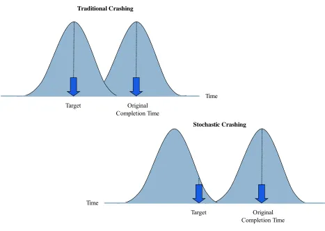
Original Completion Time Target

Time

Original Completion Time Target

Time

Traditional Crashing

[image:20.612.72.539.193.525.2]

Stochastic Crashing

Figure 3.1: Traditional Crashing vs. Stochastic Crashing.

As a way to overcome the limitations of the CPM crashing method, several

simulation-based crashing methods that address the time-cost tradeoff problem have been developed (Bissiri

and Dunbar, 1999; Gutjahr et al., 2000; Haga, 1998; Haga and Marold, 2004; Haga and Marold,

2005), but in general the literature about this topic is limited (Herroelen and Leus, 2005). The

(21)

project cost (lateness penalty plus crashing cost). The next paragraphs summarize some of these

methods.

Bissiri and Dunbar (1999) present a method to crash a project network, which suggest the

use of simulation to obtain the average time of each activity, the critical path, and the near

critical paths. A near critical path in this model is a path which length is smaller than the original

completion date but it is larger than the target completion date after crashing. After the path

information is collected a linear program is applied to determine the optimum crashing strategy.

This method works in a very similar way to the traditional CPM crashing method because it

considers average activity times and looks for a solution in a deterministic manner.

Gutjahr et al. (2000) introduces a stochastic branch-and-bound crashing method, which

objective is to select the set of measures that will reduce the duration of the project, avoiding or

reducing penalty costs, in the most cost-efficient way. Specifically, it is assumed that there is a

group of measures that can be implemented, and each measure may reduce the duration of one or

more activities in the project by a given amount. Each measure is associated with a binary

variable which indicates if the measure is chosen or not.

Haga (1998) along with Haga and Marold (2004), and Haga and Marold (2005) present a

series of papers involving heuristic crashing methods for project management utilizing

simulation.

Haga and Marold (2004), proposed a simulation-based method that deals with the

time-cost trade-off involved with crashing a project. The authors state that “the complete distribution

of project completion time needs to be considered when crashing”. The method that they

proposed is a two steps approach. The first step is to apply the traditional PERT method to crash

(22)

its limit to determine if crashing that activity further reduces the average total cost of the project.

In this research, the authors considered two sources that can increase the cost of the project,

which are crashing costs and overrun costs. The approach that Haga and Marold (2004) followed

tries to optimize the cost of the project, thus if the penalty for late completion is smaller than the

crashing cost of the activities this method may suggest to allow the project to be completed late.

One improvement opportunity identified in this research is that the method presented does not

provide a way to monitor the crashing recommendations that it proposes, which can result in

unnecessary crashing of activities. The approach presented in Haga and Marold (2004) is a

heuristic that doesn’t consider interactions between different activities; essentially it conducts a

one-at-a-time evaluation of the crashing potential of the activities to determine which activities

should be crashed.

As a continuation of the Haga and Marold (2004) research, Haga and Marold (2005)

developed a simulation-based method to monitor and control a project. The output of this method

is a list of dates at which the project manager “should review the project to decide if activities

need to be crashed”. These dates are called crashing points, and they are determined by a

backward run through the project network. Although the concept explained in this research is

very useful, the proposed method requires a large amount of simulation time to evaluate a large

project network and “if the network does not have a single dominant critical path, the algorithm

will likely tend to overly crash the project” (Haga and Marold, 2005). In addition, before the

project starts, this method determines which activities might be crashed.

The methods discussed in this section provide a foundation for solving the time-cost

(23)

3.3 Discrete Optimization via Simulation

When dealing with the stochastic time-cost tradeoff problem, the project managers are

interested in identifying the optimal crashing configuration that minimizes the project cost. Since

the simulation-based crashing methods currently described in the literature are heuristic, there is

an opportunity to develop a method capable of providing an optimal solution to the stochastic

time-cost tradeoff problem.

In the context of simulation, discrete optimization is designed to “maximize or minimize

the expected value of a simulation output random variable whose distribution depends on a finite

vector of controllable decision variables” (Xu et al., 2007). In the case of the stochastic time-cost

tradeoff problem the objective is to minimize the expected value of the project cost which

depends on a vector of integer variables that represent the crashing amount of each activity

Various solution methods for discrete optimization via simulation are presented in the

literature, “including globally convergent random search (GCRS) algorithms, locally convergent

random search (LCRS) algorithms, ranking and selection (R&S), and ordinal optimization (OO)”

(Xu et al., 2007). For additional details please refer to Xu et al. (2007).

One of the most recent algorithms for discrete optimization via simulation is Industrial

Strength COMPASS (ISC). ISC is “a particular implementation of a general framework for

optimizing the expected value of a performance measure of a stochastic simulation with respect

to integer-ordered decision variables” (Xu et al., 2007). ISC is derived from the Convergent

Optimization via Most Promising Area Stochastic Search (COMPASS) framework developed by

Hong and Nelson (2006) for locally convergent, discrete optimization-via-simulation (DOvS).

As indicated by Xu et al. (2007), ISC provides convergence guarantees and statistical inference.

(24)

realistic problems in a reasonable amount of time; however, they lack the convergence

guarantees and statistical inference that ISC provides.

ISC is an initial effort to close the gap that commercial OvS software have in terms of

convergence guarantees, thus it has limitations (Xu et al., 2007):

• Problems with multiple objectives are not supported;

• Only integer-ordered decision variables are considered;

• Only linear-integer inequality constraints are considered; and

• Recommended for problems with up to 10 decision variables.

Although these limitations exist, ISC can be applied to a large segment of discrete simulation

optimization problems.

The optimization procedure implemented by ISC is divided in three phases:

• Global Phase: explores the entire solution space, and identifies sub-regions with potential

good solutions;

• Local Phase: evaluates each sub-region and converges to local optimal solutions; and

• Clean Up Phase: selects the best solution among the local optima identified in the Local

Phase, and estimates its value with the precision specified by the user.

Since the stochastic time-cost tradeoff problem is a problem suitable for DOvS, ISC is a

good candidate for an optimization engine.

3.4 Discussion

While reviewing literature relevant to the time-cost trade-off problem in project

management, certain opportunities for improvement have been identified. One opportunity is

(25)

nature and provide a solution to the problem, but do not guarantee optimality. To address this

opportunity a simulation-based crashing method (presented in Chapter 4) is developed in which a

simulation model interacts with an optimization engine to obtain an optimal solution. Another

opportunity is that the simulation-based methods that are presented in Section 3.2 are designed to

solve only a portion of the problems that project managers may face. To expand the current

literature a method is developed (and presented in Chapter 5) to solve a generalized version of

the stochastic time-cost tradeoff problem, which relaxes the assumptions considered by the

traditionally defined time-cost tradeoff problem.

From the methods presented in Section 3.2, the methods that are more closely related (in

terms of the solution the method provides) to the methods presented in this thesis are Haga and

Marold (2004, 2005). Table 3.1 summarizes these methods and the ones presented in this thesis.

Regarding the traditionally defined time-cost tradeoff problem, in the case of a single

critical path the method of Haga and Marold (2004) provides an optimal solution in the static

phase, which is prior to the start of the project. For the dynamic phase (throughout the project

execution) Haga and Marold (2005) provides a heuristic solution; essentially the method

provides, prior to the start of the project, a set of completion times (crashing points) for the

activities by which the activities should be completed, and then, during the project, the project

manager needs to decide if the activities will be completed by those points; if the project

manager decides that the activities won’t be completed by the crashing points, the activities

should be crashed. For the case of multiple potential critical paths Haga and Marold (2004)

provide a heuristic solution for the static phase. The dynamic solution (Haga and Marold 2005) is

(26)

The first method developed and presented in this thesis (OTCM), which is focused on the

traditionally defined time-cost tradeoff problem, provides (for the static evaluation) an optimal

solution for the cases of single or multiple critical paths. For the dynamic phase OTCM is a

heuristic solution because the user specifies the times for the dynamic reevaluations. If the

project is continuously reevaluated the solution would be optimal.

Table 3.1. Summary of Different Approaches to the Time-Cost Tradeoff Problem (CP ≡ Critical Path).

Static Method (Haga & Marold, 2004) Dynamic Method (Haga & Marold, 2005)

Static Method Dynamic Method

Single CP; Integer

Crashing; Linear Costs Optimal Heuristic (OTCM) Optimal

Heuristic (OTCM) Multiple CP; Integer

Crashing; Linear Costs Heuristic Heuristic (OTCM) Optimal

Heuristic (OTCM) Single/Multiple CP;

Varying Mean of Base Alternative; Non-linear, ordered Costs

- - Heuristic

(DSA)

Heuristic (DSA)

Single/Multiple CP; Varying Distribution of Base Alternative; Non-linear, not ordered Costs

- - Heuristic _(DSA) Heuristic _(DSA)

In addition, a method that more accurately represent the situations that the project

manager might encounter has been developed. The method (DSA) relaxes the assumptions

traditionally associated with the alternatives associated to each activity. DSA is a heuristic

because the optimization engine used is not designed to guarantee optimality for these cases. If

(27)

4. OPTIMAL CRASHING METHODS FOR TRADITIONALLY DEFINED

PROJECT MANAGEMENT PROBLEMS

Although the intention of this research is to solve the generalized time-cost tradeoff

problem, the initial methods that are developed and presented are for the traditionally defined

application of crashing methods to project management. Given that much of the current literature

(e.g. Bissiri and Dunbar, 1999; Gutjahr et al., 2000; Haga and Marold, 2004) focuses on the

traditional definition of crashing and assuming that this definition adequately describes a portion

of the projects to which project management techniques are applied, optimal crashing methods

for this traditionally defined scenario are presented in this chapter. The methods developed for

the generalized time-cost tradeoff problem are presented in Chapter 5.

Project management problems involving crashing are traditionally defined as follows.

Given a project defined by individual activities, their precedence relationships, and stochastic

activity durations, a project network can be developed. An example of such a project (Sample

Project) having 11 activities is described in Table 4.1; Figure 4.1 illustrates the project network

where the nodes represent the activities and the arcs (edges) represent the precedence

relationships. In this type of project, crashing is defined as “spend[ing] more money on the

project in order to speed up accomplishment of scheduled activities” (Rosenau and Githens,

2005). The crashing potential of an activity is the maximum number of time units by which an

activity’s time can be reduced. In this traditional definition, activities are typically crashed in

integer time units up to the crashing potential, and the associated crashing cost is assumed to be

linear (that is, each time unit by which the activity is crashed has the same cost). For each

activity in the example, the maximum crashing potential is specified in Table 4.1 along with the

(28)

a linear function of the quantity of time by which the project is late. For example, a project that is

due at time 70 with a lateness penalty of 40 per time unit would have the following penalty

function, ⎩ ⎨ ⎧ > − ≤ = 70 τ if ), 70 τ ( 40 70 τ if , 0 ) τ , (T PF .

The objective of the traditionally defined problem is to determine the activities to crash

in order to minimize the average project total cost, where the total cost is defined as crashing cost

plus any penalty due to lateness.

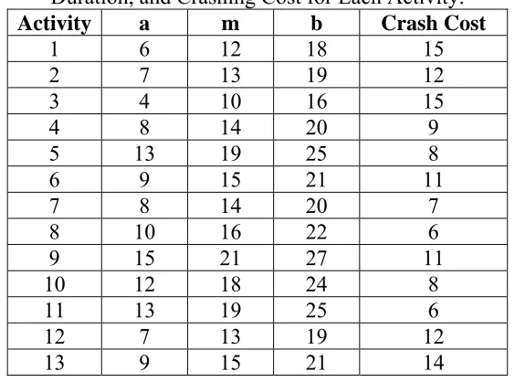
Table 4.1: Sample Project Specifications.

Activity Duration Crashing Unit Crashing Activity Predecessors Minimum Mode Maximum Potential Cost

1 - 8 10 12 3 6

2 1 6 10 14 3 3

3 1 6 8 10 3 5

4 3 10 15 20 3 4

5 2 12 17 22 3 5

6 2,4 3 5 7 3 8

7 5 6 9 12 3 5

8 6 4 6 8 3 5

9 4 11 13 15 3 2

10 7,8,9 13 15 17 3 8

11 10 5 7 9 3 7

(29)

The purpose of this first stage of the research is to develop static and dynamic

simulation-based analysis methods for the traditionally defined time-cost tradeoff problem that are capable

of evaluating project networks to answer the following questions:

• Which activities should be crashed in order to minimize the average project cost?

• To what extent should the activities be crashed?

• Should the crashing configuration be changed throughout the project?

The method presented in this section is named the Optimal Traditional Crashing Method

(OTCM). The overall OTCM procedure is presented in two phases. Phase I considers the

evaluation of the project prior to the start of the project. This phase will produce an optimal

crashing strategy with respect to information available prior to the start of the project. During

Phase II, which is applied as the project progresses, dynamic reevaluations of the project are

performed in order to consider the known durations (and sunk costs) of completed activities and

the effect of the uncertainty of the durations of the remaining activities, and to determine the

optimal crashing strategy from that point forward.

In the next sections, Phase I and Phase II of the OTCM procedure are presented.

Although the two phases are designed to be used together to maximize the benefit of the method,

Phase I can be applied independently from Phase II at the start of the project with Phase II being

(30)

4.1 Assumptions Considered in the OTCM Method

The OTCM method is designed taking the following assumptions into account:

1) Crashing an activity is defined as reducing the activity time by an integer number of time

units, thereby shifting the location of the distribution and maintaining the shape

(variance, skewness, etc.) of the activity time distribution;

2) Activity times are independent;

3) Activity time distributions can be estimated, using a probability distribution that will not

result in negative activity times when crashing is applied. Using the beta distribution or

the triangular distribution to represent activity times is common in the field of project

management (Lee and Arditi, 2006; Lu and AbouRizk, 2000; Haga and Marold, 2004)

and this convention is kept for the OTCM examples and experiments. The probability

distribution of each activity, in this case, is defined by three estimates consisting of the

optimistic (minimum), most likely, and pessimistic (maximum) duration times;

4) Crashing costs are known or can be estimated very accurately;

5) Penalty costs for late completion, represented by a linear function, are defined before the

start the project; and

6) Precedence constraints are assumed to be strictly defined (a successor activity cannot

begin until all the predecessors have been completed).

4.2 OTCM Phase I: Optimal Crashing Method Applied Prior to the Start of the Project The objective of Phase I of the method is to obtain the optimal crashing configuration

prior to the start of the project that will minimize the expected total project cost with respect to

(31)

the uncertainty associated with the duration of each activity is considered, which is represented

by probability distributions.

Phase I involves the following procedure:

• Defining the project in terms of the activities, predecessors, activity times, crashing

potential of each activity in the network and the related costs, and the penalty cost

function;

• Constructing a simulation model of the project network;

• Utilizing a stochastic simulation optimization tool such as Industrial Strength COMPASS

(ISC) to determine the optimal project crashing configuration;

• Evaluating the effect of not crashing the project (original crashing configuration) and the

effect of implementing the optimal crashing configuration with the OTCM project

simulator;

• Implementing the optimal crashing solution; and

• Proceeding to Phase II (optional).

The first step of the process is to specify the parameters that define the project network

and the optimization problem. The parameters include the number of activities, the probability

distribution associated with the completion time of each activity, the predecessors of each

activity, the maximum completion time by which no penalties are applied, the maximum amount

by which an activity can be crashed (crashing potential), and the cost of crashing each activity.

Note that the crashing potential of activities determines the solution space and complexity of

optimization the problem (e.g. if there are 15 activities in a project and each one could be crash

by 0, 1, or 2 units, thus each having a crashing potential of 2, the number of possible crashing

(32)

A simulation model of the project network is constructed after the input parameters are

provided. The simulation model represents all the activities in the project and the precedence

relationships that exist among them. The model is used to evaluate the various crashing

configurations that could be implemented in the project. Evaluating a crashing configuration

involves running a specified number of replications (instances) of the project network, under the

crashing configuration that is being considered, in order to estimate the average project cost

resulting from that configuration. Running a replication of the simulation model representing the

project network involves sampling an activity time from the probability distribution representing

the duration of each activity, reducing the sampled duration according to the crashing

configuration that is being considered, calculating the start time and completion time of each

activity taking into account that precedence relationships must be enforced, calculating the

completion time of the project, calculating the penalty for late completion (if any), and finally

computing the project cost, which consists of the lateness penalty and the crashing cost.

Once the simulation model has been designed, and the crashing potential for each activity

on the network has been identified, it is possible to run the optimization (OTCM program). The

simulation-based optimization engine for the OTCM method is designed to optimize the

performance measure generated by the simulation model, given that the performance measure

depends on integer decision variables. The optimization engine also provides convergence

guarantees within a precision level specified by the user. The stochastic optimization is

responsible for minimizing the average cost subject to constraints that indicate that the crashing

amount of each activity cannot be greater than its crashing potential. The engine searches the

solution space for potential optimal solutions. Once a potential solution (crashing configuration)

(33)

specified number of instances of the project for the crashing configuration sent by the

optimization engine and calculates the cost of the project in each instance; the number of

instances to be evaluated is determined by the optimization engine. The cost of each evaluated

instance of the project is sent to the stochastic optimization engine which tests the configuration

for optimality. The optimization engine continues the evaluation of potential solutions until the

optimal solution has been identified. At that point, the optimal solution is reported, which

includes the crashing configuration that minimizes the average project cost and statistics

associated with the optimal solution (sample mean of project cost, sample variance of project

cost, and a 95% confidence interval on project cost).

After obtaining the optimal solution, the OTCM project simulator is used to evaluate the

impact that implementing the original or the optimal crashing configuration has on the project

cost. The output of the project simulator includes statistics about the project completion time and

project cost (sample mean, sample variance, and a 95% confidence interval), and provides the

data required to plot the distributions of project completion time and project cost under both

crashing configurations (original vs. optimal). Using these pieces of information, the project

manager can decide if the optimal crashing configuration will be implemented. The project

manager also decides if Phase II will be applied.

4.3 OTCM Phase I Example

To illustrate Phase I of the OTCM method, the Sample Project discussed in Section 4 is

used. The details are shown again here for convenience in Table 4.2 and Figure 4.2. In this

example, the project network consisting of 11 activities has multiple potential critical paths and

(34)

activity in this project has a crashing potential of up to 3 time units. The respective estimates of

the minimum, most likely, and maximum activity times used to fit a beta distribution to the

activity durations, and the crashing costs per unit are shown in Table 4.2. The target completion

time of the project is time 70, and the equation defining the penalty cost for late completion is

⎩ ⎨ ⎧ > − ≤ = 70 τ if ), 70 τ ( 40 70 τ if , 0 ) τ , (T PF

where τ is the resulting completion time of the project. Figure 4.3 depicts the input file used in this example (see Section 4.6.1 for a detailed discussion of input file parameters).

Table 4.2: OTCM Phase I Example - Project Specifications.

Activity Duration Crashing Unit Crashing Activity Predecessors Minimum Mode Maximum Potential Cost

1 - 8 10 12 3 6

2 1 6 10 14 3 3

3 1 6 8 10 3 5

4 3 10 15 20 3 4

5 2 12 17 22 3 5

6 2,4 3 5 7 3 8

7 5 6 9 12 3 5

8 6 4 6 8 3 5

9 4 11 13 15 3 2

10 7,8,9 13 15 17 3 8

11 10 5 7 9 3 7

(35)

n 11

T 70

P 40 SC 0

NPi 0 1 1 1 1 2 1 1 1 3 1

0 1 1 3 2

2 4 5 6 4

7 8 9 10

CPi 3 3 3 3 3 3 3 3 3 3 3 B8 10 12

B6 10 14 B6 8 10 B10 15 20 Activity B12 17 22 Duration B3 5 7 Distribution B6 9 12 (Ai) B4 6 8

B11 13 15 B13 15 17 B5 7 9 6 3 5 4 5 Crash Costs 8 (CCi) 5 5 2 8 7 ISC output

Parameters 999999 1 0 -1 -1 0 -1 1 -1 -1 -1 0.01 1 0.01 0.5 50 10 0 50

Figure 4.3: OTCM Phase I Example - Input File. Predecessors

(PMij = 1 for each j in row i,

(36)

The OTCM program was used to obtain the optimal crashing configuration which is to

crash activity 2 two time units, and activity 9 one time unit, with an estimated average project

cost of 14.55 and an associated project cost variance of 435.56 (the OTCM program ran 22,686

replications to compute these estimates). The 95% confidence interval on the average project

cost when the solution provided by Phase I is implemented is:

[14.28 ≤ µ₀≤_14.82].

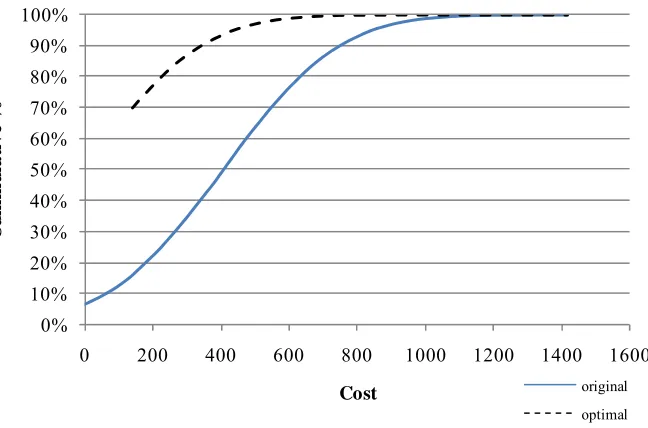
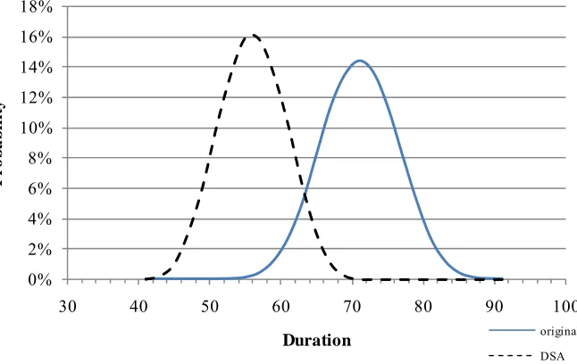
The original project without crashing and the project with the optimal crashing configuration are

each simulated 50,000 times with the OTCM project simulator to produce the distribution of

completion time (Figure 4.4) and the cumulative distribution of the total project cost (Figure

4.5). In addition, Table 4.3 provides the average and standard deviation of the project duration

and project cost.

0% 2% 4% 6% 8% 10% 12% 14% 16% 18% 20%

58 60 62 64 66 68 70 72 74 76 78

P

r

ob

ab

il

it

y

Duration original

optimal

(37)

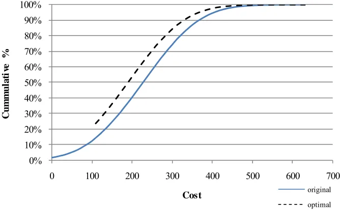
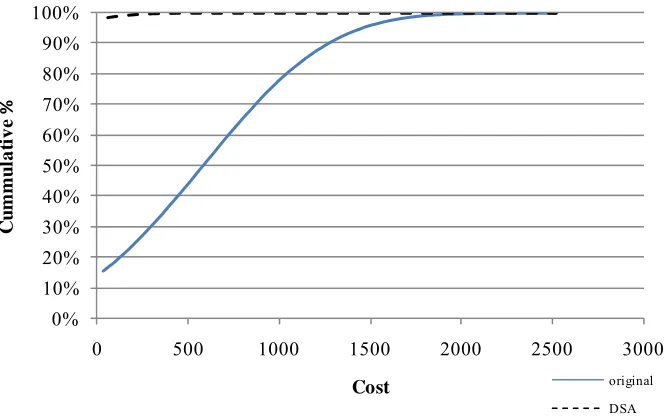
0% 10% 20% 30% 40% 50% 60% 70% 80% 90% 100%

0 50 100 150 200 250 300 350

Cu

m

u

la

ti

v

e

%

Cost original

optimal

Figure 4.5: OTCM Phase I Example - Original versus Optimal Project Cost.

Table 4.3: OTCM Phase I Example - Summarized Comparison between No Crashing and Optimal Crashing.

Duration Cost

Average Std. Dev. Average Std. Dev. Original 69.22 2.11 20.41 38.73 Optimal 67.85 2.06 14.35 20.43

To provide statistical evidence about the cost reduction produced by the Phase I method

over no crashing, using paired data a 95% confidence interval is built on the difference between

the average cost of the project when no crashing is applied and the project when the solution

provided by Phase I is implemented:

[5.85 ≤ µ₀₁_,₅₀₀₀₀ ≤ 6.28].

These results indicates that there is a significant difference between the average cost of no

crashing versus the average cost of implementing the Phase I solution, and indicates that when

(38)

4.4 OTCM Phase II: Dynamic Crashing

In Phase I, prior to the start of the project, an initial optimal crashing configuration is

obtained by analyzing the entire project network. This initial optimal crashing configuration

considers the uncertainty associated with the duration of all the activities of the project. As

activities are completed, the uncertainty associated with their duration is eliminated. Thus the

overall uncertainty about the project completion time is reduced; as a result the initial optimal

solution might change. The purpose of the Phase II (dynamic) method is to determine the optimal

crashing configuration for the remaining activities.

In addition to the general assumptions of the OTCM method, the following assumptions

are applied to Phase II:

• The reevaluations points occur just prior to starting an activity that has been

recommended for crashing previously. The initial reevaluation points are assumed as the

crashing points identified in Phase I;

• The resources required to crash an activity are available at the moment of making a

crashing decision, i.e. the lead time to acquire or change the resources is 0; and

• The remaining time for activities in progress is known or can be estimated very

accurately.

Due to the first assumption, Phase II is a heuristic. In order for Phase II to be optimal

throughout the project, the project network should be constantly evaluated. Constantly evaluating

the project is not practical and cost prohibitive, thus, in this research it has been assumed that the

project is reevaluated when the start time of an activity identified to be crashed is encountered

(the intention of the reevaluations in this case is to verify if the activity still needs to be crashed

(39)

the activity doesn’t need to be crashed or needs to be crashed by a smaller amount). In addition,

the first assumption indicates that if no activities should be crashed, according to the solution

provided by Phase I, there is no need to implement Phase II. However, although not tested here

the project manager could decide implementing Phase II at any time after the start of the project,

in order to determine if crashing would make economic sense due to the duration of activities

previously completed, or as changes are made to the project plan.

The OTCM Phase II procedure involves:

1. Updating the project information to reflect the current status of the project;

2. Updating the simulation model of the project network;

3. Reevaluating the remaining project network using the OTCM program (as described in

Phase I) when an activity that requires crashing is encountered;

4. Evaluating the effects of implementing the previous crashing configuration and the new

optimal crashing configuration with the OTCM project simulator;

5. Implementing the project network under the new crashing configuration and continuing

until either:

a) the next activity that requires crashing is encountered and go to step 1; or

b) the project is complete.

Note that for each iteration of steps 1-4 of the dynamic crashing procedure, a new

crashing configuration for the remainder of the project will be identified that takes into account

the sunk activity times and costs associated with the activities in progress and the activities that

have been completed.

The first step in the procedure that Phase II follows is to update the information that

(40)

potential is set to 0 and their duration is represented by their actual (in the case of completed

activities) or estimated (in the case of activities in process) duration (instead of by a probability

distribution). For the activities that haven’t started the crashing potential, the crashing cost, and

the probability distribution of completion time are considered to be equal to the values used in

Phase I. Also, Phase II considers the same target completion time and the same penalty function

used in Phase I (note that since the project information is updated before each reevaluation it is

possible to include information different than the one provided in Phase I or in previous Phase II

reevaluations). The updated information is input into the simulation model to guarantee that the

simulation model is an accurate representation of the project network.

After the simulation model is updated the optimization process, as described in Phase I, is

applied. Then, the optimal crashing configuration provided by the OTCM program and the

previous crashing configuration are evaluated with the OTCM project simulator. As in Phase I,

the project manager uses the output of the OTCM project simulator to decide whether or not to

implement the solution provided by the Phase II reevaluation. This process continues until

another reevaluation point is encountered or until the project is complete.

4.5 OTCM Phase II Example

The Sample Project used to illustrate Phase I is now used to demonstrate Phase II of the

OTCM method. Recall, that the Sample Project consisted of 11 activities with the project details

outlined in Table 4.2 and the corresponding project network shown in Figure 4.2. The optimal

crashing configuration obtained when Phase I of the OTCM was applied to the Sample Project

specified that activity 2 should be crashed two time units and activity 9 should be crashed one

(41)

if any of the activities that start at the project starting time are recommended by Phase I to be

crashed, the crashing should be applied.) To facilitate a direct comparison among project

implementations with no crashing applied, using the result of OTCM Phase I only, and the full

implementation of the OTCM method (Phases I and II), one instance of the Sample Project is

simulated. The resulting activity times without any crashing applied are shown in Table 4.4.

After the project begins, the OTCM Phase II procedure specifies that the project

reevaluation points (the points at which the crashing configuration is reevaluated) will occur just

prior to starting activities that have previously been identified by the OTCM method to be

crashed. In the Sample Project, at time 10.88 which corresponds to the completion time of

activity 1, the first activity that Phase I specified to crash is encountered. Consequently, the time

just prior to the start of activity 2 will serve as the reevaluation point. Figure 4.6 depicts the

status of the project up to the first reevaluation point.

Table 4.4: OTCM Phase II Example - Sample Project Instance. Activity Duration

1 10.88 2 7.32 3 8.15 4 17.91 5 15.75 6 4.87 7 7.95 8 4.86 9 13.35 10 15.82 11 6.54

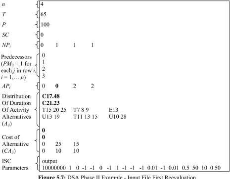
To implement the reevaluation, the OCTM program is invoked with an input file that

reflects the current project status. This input file is shown in Figure 4.7. The bold entries indicate

(42)

Project, the crashing potential for each of the remaining activities remains the same throughout

the project. However, any changes to the project parameters including the activity durations and

crashing potential can be updated at any time and included in the reevaluation.) Thus, the

updates to the input file needed for this reevaluation include changing the crashing potential of

activity 1 to 0 and entering the actual duration of activity 1 as a constant time of 10.88 (indicated

as C10.88 in the input file, where C denotes a constant).

Legend:

Completed & Not Crashed

In process & Not Crashed

Completed & Crashed

In process & Crashed

Not Started

Evaluation Point 2

3

4

7

6 5

8

9

10 11

1

Figure 4.6: OTCM Phase II Example - Network Status by First Reevaluation Point.

Upon running the OTCM program, a new crashing configuration is obtained for the

remaining activities. Table 4.5 shows the resulting crashing configuration which specifies that

activity 2 is to be crashed two time units (this in consistent with the result of Phase I), and since

the project is lagging due to a longer than expected duration of activity 1, the crashing

configuration also specifies crashing activity 9 by two time units (rather than 1 time unit as

specified by Phase 1). Table 4.6 indicates the new estimate of the average project cost (Sample

(43)

which are 19.06 and 601.48, respectively. In addition, the number of simulated instances of the

project used to obtain the estimates, 30,856 replications, is also listed.

n 11

T 70

P 40

SC 0

NPi 0 1 1 1 1 2 1 1 1 3 1

0 1 1 3 2

2 4 5 6 4

7 8 9 10

CPi 0 3 3 3 3 3 3 3 3 3 3 C10.88

B6 10 14 B6 8 10 B10 15 20 Activity B12 17 22 Duration B3 5 7 Distribution B6 9 12 (Ai) B4 6 8

B11 13 15 B13 15 17 B5 7 9 6 3 5 4 5 Crash Costs 8 (CCi) 5 5 2 8 7 ISC output

Parameters 999999 1 0 -1 -1 0 -1 1 -1 -1 -1 0.01 1 0.01 0.5 50 10 0 50

Figure 4.7: OTCM Phase II Example - Input File First Reevaluation. Predecessors

(PMij = 1 for each j in row i,

(44)

Table 4.5: OTCM Phase II Example - Crashing Configuration Provided by First Reevaluation.

Activity

1 2 3 4 5 6 7 8 9 10 11 Crash

Amount 0

2

0 0 0 0 0 0

2

0 0

Table 4.6: OTCM Phase II Example - Summary of Solution Provided by First Reevaluation. Replications 30,856

Sample Mean of Cost 19.06 Sample Variance of Cost 601.48

Upon implementing the specified crashing amount of 2 time units for activity 2, the

project proceeds until the next reevaluation point in encountered. This occurs just prior to the

start of activity 9 which is realized at time 36.94. By that time activities 1 through 5 have been

completed, activity 7 is in progress, and the remaining activities haven’t started. Figure 4.8

shows the status of the project up to the second reevaluation point. The input file of the OTCM

program is updated once again to reflect the current project status. The update includes setting

the crashing potential of activities 1 through 5 to 0 and replacing the probability distribution that

previously represented their duration by their actual duration; since activity 7 is in progress its

crashing potential is also set to 0 and its duration (assumed to be accurately estimated) is

considered to be a constant time of 7.95. In addition, the input file is updated to include the sunk

cost of crashing activity 2; since activity 2 was crashed twice and the crashing cost per time unit

of activity 2 is equal to 3, the sunk cost is equal to 6. After updating the input file the OTCM

program is executed, and a new crashing configuration is obtained. Table 4.7 shows the new

crashing configuration which indicates that activity 9 is to be crashed three time units (even more

than previously indicated by the first reevaluation), and since the project continues to run behind

(45)

Table 4.8 shows the new estimates for the average project cost and the project cost variance

which are 24.84 and 23.19, respectively (545 instances of the project were simulated to obtain

these estimates).

Legend:

Completed & Not Crashed

In process & Not Crashed

Completed & Crashed

In process & Crashed

Not Started

Evaluation Point

6 8

9

10 11

1

5

3

4

7 2

Figure 4.8: OTCM Phase II Example - Network Status by Second Reevaluation Point. Table 4.7: OTCM Phase II Example - Crashing Configuration Provided by Second

Reevaluation.

Activity

1 2 3 4 5 6 7 8 9 10 11 Crash

Amount 0

2

0 0 0 0 0

1 3

0

1

Table 4.8: OTCM Phase II Example - Summary of Solution Provided by Second Reevaluation. Replications 545

Sample Mean of Cost 24.84 Sample Variance of Cost 23.19

Activity 9 is crashed three time units as indicated by the crashing configuration, and the

project continues. The new reevaluation point is encountered at time 41.81, which corresponds to

(46)

9 is in progress, therefore the input file required for the next reevaluation is updated to indicate

that the crashing potential of these activities is equal to 0 and that their durations are represented

by a constant time. The crash cost of activity 9 is 2 per time unit, and since it was crashed three

times the cost of crashing activity 9 is 6; this cost is added

Project management: a simulation-based optimization method for dynamic time-cost tradeoff decisions

Rochester Institute of Technology

RIT Scholar Works

Rochester Institute of Technology

PROJECT MANAGEMENT: A SIMULATION-BASED OPTIMIZATION METHOD FOR DYNAMIC TIME-COST TRADEOFF DECISIONS

A Thesis

ROCHESTER, NEW YORK

ABSTRACT

TABLE OF CONTENTS

5. DYNAMIC SELECTION OF ACTIVITY ALTERNATIVES ...84

6. MS PROJECT INTERFACE ...133

7. CONCLUSIONS & RECOMMENDATIONS FOR FUTURE RESEARCH ...149

REFERENCES ...152

2. PROBLEM STATEMENT

3. LITERATURE REVIEW

3.1 Project Management: Project Scheduling

3.2 Project Management: Time-Cost Tradeoffs

Traditional Crashing

3.3 Discrete Optimization via Simulation

3.4 Discussion

Static Method (Haga & Marold, 2004) Dynamic Method (Haga & Marold, 2005)

4. OPTIMAL CRASHING METHODS FOR TRADITIONALLY DEFINED

Activity Duration Crashing Unit Crashing Activity Predecessors Minimum Mode Maximum Potential Cost

4.1 Assumptions Considered in the OTCM Method

4.3 OTCM Phase I Example

Activity Duration Crashing Unit Crashing Activity Predecessors Minimum Mode Maximum Potential Cost

Duration Cost

4.4 OTCM Phase II: Dynamic Crashing

4.5 OTCM Phase II Example